Wavestar prototype at Roshage Performance data for ForskVE project no phase 1 & 2, January 2013

(1)

Wavestar

prototype

at

Roshage

Performance

data

for

ForskVE

project

no

2009

‐

1

‐

10305

phase

1

&

2,

January

2013

Wave Star A/S

Park Allé 350A

2605 Brøndby

Denmark

Tel: +45 4040 4696

(2)

Table

of

contents

1 Summary ... 3

2 History of events and performance ... 6

3 Production data in phase 1 ... 10

4 Production data in phase 2 ... 11

5 Future plans and activities ... 14

6 References ... 15

Appendix A Wave climate at the location ... 16

Appendix B Production estimates by the WEC model ... 20

(3)

1

Summary

A contract between Wave Star A/S and EnergiNet.dk was established in July 2010 with the project title “En‐ ergy production on Roshage test systems (WSE‐02)”, project no. 2009‐1‐10305. The aim of the project was

to document that the Wavestar wave energy converter at Roshage was able to deliver the expected power

according to the actual wave climate. The project is part of the so‐called ForskVE‐programme [1], and it is

completed with Aalborg University as partner. Since 1 May 2010 Wave Star A/S has been measuring the

waves at the location and the power produced by the Wavestar prototype. Every month a report and ac‐

companying data file containing the raw measurements are submitted to EnergiNet.dk for approval [2].

Waves and power production are measured directly on‐board the Wavestar prototype. An ultrasonic wave

sensor is providing wave recordings at the exact location of the device. Figure 1 in the next page is showing

the different power conversion stages. Two definitions are important in the report.

Hydraulic power, Ph [W]: The hydraulic power is measured at the hydraulic actuator, calculated by multiply‐

ing of the pressure across the cylinder and the flow in the cylinder. The hydraulic power of the prototype is

the sum of the hydraulic power of both floats, Ph = Ph1 + Ph2. The hydraulic energy, referred to as Eh, is the integration of the instantaneous hydraulic power over time.

Electrical power, Pe [W]: The electrical and consequently generated power is measured at the output of the generator, calculated by multiplying the voltage and the current. The electrical power of the prototype is

the sum of the electric power of both floats, Pe = Pe1 + Pe2. The electrical energy, referred to as Ee, is the integration of the instantaneous electrical power over time.

The project was split in two phases:

 Phase 1, May 2010 to September 2011: Focus was to demonstrate that the hydraulic power was

higher than a specified target power performance curve. Phase 1 was finished in September 2011

where 14754 valid ten minute records with power production higher than the specifications, were

recorded, documented and approved by EnergiNet.dk.

 Phase 2, October 2012 to December 2012 (three months): Emphasis was on the electrical energy.

In phase 2 the capability of the machine to deliver at least 14.0[electrical MWh] in a three month

period was documented. Phase 2 was completed after phase 1 was completed when the machine

was ready for automatic continuous unmanned operation.

This document is the final report which presents the power measurements from both phase 1 and phase 2.

Table 1 and 2 summarizes the measured results. The total electrical energy produced by the two generators

was 52.9[MWh] in the period from May 2010 to December 2012. However, the largest amount of energy

per month was produced during the three months in phase 2 where 15.6[MWh] was delivered by the gen‐

erators. In phase 1 the absorbed hydraulic energy was high but the produced electricity and the operational

time was low. However, in phase 2 the operational time and the PTO efficiency was high resulting in a high

electrical energy production. Details on measurements of the power production during phase 1 are given in

Section 3, and phase 2 results are given in Section 4.

Period Hydraulic energy [MWh] Electrical energy [MWh] PTO efficiency [%]

May‐10 to Sep‐11 (phase 1) 51.6 6.9 13.3

Oct‐11 to Sep‐12 52.8 30.4 57.6

Oct‐12 to Dec‐12 (phase 2) 26.0 15.6 60.1

May‐10 to Dec‐12 130.4 52.9 ‐

(4)

Period Operational time (%) Production (%)

May‐10 to Sep‐11 (phase 1) 47.8 63.6

Oct‐11 to Sep‐12 66.7 64.3

Oct‐12 to Dec‐12 (phase 2) 99.4 82.3

May‐10 to Dec‐12 59.7 65.8

Table 2: Summary of the measured energy production in the whole period covering phase 1 and phase 2.

The target in phase 2 was to produce at least 14.0[electrical MWh] in the three month period. During the

three month period from October 2012 to December 2012 the Wavestar demonstrator produced

15.6[MWh], which more than fulfills the expectations for the power performance. The target production

was calculated using historic wave data measured by a wave rider in deep water offshore Hanstholm. How‐

ever, as described in Appendix A, the actual measured waves in the shallow water at the Wavestar location

are considerably smaller. Nevertheless, the goal was exceeded significantly. The reason was that the opera‐

tional and production time was exceeding the expectations. The average operational time during phase 2

was 99.4[%] and the converter produced electricity to the grid in 82.3[%] of this time, see Table 2.

Figure 1: Overview of energy conversion stages of Wavestar’s prototype in Hanstholm. The hydraulic power Ph[W] is measured at the hydraulic actuator (pressure across the cylinder multiplied by the flow in the cylinder). The electrical power Pe[W] is measured at the output of the generator (voltage multiplied by current).

(5)

A numerical model has been developed to make power and energy estimations of the Wavestar converter

depending on physical configuration (e.g. number of floats) and wave climate at a specific location. The

model results are described in detail in Appendix B and the wave climate at the site used for the calcula‐

tions is described in Appendix A. The results show an expected production by the Roshage machine of

46[MWh/year] which corresponds to 46/4 = 11.5[MWh] in a three month period (taking three months as

an average quarter of a year). Estimations for the Roshage WEC using the numerical model are provided in

the right column of Table 3. It is seen that the measured electrical energy of 15.6[MWh] was somewhat

higher than the model estimate. The maximum measured power was 32.4[kW] which was recorded when

the significant wave height was 2.6[m]. The model estimate provided a maximum power of 38[kW], which

is higher than the measured maximum. The measured power performance in high waves shows a large

spread with a general trend lower than the model estimation. In Appendix A it is explained that due to the

low water depth at the location the waves are steep and breaking when the significant wave height is high‐

er than approximately 2.0[m]. Such waves are not ideal for the power performance and the deviation be‐

tween the model estimate and the achieved measured power can be explained by the influence of steep

and breaking waves.

Parameter Measured at Roshage WEC Estimated by WEC model

Total electrical energy produced: Ee[MWh] 15.6 11.5

Max. generated electrical power: max. Pe[kW] 32.4 38

Table 3: Comparison of measured and estimated electrical energy and maximum power in phase 2.

(6)

2

History

of

events

and

performance

In September 2009 Wave Star installed a large‐scale test and demonstration Wave Energy Converter (WEC)

by Roshage pier near Hanstholm at the Western coast of Denmark, see Figure 3 and Figure 4 on the follow‐

ing page. The WEC is a prototype/test section of a complete commercial 600 kW WEC. As shown in Figure 5

and Table 4 the prototype has 2 floats placed on one side whereas the full commercial converter will have

20 floats (10 floats on each side). The prototype was installed at a water depth of approximately 5[m] while

the commercial converter is expected to be installed at water depths of 10 to 20[m]. Several publications

about the prototype and the achieved results have been submitted to scientific conferences and journals,

see e.g.[4,6‐8]. Data concerning the performance of the platform together with the sea state is gathered

continuously. It is valuable knowledge concerning the long term robustness of the platform which may indi‐

cate whether modifications on the future platforms should be considered. The primary purposes of the test

section are outlined below, and the main results received so far concerning the last bullets are given in the

following chapters.

 Test the structure and components  Prove the storm protection strategy

 Provide a test‐platform for future new components  Demonstrate the efficiency of the power take off  Document the ability to be in daily operation 24/7/365

 Check that the measured power absorption is according to the expectations

Furthermore, the WEC is used as a demonstration plant for politicians, journalists, investors and other

stakeholders. The WEC can be accessed at any time and in any weather condition due to its place by the

Roshage pier and a 300 meters long access bridge.

After an initial period of finalizing the installation and testing, the WEC was launched for production in Jan‐

uary 2010 and in May 2010 automatic unmanned operation was initiated. The number of operational hours

per month has increased significantly during the following months, but experience with the initial period of

continuous automatic unmanned operation has shown difficulties in ensuring the ability to be in daily oper‐

ation 24/7/365. The control software has been updated several times with improvement in robustness and

power performance efficiency. The combination of the extension in the operational time and improvement

of power level has increased the kWh’s produced each month. An outline of the events is shown in Figure

2.

(7)

Figure 3: Wavestar prototype. Top: Location of site (Google Earth). Bottom left: Photo of installation by barge. Bottom centre: Photo of storm protection. Bottom Right: Photo of normal operation.

Figure 4: View of Wavestar prototype from the beach. The distance to the prototype from the beach is 300[m].

Gangway Footbridge 4 m above top of pier

(8)

Figure 5: Commercial converter with 20 floats (left) and test‐section at Hanstholm with two floats (right).

Parameter Commercial Wavestar C6‐600 kW Prototype at Hanstholm

Number of floats 20 2

Float diameter Ø6 m Ø5 m

Maximum water depth (extreme) 20 m 8 m

Maximum wave height (operation) 8 m 6 m

Water depth 10 to 20 m 5 to 8 m

Arm length 12 m 10 m

Main structure dimensions 80m x 17m x 6.5m (LxWxH) 32m x 17m x 6.5m

Length of legs Site depended, ~ 15‐25 m above MWL ~ 18 m above MWL

Operation height 6.5 m above MWL 5.5 m above MWL

Storm secure height Site depended, ~ 6‐15 m above MWL ~ 8 m above MWL

Weight 1600 Tons 1000 Tons

Materials Main structure: Steel.

Floats: Fibreglass

Main structure: Steel Floats: Fibreglass

Foundation Four skirted spud cans, or two mono piles or gravi‐

ty based foundations

Four gravity based founda‐ tions

Design service life Minimum 20 years Minimum 20 years

Maintenance interval 1 service period per year ‐

Nominal electrical power 600 kW 110 kW*)

Table 4: Technical Data for Wavestar C6‐Converter and Prototype at Hanstholm. MWL is Mean Water Level. *) Delib‐ erately over‐rated to allow different tests.

When the significant wave height exceeds a certain limit the machine automatically enters storm protec‐

tion mode. Storm protection involves un‐ballasting the floats and retracting the hydraulic cylinders which

thereby pull the floats out of the water. In general there has been no major problem with the design of the

prototype. All structural and mechanical components in the WEC have proven functionality as intended.

The WEC has survived five large storms with no damages and no service afterwards (Storms officially regis‐

tered by the Danish Meteorological Institute on 18/11 2009, 7‐8/2 2011, 27‐28/11 2011, 8‐9/12 2011, 3‐4/1

2012 [9]). Only minor design faults with the float design and the jacking‐system has been identified and

corrected. The WEC is running in automatic unmanned operation and the control system automatically

extracts the floats from the water lifting them to the upper latched position when needed. However, the

jacking procedure to storm protection level is still operated manually, as some roller screws and bearings in

(9)

The operational time of the machine has increased over time, and the average operational time during

phase 2 was 96[%], see upper graph in Figure 6. Further as seen on the lower graph in Figure 6 the generat‐

ed electrical energy in Phase 2 was significantly higher than in Phase 1. The raw measurements are given in

Table 4 and the relevant values are explained in more details in Section 3 and 4.

Table 5: Raw data of the operational time and produced energy in the period covering phase 1 & 2. Float 1 & 2

Month Operational time Production Storm Calm sea Transitions Harvested Generated PTO Max generated

(of total time) hydraulic energy electrical energy efficiency electrical power

[%] [%] [%] [%] [%] [kWh] [kWh] [%] [kW] May‐10 32 ‐‐‐ ‐‐‐ ‐‐‐ ‐‐‐ 2,769 ‐175 ‐6.3 ‐ Jun‐10 39 ‐‐‐ ‐‐‐ ‐‐‐ ‐‐‐ 1,699 ‐446 ‐26.3 ‐ Jul‐10 0 ‐‐‐ ‐‐‐ ‐‐‐ ‐‐‐ 0 0 ‐ ‐ Aug‐10 1 55 3 0 0 84 21 25.0 ‐ Sep‐10 10 54 10 0 36 739 ‐69 ‐9.4 23.6 Oct‐10 8 88 1 0 10 1,064 149 14.0 22.9 Nov‐11 14 74 6 7 13 2,101 460 21.9 24.7 Dec‐10 28 73 5 15 7 1,880 43 2.3 23.4 Jan‐11 82 81 0 18 1 7,521 918 12.2 23.1 Feb‐11 66 60 22 15 4 3,265 ‐104 ‐3.2 25.0 Mar‐11 64 62 4 32 2 5,469 790 14.4 23.4 Apr‐11 23 48 14 32 6 830 105 12.7 25.9 May‐11 91 56 2 39 3 4,859 827 17.0 25.8 Jun‐11 92 45 3 50 2 4,420 1,111 25.1 23.2 Jul‐11 90 72 1 25 3 5,278 992 18.8 21.5 Aug‐11 93 61 6 31 1 4,721 1,128 23.9 28.1 Sep‐11 79 63 11 24 2 4,941 1,127 22.8 25.3 Oct‐11 69 71 4 24 2 6,790 3,524 51.9 29.0 Nov‐11 46 36 12 50 2 1,256 666 53.0 15.9 Dec‐11 17 73 13 0 14 1,272 715 56.2 16.3 Jan‐12 1 77 0 0 23 62 24 39.4 4.5 Feb‐12 98 66 9 22 2 5,915 3,210 54.3 32.8 Mar‐12 96 79 1 19 1 8,465 4,920 58.1 35.7 Apr‐12 93 62 0 35 2 5,131 2,901 56.5 30.0

(of operational time)

Phase 1 Phase 2 Phase 1 Phase 2

(10)

3

Production

data

in

phase

1

Phase 1 covers the period from May 2010 to September 2011. Focus was to prove that the absorbed hy‐

draulic power was higher than a specified target power performance curve [3]. Phase 1 was finished in Sep‐

tember 2011 when 14754 ten minute records with power production higher than the specifications was

recorded, documented and approved by EnergiNet.dk. Detailed documentation related to phase 1 is given

in 17 reports, one report for each month in the period from May 2010 to September 2011 [2]. The results

are summarized in the table and figure below.

No of 10 minute periods No of hours [%]

Valid data in phase 1 19365 3227.5

Production above limit 14754 2459.0 76.2

Production below limit 4611 768.5 23.8

Figure 7: Power measurements in phase 1. All raw data in the period from May 2010 to September 2011 are shown. A total of 19365 data points are shown. The power is the sum of the power leaving the two hydraulic cylinders (pressure multiplied by flow).

All raw measurements are shown in the figure above, where the wave measurements are based on record‐

ings from an ultrasonic wave sensor at the location. As described in Appendix A the wave measurements

are only reliable up to about Hs ≈ 2.0[m] as significant wave breaking and sea spray is affecting the meas‐

urements at higher sea states. Therefore only measurements for Hs < 2.0[m] should be used to evaluate

the performance of the device.

0 10 20 30 40 50 60 70 0.0 0.2 0.4 0.6 0.8 1.0 1.2 1.4 1.6 1.8 2.0 2.2 2.4 2.6 2.8 3.0 Po w er Ph (kW)

Significant wave height Hs(m) Raw measurements in phase 1 (May 2010 to September 2011) ForskVE limit for subsidies in phase 1,

Wavestar Roshage WEC. 10 minute average hydraulic power measurements for Hs > 0.5m

(11)

4

Production

data

in

phase

2

Phase 2 started in February 2012 and ended in April 2012. While the focus in phase 1 was on the hydraulic

power and energy [7], the focus in phase 2 was on the electrical (generated) power and energy [4]. For that

purpose the control algorithm was updated before phase 2 to maximize the electrical and not the hydraulic

power (the strategy termed “Control ver 4” in Figure 2). Figure 8 presents all the recorded electrical power

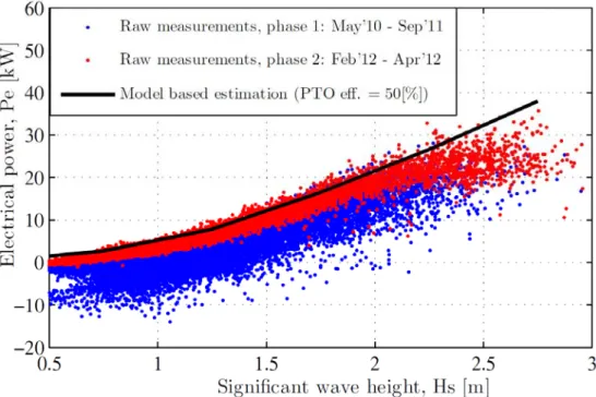
measurements of Wavestar’s prototype during phase 1 (blue dots) and phase 2 (red dots). It is expected

that the electrical power during phase 1 would have lower values than in phase 2 because the control

strategy was not optimized for maximum electrical power (and energy) in phase 1. A significant portion of

the raw measurements from phase 1 are negative. That is, electrical energy is being drawn from the grid.

The results of numerical model simulations of the electrical power at the different wave heights are dis‐

played by the black line (using a typical wave period and direction). It can be seen that up to Hs

≈

2[m] there is a reasonable degree of accuracy between the model and the measurements of phase 2. In Appen‐

dix A it is shown that due to the low water depth at the location the waves are steep and breaking when

the significant wave height is higher than approximately 2.0[m]. Such waves are not ideal for the power

performance and the deviation between the model estimate and the achieved measured maximum power

may be explained by the influence of steep and breaking waves. Taking this into consideration, the model

estimations are in good agreement with the measurements. Hence the model may be used to make ap‐

proximate estimations of the annual generated energy production.

Figure 8: Raw data of electrical power measurements in phase 1 and phase 2. Approx. 18000 data points shown in phase 1 and approx. 8000 data points shown in phase 2. The black line shows the simulation result of the electrical generated power of the WEC with a PTO efficiency of 50[%]. The maximum electrical power measured is approx. 35[kW] at a significant wave height between 2.6[m] and 2.8[m].

(12)

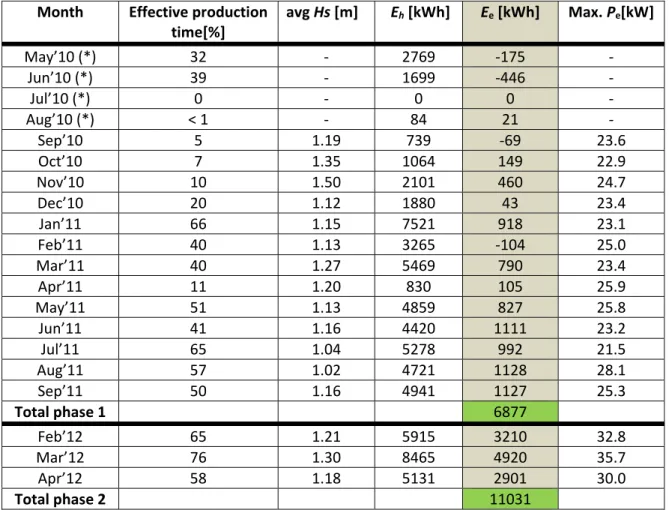
The electrical energy production per month is summarized in Table 6. During phase 1 a total amount of

electrical energy of approx. 7[MWh] was generated while in phase 2, which is a shorter period, the electri‐

cal energy was approx. 11[MWh]. In phase 2 the average effective production time was 66.3[%] and the

average significant wave height during the time with production was 1.23[m].

Month Effective production

time[%] avg Hs [m] Eh [kWh] Ee [kWh] Max. Pe[kW] May’10 (*) 32 ‐ 2769 ‐175 ‐ Jun’10 (*) 39 ‐ 1699 ‐446 ‐ Jul’10 (*) 0 ‐ 0 0 ‐ Aug’10 (*) < 1 ‐ 84 21 ‐ Sep’10 5 1.19 739 ‐69 23.6 Oct’10 7 1.35 1064 149 22.9 Nov’10 10 1.50 2101 460 24.7 Dec’10 20 1.12 1880 43 23.4 Jan’11 66 1.15 7521 918 23.1 Feb’11 40 1.13 3265 ‐104 25.0 Mar’11 40 1.27 5469 790 23.4 Apr’11 11 1.20 830 105 25.9 May’11 51 1.13 4859 827 25.8 Jun’11 41 1.16 4420 1111 23.2 Jul’11 65 1.04 5278 992 21.5 Aug’11 57 1.02 4721 1128 28.1 Sep’11 50 1.16 4941 1127 25.3 Total phase 1 6877 Feb’12 65 1.21 5915 3210 32.8 Mar’12 76 1.30 8465 4920 35.7 Apr’12 58 1.18 5131 2901 30.0 Total phase 2 11031

Table 6: Raw measurements of hydraulic and electrical energy per month. The average significant wave height Hs during the time with production is shown in the third column. The right column of the table shows the maximum elec‐ trical power in average over a 10 minute period. Before February 2012 the control strategy was not optimized for maximum generated energy. Note that effective production time is the result of multiplying the operational time with the production time. Taking June 11 as an example, since the operational time is 92[%] and the production time is 45[%], then the effective production time is 0.92x0.45x100 = 41[%]. That is, 41[%] of the time of a month the machine was in production mode.

In Appendix B the Case 1A model simulations for the Roshage WEC uses the actual PTO efficiency and the

measured wave climate at the site. The simulations show an expected production by the Roshage WEC of

46[MWh/year] which corresponds to 46/4 = 11.5[MWh] in a three month period (taking three months as

an average quarter of a year). It is seen that the estimated electrical energy by the model was only slightly

higher than the actual measured energy during phase 2 of 11.0[MWh]. Taking the wave climate at the site

into consideration the model estimations are in good agreement with the measurements.

(13)

Since the production time varies from month to month it is not possible to directly determine the perfor‐

mance of the control optimization on the electrical energy. In order to better compare the energy values,

the entries in Table 6 are weighted as if the WEC had run an equal effective production time during each

month. The average effective production time shown in the last three months is 66[%]. Taking June 2011 as

an example, if the WEC was in production during 66[%] of the time, the weighted hydraulic and electrical

energy would be Eh[kWh] = ∙ 4420 = 7115 and Ee[kWh] = ∙ 1111 = 1788. Figure 9 shows the result of weighting all the energy entries in Table 6 with a production time of 66[%].

Figure 9: Weighted measurements of the monthly harvested and generated energy of the prototype (weighted with a production time of 66[%]).

It can be observed from Figure 9 that although the hydraulic energy after the control optimization is not

higher than in the previous months, the electrical energy is approximately a factor of two higher, implying

that without increasing the structural load, more energy is generated and a higher PTO efficiency is

achieved as a consequence. In the months before the optimization, the highest PTO efficiency is recorded

in June 2011 with an efficiency of 25[%] and after the optimization the highest PTO efficiency is recorded in

March 2012 with an efficiency of 58[%]. PTO efficiency is here defined as the ratio between the electrical

energy and the hydraulic energy (PTO efficiency = Ee/Eh x 100).

(14)

5

Future

plans

and

activities

The Wavestar prototype at Hanstholm is an ideal test WEC for further development of Wavestar’s concept.

So far the prototype has proved valuable in design validation and based on the experiences with the proto‐

type several modifications to the original design are now being incorporated in the design of future com‐

mercial WEC’s. Building, installing and operating the prototype has provided a unique chance to correct

design errors, which for the prototype was of minor consequence but which for a full converter could have

been a show‐stopper for the concept. Important achievements have been made since the installation of the

prototype, see the timeline for events in Figure 2, Section 2. Being the latest achievement the improved

production time together with a substantial increase of electrical energy produced in phase 2 compared to

phase 1. In order to ensure continuity in Wavestar towards a commercial WEC, a number of activities listed

below have been discussed which could be carried out in the future.

 Autonomous operation of WEC

Since the commercial WEC must be able to operate with a minimal human intervention, it

would be relevant to further increase the degree of autonomy of Wavestar’s prototype.  Upgrade to high efficient PTO

Once new high efficient PTOs that are under development have proved to work as intended,

one or both PTOs in Wavestar’s prototype could be upgraded with the new PTO generation. In

addition of getting a higher WEC efficiency, the PTO could be tested and stressed in real oper‐

ating conditions to gain more knowledge on how it behaves.

 Mechanical optimization and improvement of operational reliability

The mechanical set‐up of the moving arm and cylinder includes bearings, joints and suspen‐

sions which are subject to many motion cycles during the service life. The fatigue life, the oper‐

ational reliability and the maintenance costs could be improved by a more thorough study on

the mechanical set‐up and further real life testing of new materials and components (especially

the cylinder attachments, gyro suspension and bearings, seals and gaskets).



 Installation of new arm and/or float made of concrete

There is an appealing economical reason of producing the arms and/or floats using concrete.

Current studies are being made in order to assess the feasibility of concrete structures and

whether the concrete properties are comparable or better to glass fiber (float) and steel (arm).  Equipping the WEC with additional sensors

By equipping the floats and arms with additional sensors, valuable knowledge on the forces and

motions affecting the floats and arms can be acquired. It gives the possibility to design a more

cost efficient structure and yet ensuring high performance at the desired operation range. Re‐

cently a load cell has been installed in the joint between the cylinder and the arm, and

Wavestar is now in the process of selecting suitable pressure transducers to be equipped on

the outer shell of the floats.

 Further model development and experimental work

A small scale (float diameter of 0.25[m]) test rig has been designed and installed at Aalborg

University with the purpose of investigating in greater details the complex interaction between

the waves and the floats. The experimental results from the new test rig and the further devel‐

opment on non‐linear numerical models are expected to enable predictions of the power per‐

formance of point absorbers operating in high seas [6]. Hereby more suitable control strategies

can be applied permitting higher power output and/or smaller structural stresses. Medium

scale tests (float diameter of 1.0[m]) are also planned for testing at a large indoor wave facility

in Europe. The main focus in these tests will be the impact from slamming forces from steep

and breaking waves on the float shell. These tests will enable a more suitable and economic de‐

(15)

6

References

[1] http://www.fi.dk/filer/publikationer/2010/energi_2010/html/kap03.htm

[2] http://wavestarenergy.com

[3] Wave Star, udmøntning af ForskVE midler til Roshage mole anlægget. 2010‐05‐07.

[4] E. Vidal, R.H. Hansen and M. M. Kramer. ”Early Performance Assessment of the Electrical Output of

Wavestar’s prototype”, International Conference on Ocean Energy, 2012.

[5] R.H. Hansen, T.O. Andersen and H.C. Pedersen. ”Analysis of discrete pressure level systems for Energy

Converters”. Proc. Int Fluid Power and Mechatronics (FPM) Conf, 2011, 552‐558

[6] M. M. Kramer, F. Ferri, A. Zurkinden, E. Vidal and J.P. Kofoed. “Experimental Validation of Numerical

Models for Wave Energy Absorbers”. Structural Design of Wave Energy Devices 2012.

[7] R. H. Hansen and M. M. Kramer, “Modelling and control of the Wavestar prototype”. Proceedings of

the European Wave and Tidal Conference, 2011.

[8] M. M. Kramer, L. Marquis and P. Frigaard, “Performance Evaluation of the Wavestar Prototype”, Pro‐

ceedings of the European Wave and Tidal Conference, 2011.

[9] Danmarks Meteorologiske Institut “Storms in Denmark since 1891”, http://www.dmi.dk/dmi/storme‐

2.pdf, 2012.

[10] E. Tacher and J.V. Tornfeldt Sørensen “Long term wave prediction”. Deliverable D1.1 of the SDWED

project. Draft report by DHI 2012‐01‐18. [11] http://www.hydrosoft.civil.aau.dk/

(16)

Appendix

A

Wave

climate

at

the

location

Wavestar is located on the western side of the Roshage pier at a water depth of approximately 5[m], see

Figure 10. Historic wave measurements from the area were available prior to the installation from a wave

rider located in front of the Hanstholm Harbour at a water depth of approximately 17[m]. As the Wavestar

WEC is located close to the shore by the pier at a low water depth the wave power at this location is small‐

er than what is available further offshore. Figure 11 shows a map of the average wave power in the region.

The wave power decreases significantly as the waves are approaching the shore, decreasing from 9 [kW/m]

at 30[m] depth to 6[kW/m] at 17[m] depth to about 3[kW/m] at 5[m] depth. In other words the available

wave power at the Wavestar location is about the half of what is found at the location of the wave rider.

Since the installation of Wavestar wave recordings at the exact location of the WEC have been recorded by

an ultrasonic wave sensor, see the upper right picture in Figure 11.

Figure 10: Position of Wavestar by Roshage pier and the wave rider in front of the Hanstholm Harbour.

Figure 11: Map showing average wave power (30 year average, figure is from [10]). The upper right picture shows the location of Wavestar by the seaward end of the Roshage pier and the location of the ultrasonic wave sensor.

Hanstholm Wave Rider

20 10 6 Wavestar Wavestar & Ultrasonic Wave Sensor

(17)

The measurements of the waves at the two locations have been analyzed to provide the average annual

wave climate. The wave climate by the Hanstholm Wave Rider is given in Table 7, and the wave climate by

Wavestar is given in Table 8. The frequency table with wave climate at the Wavestar WEC is based on a

complete one year of measurements covering the period for phase 1 and 2 (1 May 2011 to 1 May 2012).

The software package Wavelab developed at Aalborg University has been used to analyze the measure‐

ments from the ultrasonic sensor [11].

Table 7: Frequency table with annual wave climate by the Hanstholm Wave Rider (based on 7 years of 30 minute his‐ toric data). Values inside the table are in [%] of the time.

Table 8: Frequency table with annual wave climate by Wavestar (based on 1 year of 30 minute data from an ultrasonic sensor, 1 May 2011 – 1 May 2012). Values inside the table are in [%] of the time.

The yearly average wave climate at the two locations and the part of time with waves suitable for produc‐

tion is shown in Table 8 and Figure 12 shows the occurrence probability of the waves at the two locations.

It is seen that the waves are small in height and short by the Wavestar location in a higher percentage of

the time and that there is a lower percentage of large and long waves at the Wavestar location. In the fol‐

lowing two sections the reasons for these effects are explained further.

Location

Wave climate Part of time with different wave climate [%]

Significant wave height Wave period Calm sea Storm Production

Hm0 [m] T0,2 [s] (Hm0<0.5m) (Hm0>3.0m) (0.5m<Hm0<3.0m)

Hanstholm Wave Rider 1.24 4.34 13.2 3.4 83.4

Wavestar location 0.88 3.88 27.5 0.0 72.5

Table 9: Overview of annual wave climate by Wavestar and by the Hanstholm Wave Rider.

0-1 1-2 2-3 3-4 4-5 5-6 6-7 7-8 8-9 9-10 0.5 1.5 2.5 3.5 4.5 5.5 6.5 7.5 8.5 9.5 0.0 - 0.5 0.25 2.65 8.18 1.84 0.38 0.14 0.03 0.01 13.23 0.5 - 1.0 0.75 1.22 19.21 11.44 2.21 0.18 0.06 0.02 34.35 1.0 - 1.5 1.25 6.84 13.07 2.96 0.30 0.04 23.21 1.5 - 2.0 1.75 0.33 9.58 3.05 0.29 0.04 13.30 2.0 - 2.5 2.25 0.02 3.34 4.60 0.20 0.04 8.20 2.5 - 3.0 2.75 0.01 0.22 3.89 0.21 0.01 0.01 4.35 3.0 - 3.5 3.25 1.38 0.51 0.01 0.01 1.92 3.5 - 4.0 3.75 0.17 0.57 0.02 0.01 0.78 4.0 - 4.5 4.25 0.24 0.07 0.32 4.5 - 4.75 0.07 0.21 0.05 0.01 0.34 All 3.87 34.60 39.50 18.64 2.72 0.52 0.12 0.04 100.00 Hm0 (m) Hm0 (m) Wave period T0,2 (s) All 0-1 1-2 2-3 3-4 4-5 5-6 6-7 7-8 8-9 9-10 0.5 1.5 2.5 3.5 4.5 5.5 6.5 7.5 8.5 9.5 0.0 - 0.5 0.25 7.88 13.07 5.42 0.93 0.14 0.02 27.45 0.5 - 1.0 0.75 2.59 23.38 11.56 2.39 0.15 40.06 1.0 - 1.5 1.25 8.61 8.48 0.38 17.48 1.5 - 2.0 1.75 0.97 9.12 0.31 10.40 2.0 - 2.5 2.25 0.02 3.87 0.13 4.03 2.5 - 3.0 2.75 0.57 0.01 0.58 3.0 - 3.5 3.25 0.00 3.5 - 4.0 3.75 0.00 4.0 - 4.5 4.25 0.00 4.5 - 4.75 0.00 All 0.00 0.00 10.46 46.05 39.02 4.15 0.29 0.02 0.00 0.00 100.00 All Hm0 (m) Hm0 (m) Wave period T0,2 (s)

(18)

Figure 12: Annual distribution of waves by Wavestar and by the Hanstholm Wave Rider.

A.1.

Reflections

from

the

pier

and

no

production

in

calm

sea

The WEC is placed by the side of the Roshage Pier and waves coming from Eastern directions will therefore

not reach the converter, see Figure 13. As the WEC is often in shelter of the pier there will be a relatively

large percentage of the time with calm sea at the location of the WEC. When Hs is below 0.5[m] the WEC is

out of operation due to calm sea, and as seen in the recorded data the WEC was out of operation in about

25[%] during phase 2:

February 2012 22.3[%]

March 2012 19.1[%]

April 2012 35.0[%]

Figure 13: Position of Wavestar by Roshage with sketch of waves from Eastern and Western directions.

In case of waves coming from Western directions the reflections from the pier gives a more chaotic wave

field between the floats and the pier, see Figure 14. This is preventing an accurate control of the floats, and

thereby a loss in power absorption efficiency.

Waves coming from Eastern

directions are reflected by

the pier and therefore do not

reach Wavestar

N

Waves coming from Western

directions are reflected by

the pier and in this case the

waves by Wavestar are a mix

of incoming and reflected

(19)

Figure 14: Picture showing the chaotic wave field between the floats and the pier in case of waves from West.

A.2.

No

consistent

high

waves

The bathymetry in the area and the low water depth at the location is causing substantial wave breaking

when the significant wave height is exceeding approximately 2.0[m]. A few measurements are available in

the highest recorded sea states with significant wave heights slightly higher than 2.5[m], in which almost all

the individual waves are breaking before or at the structure. It is obvious to visually notice that the wave

breaking with steep wave crests with foam at the top is not ideal for the operation of the WEC and for the

energy production by the WEC, see Figure 15.

Figure 15: Picture showing wave breaking in front of the WEC. The significant wave height is 2.2[m].

The high waves

are breaking in

front of the WEC

Reflections between the

floats and the pier is causing

a chaotic wave field in this

area in case of waves from

(20)

Appendix

B

Production

estimates

by

the

WEC

model

In Section 4 it was demonstrated that there is a reasonable agreement between the measurements and the

model of the WEC. Based on the same model six relevant cases are considered in order to have an estimate

on how a Wavestar machine may perform under different configurations and wave conditions. Three ma‐

chine configurations are considered in Case 1, 2 and 3, and different wave climates are considered in Case A

and B. Details of the estimations are given in the following pages and the results are summarized in Table

10.

Location No. of floats Float diameter [m] PTO eff [%] Production [MWh/year]

Case 1A Roshage 2 5 50 46

Case 1B Hanstholm Wave Rider 2 5 50 73

Case 2A Roshage 20 5 70 589

Case 2B Horns Rev II 20 5 70 873

Case 3A Roshage 20 6 70 804

Case 3B Horns Rev II 20 6 70 1383

Table 10: Summary of the estimated annual production of energy in six different cases.

The main difference between Case 1 and the other cases is that Case 1 deals with a prototype, with two

floats and a PTO efficiency of approx. 50[%], and not with a commercial WEC. Wave Star is currently work‐

ing on a new PTO where conservative estimates indicate that an efficiency of 70[%] from the floats to the

grid should be possible with the potential of an efficiency above 80[%], see [5].

When going into sites with larger water depth than what is present at Roshage Wave Star has done COE

calculations which show better economy for larger machines. This is the reason for configuration Case 3

with larger floats of Ø6[m].

Looking at the production results in Table 10 the following main conclusions are drawn.

Comparing Case 1A with Case 1B:

It is known that the location of the prototype in Roshage is not ideal, see Appendix A, seen from a perfor‐

mance point of view. By placing the same machine in deeper waters by the Hanstholm Wave Rider, a signif‐

icant improvement on the annual production is anticipated. The estimated yearly production is increased

from 46[MWh/year] to 76[MWh/year], corresponding to an increase of (76‐46)/46*100 = 65 %.

A commercial Wavestar WEC with 20 floats of Ø5[m] placed by Roshage will according to the calculations

produce 589[MWh/year], but if the same machine is placed at Horns Rev II it is expected to produce

873[MWh/year], corresponding to an increase of (873‐589)/589*100 = 48 %.

A commercial Wavestar WEC with 20 floats of Ø6[m] placed by Roshage will according to the calculations

produce 804[MWh/year], but if the same machine is placed at Horns Rev II it is expected to produce

1383[MWh/year], corresponding to an increase of (1383‐804)/804*100 = 72 %.

Comparing Case 2B with Case 3B:

A commercial Wavestar WEC with 20 floats placed at Horns Rev II will according to the calculations produce

873[MWh/year] if the floats are Ø5[m], but if the same machine is scaled up to use Ø6[m] floats it is ex‐

(21)

B.1.

Case

1:

Wavestar

prototype

(2

floats

Ø5[m])

Case 1A (Roshage) Case 1B (Hanstholm Wave Rider)

Table 11: Estimated generated energy per year and model parameters for Case 1A (left) & Case 1B (right).

Table 12: Power matrix of generated electrical power for Case 1. Values inside the table are in [kW].

Machine specifications

Production to grid [MWh/year] 46

Float diameter [m] 5

Length of arm [m] 10

Site depth [m] 5

Max control torque e6[Nm] 1

Array interaction [%] 85

Number of floats 2

Main parameters

Site ROSHAGE (may'11-'12)

Machine geometry default

Length of arm [m] Scalable (ref = 10[m])

PTO efficiency [%] 50

Storm protection [m] 3

Secondary parameters

Min. PTO power [kW] 0

Max. PTO power [kW] 110

Background consumption [kW] 0

Part of time in production [%] 95

Main parameters

Site Hanstholm Wave Rider

Machine: Electrical power [kW] 100% operation, array interaction, power limit and storm protection limit Wave period T0,2 [s]. Range and center value on second row.

PTO efficiency [%] Range Center 0-1 1-2 2-3 3-4 4-5 5-6 6-7 7-8 8-9 9-10 10-11 11-12 12-13 13-14 14-15

50 0.5 1.5 2.5 3.5 4.5 5.5 6.5 7.5 8.5 9.5 10.5 11.5 12.5 13.5 14.5 Arm length [m] 0.0 - 0.5 0.25 0 0 0 0 0 0 0 0 0 0 0 0 0 0 0 10 0.5 - 1.0 0.75 0 0 1 2 3 3 3 3 3 3 3 2 2 2 2 Float diameter [m] 1.0 - 1.5 1.25 0 0 3 7 9 9 9 8 8 7 6 6 6 5 5 5 1.5 - 2.0 1.75 0 1 6 13 17 17 16 14 13 12 11 10 10 9 8 Number of floats 2.0 - 2.5 2.25 0 1 10 22 27 26 24 21 19 18 16 15 14 13 12 2 2.5 - 3.0 2.75 0 2 15 33 38 36 32 29 26 24 22 20 18 17 16 Storm protection [m] 3.0 - 3.5 3.25 0 0 0 0 0 0 0 0 0 0 0 0 0 0 0 3.00 3.5 - 4.0 3.75 0 0 0 0 0 0 0 0 0 0 0 0 0 0 0 Nominal power [kW] 4.0 - 4.5 4.25 0 0 0 0 0 0 0 0 0 0 0 0 0 0 0 110 4.5 - 4.75 0 0 0 0 0 0 0 0 0 0 0 0 0 0 0 Hm0 [m]

(22)

B.2.

Case

2:

Wavestar

commercial

machine

(20

floats

Ø5[m])

Case 2A (Roshage) Case 2B (Horns Rev II)

Main parameters

Site depth [m] approx. 15

Main parameters

Site HORNS REV 2

(23)

B.3.

Case

3:

Wavestar

commercial

machine

(20

floats

Ø6[m])

Case 3A (Roshage) Case 3B (Horns Rev II)

Max control torque e6[Nm] 2.1

Main parameters

Site depth [m] approx. 15

Max control torque e6[Nm] 2.1

Main parameters

Site HORNS REV 2