by
Hendrik Mostert Odendaal
Thesis presented in partial fulfilment of the requirements for the degree of
Master of Science in Engineering
at Stellenbosch University
Supervisor: Prof T. Jones
Department Electrical and Electronic Engineering
Declaration
By submitting this thesis electronically, I declare that the entirety of the work contained therein is my own, original work, that I am the sole author thereof (save to the extent expli-citly otherwise stated), that reproduction and publication thereof by Stellenbosch University will not infringe any third party rights and that I have not previously in its entirety or in part submitted it for obtaining any qualification.
October 2012
Copyright © 2012 Stellenbosch University All rights reserved
Abstract
Fault detection and isolation (FDI) is an important aspect of effective fault tolerant control architectures. The Electronic System Laboratory at Stellenbosch University identified the need to study viable methods of FDI. In this research two FDI methods for actuator failures on the Meraka Modular UAV are investigated.
The Meraka Modular UAV is an unmanned aircraft that was developed by the CSIR. A simple six degree of freedom non-linear mathematical model is developed that presents a platform on which the two FDI methods are formulated. The theoretical model is used in a simulation environment to extensively test and compare the performance of the proposed FDI methods in different types of flight conditions.
The first method investigated is a multiple model adaptive estimator (MMAE), which in-corporates a bank of Kalman filters. Each Kalman filter in the MMAE is conditioned for each expected actuator fault scenario. The limitations of using linear Kalman filters are ex-plained and they are replaced by extended Kalman filters, whose associated advantages and disadvantages are discussed. Each filter in the bank of Kalman filters produces a residual vector and residual covariance matrix. This information is subjected to a Bayes classifier to determine the fault scenario which will have the highest likelihood of being active.
The second method that is studied incorporates the parity space approach for FDI. The parity space consists of the parity relations that quantify all the analytical redundancies available between the sensors’ outputs and actuator inputs of a system. A transformation matrix is then optimised to transform these parity relations into residuals that are specially sensitive to specific actuator faults. Actuator faults cause the parity space residuals’ variance to increase. A cumulative summation procedure is used to determine when the residuals’ variance has changed sufficiently to indicate an actuator fault. A pseudoinverse actuator estimation scheme is used to extract the actuator deflections from the parity relations. The FDI performance is tested by deliberately failing specific actuators of the Meraka Modu-lar UAV in-flight. The flight test data is then used to analyse and compare the performance of the two FDI methods investigated in the research. It is found that, for the specific Meraka Modular UAV, the FDI performs as expected with disturbance effects and actuator excitation influencing the FDI effectiveness. The research shows that the bank of Kalman filters creates less false alarms whereas the parity space FDI is more sensitive to faults. It is illustrated that FDI can be improved with active actuator excitation and process noise estimation techniques, delivering promising results.
Uittreksel
Fout-deteksie en -isolasie (FDI) is belangrik vir ’n stelsel se beheerder om foute te kan hanteer. Die Elektroniese Stelsellabaratorium (ESL) by die Universiteit van Stellenbosch het die behoefte geïdentifiseer om te gaan kyk na moontlike FDI-stelsels wat gebruik kan word op hul onbemande vliegtuie (OV). In hierdie navorsing is daar na twee FDI-metodes gekyk wat op die Meraka Modulêre OV toegepas kan word.
Die Meraka Modulêre OV is ’n vliegtuig wat deur die WNNR ontwikkel is. ’n Eenvoudige ses-grade-van-vryheid, nie-liniêre wiskundige model van die Meraka Modulêre OV is ontwikkel, en die FDI-metodes is rondom hierdie model geformuleer. Die teoretiese model is gebruik in ’n simulasie-omgewing en die werkverrigting van die twee FDI-metodes is in verskillende vlug-omstandighede getoets en vergelyk.
Die eerste metode waarna gekyk is, was ’n multi-model aanpasbare afskatter (MMAA), wat ’n bank van Kalman-filters gebruik. Elke Kalman-filter in die MMAA is gekondisioneer vir elke denkbare aktueerder-fout. Die beperkinge rondom liniêre Kalman-filters is uitgelig en vergelyk met uitgebreide Kalman-filters, waarvan die voor- en nadele bespreek is. Elke filter in die MMAA produseer ’n residu-vektor en residu-kovariansiematriks. Hierdie infor-masie is na ’n Bayes-klassifiseerder gestuur om te bepaal watter fout-senario die grootste waarskynlikheid het om aktief te wees.
Die tweede metode waarna gekyk is, het die pariteitsruimte vir FDI gebruik. Die pariteits-ruimte is uit al die pariteitsverwantskappe opgebou wat die verhoudings tussen al die insette en uitsette van ’n sisteem kwantifiseer. ’n Transformasie-matriks is geoptimaliseer om hier-die pariteitsverwantskappe te transformeer na residue wat elkeen sensitief is tot ’n spesikiefe aktueerderfout. ’n Spesifieke aktueerderfout veroorsaak dat ’n spesifieke residu se variansie verhoog. ’n Kummulatiewe sommeringsproses is dan gebruik om te bepaal of die variansie genoegsaam toegeneem het. Sodoende kon daar bepaal word of ’n fout ontstaan het. ’n Pseudo-inversaktueerder-afskattingstegniek is gebruik om die afgeskatte aktueerderdefleksie uit die pariteitsverwantskappe te onttrek.
Die FDI-werkverrigtinge van die twee metodes is getoets deur sekere aktueerders met opset te laat faal gedurende vlugtoetse. Die vlugtoetsdata is gebruik om die werkverrigting van die FDI-metodes te analiseer en met mekaar te vergelyk. Met die spesifieke Meraka Modulêre OV is, soos te wagte, bevind dat versteurings en aktueerderopwekking ’n groot invloed op die FDI’s se werkverrigtinge toon.
Die bevindinge het getoon dat die MMAA-metode minder vals alarms veroorsaak, terwyl die pariteitsruimte meer sensitief vir foute is. Die navorsing toon ook dat die werkverrigting van beide FDI-metodes verbeter kan word met behulp van bykomende aktueerderopwekking en prosesdruisafskattingsmetodes, wat goeie resultate lewer.
Contents
Abstract iii
Uittreksel iv
List of Figures xi
List of Tables xiii
Nomenclature xiv
Acknowledgements xxi
1 Introduction 1
1.1 Background . . . 1
1.2 Preliminary Literature Study . . . 3
1.2.1 Definitions of Fault Tolerant Control and Fault Detection and Isolation 3 1.2.2 Different Theories, Models and Hypotheses . . . 6
1.2.3 Existing Data and Empirical Findings . . . 8
1.2.4 Measuring Techniques and Instruments for Hypotheses Testing . . . . 8
1.3 Research Problem and Objectives . . . 9
1.4 Thesis Outline . . . 10
2 Aircraft Model 12 2.1 Reference Frames Definitions . . . 12
2.1.1 Inertial Reference Frame. . . 12
2.1.2 Body Reference Frame . . . 13
2.1.3 Wind Reference Frame. . . 14
2.2 Notation. . . 14
2.3 Frame Transformations . . . 16
2.3.1 Euler Angles . . . 16
2.3.2 Rotation Matrices . . . 17
2.3.3 Position and Attitude Dynamics . . . 17
2.3.4 Velocity Transformations . . . 18
2.3.5 Quaternions. . . 18
2.4 Assumptions . . . 18
2.5 Equations of Rigid-Body Motion . . . 19
2.5.1 Equations of Forces . . . 19
2.5.2 Equations of Moments . . . 20
2.5.3 General Equations . . . 21
2.6 Aerodynamic Forces and Moments . . . 21
2.7 Gravitational Forces and Moments . . . 23
2.8 Engine Forces and Moments . . . 23
2.9 Change in Aircraft Coefficients . . . 23
2.10 Final Set of Non-Linear Differential Equations . . . 27
2.11 Linearising the Mathematical Model . . . 28
2.12 Discretising the State Space Representation . . . 31
3 First Fault Detection and Isolation Method: A Bank of Kalman Filters 32 3.1 The Fault Detection and Isolation Architecture . . . 32
3.2 Designing the Kalman Filters . . . 33
3.2.1 The Kalman Filter Equations . . . 34
3.2.2 The Kalman Filter for the No-Fault Scenario . . . 35
3.2.3 The Kalman Filters for the Fault Scenarios . . . 36
3.2.4 Replacing the Linear Kalman Filters with Extended Kalman Filters . 37 3.3 Decision Process . . . 38
3.3.1 Gaussian Bayes Classifier . . . 38
3.3.2 State Estimate . . . 41
3.3.3 Final Decision Process . . . 42
3.4 Simulations for the Bank of Kalman Filters FDI Method. . . 42
3.4.1 Simulation Results for a Straight and Level Flight with Minimal Pro-cess Noise . . . 45
3.4.2 Simulation Results for a Straight and Level Flight with Substantial Process Noise . . . 46
3.4.3 Simulation Results for a Circular Flight Path that Closely Resembles the Flight Test Trajectory . . . 47
3.4.4 Simulation Results for a Randomly Generated Flight Mission that Induces Actuator Excitation. . . 48
3.4.5 Simulation Results for a Straight and Level Flight with Minimal Pro-cess Noise, but the Actuators Fail with a Non-Zero Locked-in-Place Fault. . . 49
3.5 Fault Detection and Isolation Performance. . . 51
3.5.1 The Effect of Parameter Changes on FDI Performance . . . 52
3.5.2 The Effect of Process Noise on FDI Performance . . . 53
3.5.3 The Effect of Actuator Excitation on FDI Performance . . . 54
4 Second Fault Detection and Isolation Method: The Parity Space Ap-proach 56 4.1 Parity Relations (Analytical Redundancy) . . . 56
4.3 Optimising the Residuals for Fault Detection and Isolation . . . 61
4.3.1 The Order of the Parity Space . . . 62
4.3.2 The Process Noise Input Matrix . . . 62
4.3.3 The Measurement Noise Input Matrix . . . 63
4.3.4 The Faults Input Matrix. . . 63
4.3.5 Multi-Objective Optimisation . . . 63
4.3.6 Optimisation Technique . . . 65
4.3.7 Optimisation Results. . . 65
4.4 Decision Process . . . 67
4.4.1 The Cumulative Sum Procedure . . . 68
4.4.2 Final Decision Process . . . 69
4.5 Actuator Deflection Estimation . . . 73
4.6 Simulations for the Parity Space FDI Method . . . 74
4.6.1 Simulation Results for a Straight and Level Flight with Minimal Pro-cess Noise . . . 76
4.6.2 Simulation Results for a Straight and Level Flight with Substantial Process Noise. . . 77
4.6.3 Simulation Results for a Circular Flight Path that Closely Resembles the Flight Test Trajectory.. . . 78
4.6.4 Simulation Results for a Random Generated Flight Mission. . . 79
4.6.5 Simulation Results for a Randomly Generated Flight Mission, but the Actuators Fail with a Locked-in-Place Fault of 2.5◦ . . . 80
4.7 Fault Detection and Isolation Performance. . . 82
4.7.1 The Effect of Parameter Changes on FDI Performance . . . 82
4.7.2 The Effect of Process Noise on FDI Performance . . . 82
4.7.3 The Effect of Actuator Excitation on FDI Performance . . . 84
5 Flight Tests 86 5.1 Physical Aircraft . . . 86
5.2 Details of the Flight Tests . . . 88
5.2.1 Wind Conditions . . . 88
5.2.2 Flight Trajectory . . . 89
5.3 Results for the First Flight Test. . . 90
5.3.1 FDI Results Using the Bank of Kalman Filters . . . 90
5.3.2 FDI Results Using Parity Space. . . 93
5.4 Results for the Second Flight Test . . . 95
5.4.1 FDI Results Using the Bank of Kalman Filters . . . 95
5.4.2 FDI Results Using Parity Space. . . 98
6 Comparison of the Two Fault Detection and Isolation Methods 100 6.1 Simulation Results . . . 100
6.1.1 FDI Performance Comparison in Terms of Parameter Change . . . 100
6.1.2 FDI Performance Comparison in Terms of Process Noise . . . 101
6.2 Flight Tests Results . . . 103
6.3 Comparison to Other Literature. . . 105
6.4 Noteworthy Differences. . . 105
7 Recommendations and Conclusion 107 7.1 Recommendations . . . 107
7.1.1 Different Failure Modes . . . 107
7.1.2 Process Noise Estimation . . . 107
7.1.3 Non-Linear Parity Space FDI . . . 108
7.1.4 Practical implementation of the FDI methods . . . 108
7.2 Active Fault Detection and Isolation . . . 108
7.3 Conclusion . . . 111
A Aircraft Parameters: The Meraka Modular UAV 113 B Linearisation 115 B.1 State Matrices . . . 115
B.2 Partial Derivatives of the Elements in the State Matrices. . . 115
B.3 Linearised State Matrices . . . 123
C Process and Measurement Covariance Matrices 124 C.1 Process Noise . . . 125
C.2 Measurement Noise. . . 127
D Healthy and Faulty Residuals Covariance Matrices 128 D.1 Healthy Residuals Covariance Matrices. . . 128
D.2 Faulty Residuals Covariance Matrices Without the Effect of Disturbances . . 128
D.3 Final Faulty Residuals Covariance Matrices . . . 130
E Flight Test Plan 132 E.1 Introduction. . . 133
E.1.1 Background . . . 133
E.1.2 Test Objectives . . . 133
E.1.3 Description of the Test Item. . . 133
E.1.4 Test Scope . . . 133
E.2 Test Preparation . . . 134
E.2.1 Project Team . . . 134
E.2.2 Logistical Support . . . 134
E.2.3 Briefings and Debriefings . . . 134
E.2.4 Safety . . . 134
E.3 Details of the Test . . . 135
E.3.1 Test Conditions. . . 135
E.3.2 Data Required . . . 135
E.3.3 Data Analysis. . . 135
E.4 Test Schedule . . . 136
E.5 Equipment Checklist . . . 137
List of Figures
1.1 Different fault modes. . . 4
1.2 FTC architecture with a FDI and control re-allocation module. . . 5
1.3 Thought process for FDI and control allocation. . . 6
2.1 Inertial reference frame. . . 13
2.2 Body reference frame with velocity notations. . . 13
2.3 Wind reference frame. . . 14
2.4 Body reference frame with force and moment notations. . . 15
2.5 Euler angle transformation sequence (3,2,1) in 3D [1]. . . 16
2.6 Euler angles and the frame transformation. . . 17
2.7 The effect ofαon the aerodynamic coefficient Cd. . . 24
2.8 The effect ofαon the aerodynamic coefficient Cl.. . . 25
2.9 The effect ofβ on the aerodynamic coefficientCY. . . 25
2.10 The effect ofβ on the aerodynamic coefficientCL. . . 26
2.11 The effect ofαon the aerodynamic coefficient CM. . . 26
2.12 The effect ofβ on the aerodynamic coefficientCN. . . 27
3.1 Architecture for the bank of Kalman filters. . . 33
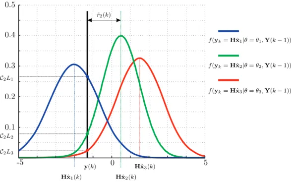
3.2 Conditional probability density for a one-dimensional feature case with three possible fault scenarios. . . 41
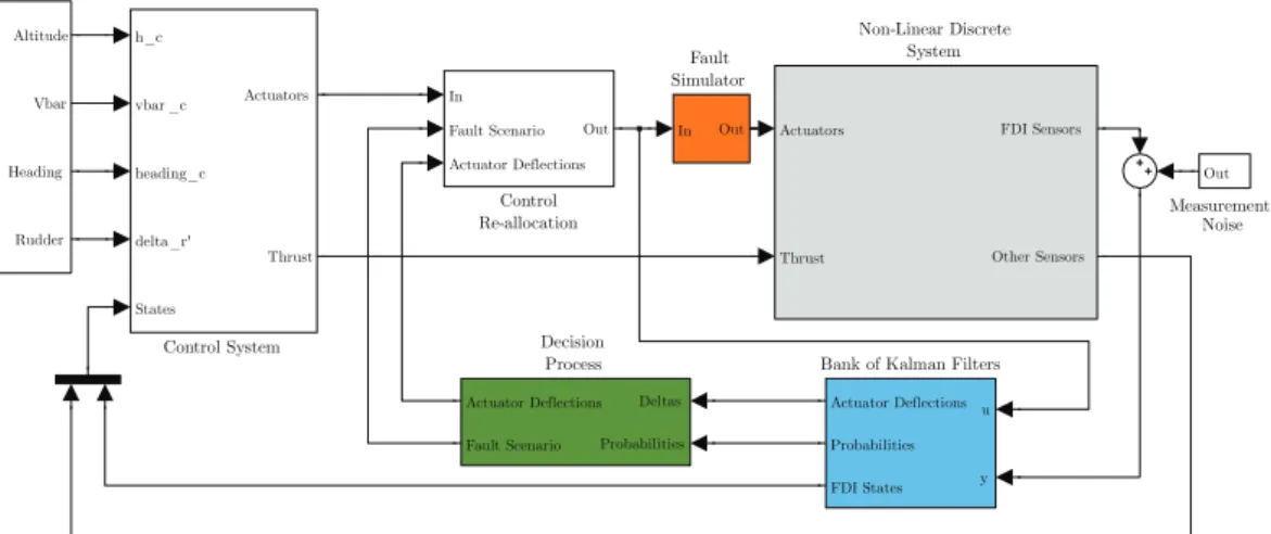
3.3 The Simulink model used to simulate the performance of a bank of Kalman filters for FDI. . . 43
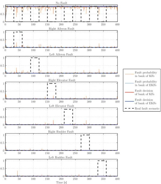
3.4 Probabilities for a straight and level flight with minimal process noise. . . 45
3.5 Probabilities for a straight and level flight with substantial process noise. . . 46
3.6 Probabilities for a circular flight path that closely resembles the flight test tra-jectory. . . 47
3.7 Probabilities for a randomly generated flight mission.. . . 48
3.8 Probabilities for a randomly generated flight mission where the actuators fail with a locked-in-place fault of 2.5◦. . . 49
3.9 Estimated actuator deflections for a random generated flight mission where the actuators fail with a non-zero locked-in-place fault. . . 50
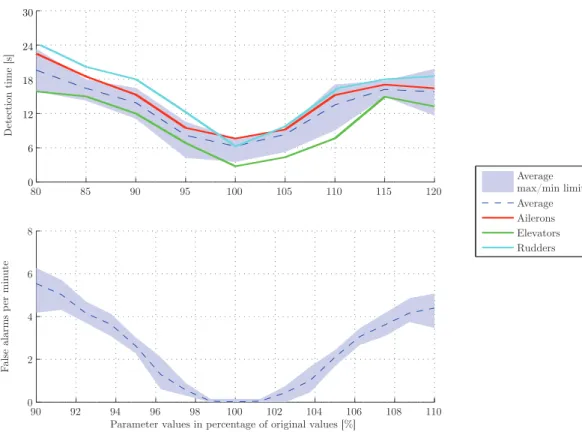
3.10 The effect of parameter changes on the bank of extended Kalman filters FDI performance. . . 52
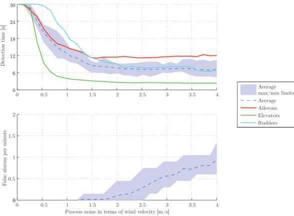
3.11 The effect of process noise on the bank of extended Kalman filters’ FDI
perform-ance. . . 53
3.12 The effect of actuator excitation on the bank of extended Kalman filters’ FDI performance. . . 54
4.1 Conceptual use of the CUSUM procedures to help with the decision process. . . 73
4.2 The Simulink model used to simulate the performance of a parity space FDI method. . . 74
4.3 Fault decisions for a straight and level flight with minimal process noise.. . . 76
4.4 Fault decisions for a straight and level flight with substantial process noise. . . . 77
4.5 Fault decisions for a circular flight path that closely resembles the flight test trajectory. . . 78
4.6 Fault decisions for a randomly generated flight mission. . . 79
4.7 Fault decisions for a randomly generated flight mission where the actuators fail with a locked-in-place fault of 2.5◦. . . 80
4.8 Actuator deflection estimation for a randomly generated flight mission where the actuators fail with a locked-in-place fault of 2.5◦. . . 81
4.9 The effect of parameter changes on the parity space FDI performance. . . 83
4.10 The effect of process noise on the parity space FDI performance. . . 83
4.11 The effect of actuator excitation on the parity space FDI performance. . . 84
5.1 The Meraka Modular UAV. . . 86
5.2 Physical right elevator at−2.5◦ deflection.. . . 87
5.3 Physical right rudder at +2.5◦ deflection. . . 87
5.4 Physical right aileron at +2.5◦ deflection. . . 88
5.5 Maximum and minimum wind gusts. . . 89
5.6 Flight trajectory for both flight tests as seen from above. . . 90
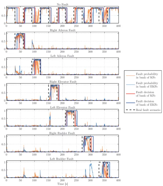
5.7 Fault decisions using the bank of Kalman filters FDI. . . 91
5.8 Actuator deflection estimates using the bank of Kalman filters FDI. . . 92
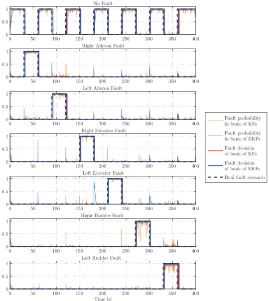
5.9 Fault decisions using parity space FDI.. . . 93
5.10 Actuator deflection estimates using parity space FDI. . . 94
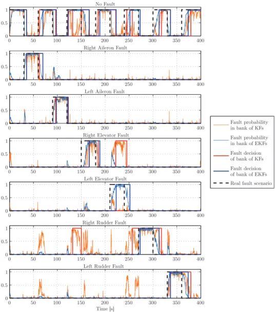
5.11 Fault decisions using the bank of Kalman filters FDI. . . 96
5.12 Actuator deflection estimates using the bank of Kalman filters FDI. . . 97
5.13 Fault decisions using parity space FDI.. . . 98
5.14 Actuator deflection estimates using parity space FDI. . . 99
6.1 FDI performance of the two FDI methods in terms of changing parameter values.100 6.2 FDI performance of the two FDI methods in terms of process noise. . . 101
6.3 FDI performance of the two FDI methods in terms of actuator excitation. . . 102
7.1 The bank of Kalman filters FDI decisions where extra actuator excitation was added. . . 109
List of Tables
3.1 Sequence of fault scenarios in the simulation. . . 44
4.1 Summary of chosen weighting values.. . . 65
5.1 First test flight event summary. . . 90
5.2 Second test flight event summary.. . . 95
6.1 FDI performance of first flight test.. . . 103
6.2 FDI performance of second flight test. . . 104
6.3 FDI performance on the simulations in [2]. . . 105
A.1 Meraka Modular UAV physical parameters. . . 113
A.2 Meraka Modular UAV stability derivatives. . . 114
A.3 Meraka Modular UAV control derivatives. . . 114
E.1 Flight test details. . . 132
E.2 Safety and execution sign-in from. . . 132
E.3 The test schedule. . . 136
E.4 Equipment checklist. . . 137
Nomenclature
Abbreviations and Acronyms
AVL Athena Vortex Lattice
CUSUM Cumulative Sum
CSIR Council for Scientific and Industrial Research
CG Centre of Gravity
CPU Central Processing Unit
DOF Degree Of Freedom
DCM Direction Cosine Matrix
EKF Extended Kalman Filter
EMMAE Extended Multiple Model Adaptive Estimator ESL Electronic Systems Laboratory
FDI Fault Detection and Isolation FTC Fault Tolerant Control GBC Gaussian Bayes Classifier GLR Generalised Likelihood Ratio GPS Global Positioning System
KF Kalman Filter
MIT Massachusetts Institute of Technology MMAE Multiple Model Adaptive Estimator PDF Probability Density Function QFT Quantitative Feedback Theory
RAM Random Access Memory
RMS Root Mean Square
RLS Recursive Least Squares
UAV Unmanned Aerial Vehicle
3D Three-Dimensional
Uppercase Letters
A Wing aspect ratio
A Continuous state matrix
B Continuous input matrix
C Dimensionless aerodynamic coefficients
C Expected shift in variance
C Continuous measurement matrix
D Aircraft displacements along the zI-axis (downwards)
E Aircraft displacements along the yI-axis (east)
F Force vector
F Discretised state matrix
G Discretised input matrix
H Momentum vector
H Discretised measurement matrix
I Mass moment of inertia
I Mass moment of inertia tensor
J Parity space input matrix
K CUSUM “leak” parameter
K Kalman gains
L Aircraft moment along thexb-axis
L Dimension of state vector
L CUSUM detection limit
L Parity space input matrix for process noise, measurement noise or faults
L Likelihood
M Aircraft moment along theyb-axis
M Moment vector
N Aircraft moment along thezb-axis
N Dimension of measurement vector
N Aircraft displacements along the xI-axis (north)
N Sequence of last measurement noise or process noise
N Normal distribution
O Observability matrix
P Aircraft angular rate along thexb-axis
P State estimate covariance matrix
P Sequence of last faults
P Parity relations vector
Q Aircraft angular rate along theyb-axis
Q Process noise covariance matrix R Aircraft angular rate along thezb-axis
R Measurement noise covariance matrix
R Parity space residuals
S Wing (airfoil) area
S Residual covariance matrix
S Parity space input matrices for the process noise, measurement noise or faults
T Thrust
T Length of time step
T Transformation matrix
U Aircraft velocity along the xb-axis (forward)
U Sequence of the last n+ 1 input vectors V Aircraft velocity along the yb-axis (lateral)
V Air flow velocity vector of the aircraft
W Aircraft velocity along the zb-axis (downward force)
X Aircraft forces along thexb-axis (axial force)
Y Sequence of last observed sensor values Z Aircraft forces along thezb-axis (normal force)
Lowercase Letters
b Wing span
c Chord length
c Arbitrary lag time
c Optimisation weightings
c Mean aerodynamic chord
c Directional column vector
e Oswald efficiency factor
f Fault signal
f Probability density
g Gravitational constant
h Altitude above sea
k Time step
m Mass
n Parity space order
p Perturbation of angular rate along thexb-axis
p Probability
p Momentum vector
q Perturbation of angular rate along theyb-axis
q Dynamic pressure
r Perturbation of angular rate along thezb-axis
r Residual
t Time
u Perturbation of velocity along thexb-axis
u Input vector
v Perturbation of velocity along theyb-axis
w Perturbation of velocity along thezb-axis
w Process noise vector
y Measurement vector
x State vector
Subscripts
A Aileron deflection
a Aerodynamic force or moment
b Body reference axes
d0 Static drag coefficient
E Elevator deflection
F Flap deflection
F Faulty covariance matrix
f Faults
g Gravitational force or moment
H Healthy covariance matrix
I Inertial reference axes
k Time step
L Rolling moment coefficient
l Left actuator
l Lift coefficient
l0 Static lift coefficient lα Lift due to angle of attack
lQ Lift due to pitch rate
lδi Lift due to theith actuator
Lβ Roll moment produced by side slip coefficient
LP Roll moment produced due to roll rate perturbations
LR Roll moment produced due to yaw rate perturbations
Lδi Roll moment produced due to theith actuator
M0 Static pitching moment coefficient Mα Pitch stiffness coefficient
MQ Pitch damping coefficient
Mδi Pitching moment produced due to theith actuator
N Yaw moment coefficient
Nβ Yaw moment produced by side slip coefficient
NP Yaw moment produced due to roll rate perturbations
NR Yaw moment produced due to yaw rate perturbations
Nδi Yaw moment produced due to theith actuator
R Rudder deflection
r Right actuator
T Trim
t Thrust force or moment
v Measurement noise
w Wind reference axes
w Process noise
wind Expected wind velocity
wp Working point
X Axial force coefficient
Y Lateral force coefficient
Yβ Side force due to side slip coefficient
YP Side force produced due to roll rate perturbations
YR Side force produced due to yaw rate perturbations
Yδi Side force due to theith actuator
Z Normal force coefficient
Greek Letters
α Angle of attack
β Side slip angle
δ Control actuator vector
Ω Angular velocity vector
Ω Left null space of the observability matrix
µ Multivariate mean vector
Φ Roll rotation angle
φ Perturbation around roll angle
Ψ Yaw rotation angle
ψ Perturbation around yaw angle
ρ Air density
σ Variance
τ Arbitrary lag time
Θ Pitch rotation angle
θ Perturbation around pitch angle
θ Fault scenario
Σ Covariance matrix
Syntax and Style
A The matrix A(usually uppercase)
x The vectorx(usually lowercase) ˆ
x Indicates the estimated value ofx
Acknowledgements
This research would not have been possible without the support and understanding of many people in my life. I would however like to offer my greatest thanks to the following people: First and foremost to my supervisor, professor Thomas Jones, for his experienced guidance and indispensable knowledge. His enthusiastic encouragement has made me able to enjoy completing this research.
I would like to thank Lionel Basson and Anton Runhaar for their valuable assistance in regards to the flight tests and their patience with the Meraka Modular UAV.
Without Ami Philp I would not have had the power and perseverance to complete this research. She supported me in times of doubt and was there in times that I most needed it. Lastly, I would like to thank my friends at the faculty, especially Dirk, Attie, Wikus and Wiaan, for the late night work sessions, immense amounts of coffee and keeping me sane.
Chapter 1
Introduction
1.1
Background
With increased technological advancement over the past century, our reliance on the systems that govern our daily lives has become greater than ever before. Humanity has reached a state in which it cannot operate without the complex systems that supply our energy, transportation, food security and even entertainment. The complexity of these systems necessitates improved reliability of the control systems that manage most of these systems. It is clear that a structure of fault detection is paramount in the pursuit of safety, reliability and performance. One of the emerging industries today is automated systems that totally or partially rely on themselves to achieve these three objectives. In this thesis actuator fault detection and isolation of an automated unmanned aerial vehicle (UAV) will be the subject of research.
UAVs have increasingly been used since the 1990s for important automated tasks in several different industries. These tasks include [2]:
• Inspections of power lines, bridges and dams
• Forest monitoring, fire detection, fire fighting (operation and management) • Sea rescue searches
• Border patrols and law enforcement • Environmental and climate research
• Monitoring traffic and transportation systems • Charting and mapping
• Prospecting
• Crop yield prediction, drought monitoring and spraying of pesticides • Observation of oil and gas pipelines in remote areas
• Tactical reconnaissance and operational support 1
Because of the large economic benefit UAVs have, it becomes apparent that the safety and reliability of these UAVs are vital. Several different schemes are being used to meet these goals. Redundancy and robustness are frequently used but compromises performance. Fault tolerant control (FTC) systems, a fairly new branch of control automation, overcome the need to compromise on performance by adapting the system to the fault that has occurred. These schemes are used not only in the unmanned aerospace industry, but in most modern technological systems that rely on sophisticated control systems. Most of these systems are safety-critical systems such as spacecraft, nuclear power stations, chemical plants, automo-biles and manned aircraft. The aim of fault tolerance is to prevent faults from developing into serious failure, hence increasing the availability of the system and reducing the risk of safety hazards. It is necessary to design control systems that are capable of tolerating potential faults in these systems in order to improve the reliability and availability while providing desirable performance.
In a typical aircraft the pilot or control system can manipulate a set of input mechanisms. These mechanisms, such as the thrust generating engines and control surfaces, are controlled to create moments and forces that ultimately change the states of the aircraft in some desired way. The control surfaces are also commonly referred to as actuators.
A traditional airplane has three independent control actuators: the aileron pair, elevator pair and rudder. These actuators must generate desired moments and forces for which a unique solution for control can be found [3]. However, to increase the reliability, manoeuvrability and survivability of modern airplanes, control actuators are no longer limited to just these three. Many more control actuators have been introduced, as well as the decoupling of the actuator pairs, so that the left and right actuator surfaces can deflect independently. With an increase in the number of redundant actuators, the problem of allocating these controls to achieve the desired moments and forces becomes non-unique. Such redundancy has called for effective control allocation or re-allocation (in case of actuator failures) to optimally distribute the required control moment over available actuators.
A control re-allocation system was developed at Stellenbosch University as a master’s study [3] and it forms an integral part of the fault tolerant control architecture being de-veloped at their Electronics Systems Laboratory (ESL). Control allocation and re-allocation is an important process in a typical fault tolerant control scheme. A faulty actuator degrades the achievable moments and forces that can be created by the set of actuators. The con-trol allocation system minimises the difference between the desired and achievable aircraft performance parameters by optimising the allocation of control effort commanded by the control system to the physical actuators on the aircraft. For the control allocation scheme to work it must know that a fault has occurred and it must know the type of fault, the size of the fault, and which actuators are defective [3].
For an effective control allocation process a reliable fault detection and isolation (FDI) system must be in place to supply the required information. Aircraft can use several costly sensors directly attached to the control surfaces to conduct the FDI process by means of a voting scheme. In recent years it has become common practice to use analytical redundancy to supplement some of the sensors in achieving FDI and so reduce the required costs for
reliable FDI. The topic of this research therefore focuses on actuator fault detection and isolation through the use of analytical redundancy.
1.2
Preliminary Literature Study
The FDI for UAVs is a rich field of research and a review on the literature will be presented in the following categories:
• Definitions of FTC and FDI
• Different theories, models and hypotheses • Existing data and empirical findings
• Measurement techniques and instruments for hypotheses testing
1.2.1
Definitions of Fault Tolerant Control and Fault Detection and
Isolation
Since the research will form part of a fault tolerant control architecture, the definition of a fault tolerant system and the corresponding terminology must be understood. The distinction between a fault and a failure is discussed in [4], where a “fault is an unpermitted deviation of at least one characteristic property (feature) of the system from the acceptable, usual, standard condition” and a “failure is a permanent interruption of a system’s ability to perform a required function under specified operating conditions”.
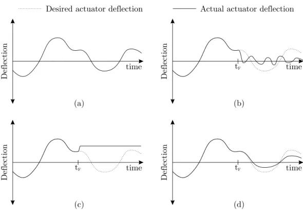
In this research only actuator faults are considered but sensor faults can easily be incorpo-rated into the FDI systems. The reason for this decision is to focus attention on the actuator failure information that is required for the control allocation system. An aircraft has several actuators which may fail at any time on board the aircraft. There are an infinite number of ways in which an actuator can fail. Four of the most common types of operating modes are described below, of which three are failure modes.
(a) No-fault - This mode is the nominal operating mode of an actuator. The actuator follows the desired deflection accurately (figure1.1a).
(b) Floating - The control surface can become detached from the control actuator or can become completely ineffective. This creates a surface that floats around the zero-deflection position (figure1.1b). This can be described as an additive fault.
(c) Locked-in-place - The control surface can become stuck at an arbitrary deflection position (figure1.1c). This can be described as an additive fault.
(d) Effectiveness - The effectiveness of the actuator can become distorted, resulting in a larger or smaller deflection than desired (figure 1.1d). This can be described as an multiplicative fault.
Deflection
time
(a)
Deflection
tF
time
(c)
Deflection
tF
time
(b)
Deflection
tF
time
(d)
Desired actuator deflection
Actual actuator deflection
Figure 1.1: Different fault modes: (a) no-fault; (b) floating fault; (c) locked-in-place fault; (d) effectiveness fault. tF indicates the start of the fault.
Fault tolerant control is a control architecture that is capable of handling a fault or multiple faults while still operating the system at an acceptable performance level. There are several different fault tolerant control schemes that mainly focus on robust control design or adaptive control design. However, for robust control, performance degradation after a fault occurred is a significant issue, whereas for adaptive control, stability assurance is a hurdle [5]. FTC systems usually have several loops in which fault tolerance is applied. In the inner loop an FDI process, which supplies the control allocator with actuator health information, can be used so that the fault affects the performance of the aircraft as little as possible. This is a first defence for faults and will be the method implied in this research. The architecture for this type of first defence FTC is shown in figure1.2. When performance degradation is such that it becomes unacceptable, other fault tolerant processes such as an adaptive controller can be adapted until performance and stability is restored [6].
A more comprehensive bibliographic review on the topic can be found in [7].
Fault detection and isolation systems (also known as a fault detection and diagnosis systems) are concerned with the following three tasks:
1 Fault detection - It is necessary for the system to detect that something has gone wrong, even if it cannot directly determine where the fault is.
Control Re-allocation Plant Controller Desired moments and accelerations Residual Generator Decision Process Unknown disturbances Controlled input Output Fault decision Actuator information Reference Residuals FDI system Figure 1.2: FTC architecture with a FDI and control re-allocation module.
2 Fault isolation - It is the process by which it is determined what part of the system is operating in a faulty manner, for example, “the left elevator is faulty”.
3 Fault identification - The extent of the fault is determined and categorised, for example, “the left flap is stuck at -1.3 degrees” or “the right rudder is floating with an amplitude of two degrees”.
In this research it is of paramount importance to implement all three tasks so that the necessary information can be supplied to the control allocation system. The basic thought process of the desired system after a fault occurs is shown in figure1.3.
As seen in figure1.3, the sensor outputs and control inputs are the only available information from which FDI can be done. These outputs and inputs are used by a residual generator to create residuals. Residuals exhibit specific statistical characteristics that are extracted by calculations of decision statistics. The decision statistics are then used to make a decision about detecting the fault, isolating the fault and identifying the fault. The three respon-sibilities of detection, isolation and identification may be executed in parallel or in series. In some FDI systems, a single detection indicates that a fault is present, as well as its position. The FDI scheme is usually run on-line, in real time. In most systems, the fault detection algorithm is running continuously, while the isolation task is activated only upon the detec-tion of the fault [8]. There are also two families of FDI systems, namely active and passive FDI systems. Active FDI will constantly monitor the system while artificially exciting the UAV [9; 5;10; 11;12] through the aircraft’s actuators. This method decreases the time it takes to detect a fault and can also guarantee fault detection in a set amount of time [13]. The disadvantage of active fault detection is that more energy is used to excite the actua-tors, the actuators wear out faster due to more use, and some level of performance is lost. The second family is passive FDI systems, which also constantly monitor the health of the actuators, but do not artificially excite the actuators to assist the FDI process [14]. Most FDI techniques can be tuned to be either an active or passive FDI system.
Fault identification Fault isolation Decision Residuals Fault detection Normal operation Fault detection and isolation Fault occurs Actuator information New control commands Control re-allocation Normal operation Sensor outputs Actuator inputs Residual generator Calculations of decision statistics Decision statistics Failure decision
Figure 1.3: Thought process for FDI and control allocation.
Some methods and definitions of control allocation are discussed in [6;15;16;17]. There is also a distinction between passive and active FTCs, and [7] is an excellent starting point for a bibliographic review on the topic. More definitions of FTC, FDI and control allocation can be found in [18].
1.2.2
Different Theories, Models and Hypotheses
Several fault tolerant control methods exist and for the research done for this thesis, control re-allocation with a FDI module is the required FTC architecture. An in-depth analysis of the topic is beyond the scope of this study. For a comprehensive list of different FTC methods available, consult [7].
There are also several FDI methods available. These FDI methods can depend on a model based approach or a data based approach. A mathematical model of the aircraft is available and therefore a model based approach is more appropriate for this research. The model based approaches can further be classified by their outcome as a qualitative or quantitative method. A qualitative method can use fuzzy logic or other decision processes to give a measure of fault quality, for example “the left rudder is stuck at a high angle”. The quantitative methods apply numerical values to their decisions such as “the right aileron is stuck at -3 degrees”. The control re-allocation system requires quantitative information to operate and therefore a quantitative method for FDI is an obvious choice.
• State estimation techniques: A fault usually changes the expected state of a system in an additive way. State estimation techniques use the innovations (measurement residual) of the estimators as a means to quantify the discrepancy between the expected behaviour of the system and the observed behaviour. Most faults can be classified as additive and therefore makes this method attractive.
– Observer based approach[19] - The residuals from an observer also qualify for use in an FDI system. There are ways of decoupling disturbances with “unknown input” design methods. The design of the observer can be used to optimise the residuals for FDI as well as to control the observer dynamics.
– Kalman filter (KF) based[20] - A multiple model adaptive estimation (MMAE) technique uses a bank of Kalman filters to estimate the probability of a specific fault scenario. The MMAE method can be applied in practice as long as the expected faults can be hypothesised by a reasonable number of KFs.
• Parameter estimation techniques[21]: Parameter estimation is an intuitive ap-proach of determining multiplicative faults. The dynamic parameters of the system are estimated and compared with the nominal values of a fault-free system model. Parameter Estimation is more reliable than analytical redundancy methods, but it requires more computational power and external excitation.
– Recursive least squares[22] - The Recursive least squares (RLS) filter is an algorithm which recursively finds the filter coefficients that minimize a weighted linear least squares cost function relating to the input signals.
– Regression analysis[21] - The method looks at the relationship between diffe-rent dependent and independent variables to find the best suited set of parameters that describe this relationship. The least square method mentioned above is one of the many regression analysis techniques available for parameter estimation. • Parity space techniques[7]: The parity space relations are the relationships found
between the inputs and outputs of a system and are used as residuals for the FDI system. These relations are obtained from the system’s rearranged mathematical model subject to a linear transformation. The design freedom obtained through the transformation can be used to decouple disturbances and improve fault isolation.
– Input-Output based[8] - If the system can be described by a transfer function relating the output to the input, then residuals can be created with this relation-ship. The limitation of this method is that the number of sensors required must be equal to or more than the number of faults hypothesis to diagnose the faults. This is not the case with redundant actuators on a typical aircraft.
– State space based [23] - The output of a system is a function of the system states, as well as the input to the system. If the null space to the observability matrix can be obtained, then a relationship between the outputs and inputs of the system can be found that is decoupled from the system states. The advantage
of this approach over the basic input-output based approach is that more faults can be diagnosed than the number of sensors on board the aircraft.
1.2.3
Existing Data and Empirical Findings
It is important to test theoretical principles on real-life situations to further our understan-ding of the topic and offer practical solutions to everyday problems. It is also important to compare the work done here with that done internationally so that the significance of this research may be quantified.
The simulation results from most of the techniques discussed above were analysed. For the RLS technique [22] a six-degree-of-freedom, F-16/MATV simulation was run. It shows that the recursive least squares algorithm yields poor results when there is a poorly conditioned observation matrix. It also shows that modifying the RLS to a modified sequential least squares method, improves detection performance considerably.
In [20] it shows that the performance of a bank of Kalman filters (used in a multiple model adaptive estimation scheme) is unacceptable if it is not tuned to some degree. Some of the tuning methods that were proposed are: direct pseudo noise on the process noise covariance matrix’s diagonal elements; direct pseudo noise on the measurement covariance matrix; and tuning for actuator uncertainty. These methods increase the reliability of the detection at the cost of required computing power. Another proposed method is given in [2] where a bank of extended Kalman filters (EKF) is used instead of a bank of linear Kalman filters. The algorithm, combined with an active supervision module, is shown to offer fast and accurate FDI at the expense of additional processing power.
In all of the literature, extensive simulations were performed and in several instances test were done on actual flights. Most methods discussed here used some sort of tuning method or robust technique to enhance the reliability of the specific FDI method. There are also several hybrid systems where more than one technique is incorporated that improves the fault detection abilities. The results of this research are compared with literature in chapter
6.
1.2.4
Measuring Techniques and Instruments for Hypotheses Testing
Accurate simulations can be used as a preliminary measuring tool. In [5] a FTC system is tested on a model that represents the lateral-directional dynamics of a McDonnell F-4C Phantom flying at Mach 0.6 at an altitude of 35 000 ft. Other methods for testing specific signals include the evaluation of the residual vectors in [9] by using a cumulative sum (CUSUM) or a Generalized Likelihood Ratio (GLR) test. MATLAB®is also an excellent simulation tool. The three simulation cases in [24] were performed in MATLAB®6.1 running on a 800 MHz Pentium III computer.
At the ESL MATLAB® R2008b is available on an Intel® Core™i5 CPU @ 2.8 GHz with 4.0 GB RAM. This program will be used extensively to simulate the dynamics of the aircraft and the performance of the FDI methods.
For the practical flight tests in this research a Meraka Modular UAV, that was developed at the Council for Scientific and Industrial Research (CSIR), will be used. The aircraft is equipped with several sensors in its avionics that are used for state estimation purposes. Several of the sensors’ data will be used as an input to the FDI process. The sensors incorporated by the avionics on board the Meraka Modular UAV are:
• Accelerometers & rate gyros - A High Precision tri-axis Inertial Sensor from Analog Devices will be used (model number ADIS16350).
• GPS - A Novatel differential GPS system will be used.
• Angle-of-attack & side-slip angle sensor - The 100400 Mini Air data boom from Space Age Control will be used to measure both the angle of attack and sideslip angles. • Static-pitot tube - The 100400 Mini Air data boom also houses a pitot tube used to
determine the static pressure and the airspeed of the UAV.
The mathematical model and other details of the aircraft will be discussed in chapter2.
1.3
Research Problem and Objectives
There is a need at the ESL for FDI systems for their unmanned automated technology such as the Meraka Modular UAV. The Meraka Modular UAV can be used as a test-bed for the development of a suitable FDI. It should then be possible to use the FDI on other unmanned vehicles by changing a minimum number of parameters. The other vehicles at the ESL will then be able to benefit from the FDI system developed in this research with minimal extra effort.
By creating more than one FDI system the advantages and disadvantages of the systems can be compared, combined and a great deal of understanding can sprout from the evaluation. In section1.2.2it was noted that there are three main methodologies for designing an FDI in a model based, quantitative manner. However the faults that will be focused on are categorised as additive faults (see section 1.2.2) and consequently a parameter estimation methodology cannot be used and leaves only the state estimator and parity space method. One FDI method in each of these two categories will be used to develop independent FDI systems.
The Kalman filter based method is an attractive technique as the estimators aim to produce optimal estimates. Some statistical information regarding the sensors and processes of the aircraft are known and can be used by the Kalman filters. Extended Kalman filters are also used in the state estimation processes incorporated by the ESL on their vehicles. The literature is rich in articles and dissertations covering linear and extended Kalman filter based FDI systems and makes for excellent material for comparison [25].
Both the input-output and state space methods, which fall under the parity space based ap-proach, are covered in [8]. The input-output based method is an excellent FDI development method, but problems arise when more faults can occur than the number of useful detection
sensors. If this is the case the state space based method can be used and allows for more design freedom with the use of optimisation techniques.
The research problem can therefore be stated as the problem of delivering reliable informa-tion regarding the current state of the aircraft actuators. This informainforma-tion can then be used to determine the optimal control allocation for the UAV. The objectives of this research will be categorised as follows:
• Creating two fault detection and isolation systems using two of the techniques men-tioned in the literature review.
• Making both systems usable in the FTC architecture developed in the ESL for the Meraka Modular UAV at Stellenbosch University.
• Testing the system in both a simulation environment and actual test flight environ-ment.
• Analysing and comparing the two FDI methods.
1.4
Thesis Outline
Chapter one gave an introduction to where fault detection and isolation finds itself in the general architecture of a fault tolerant control scheme. A brief literature review covered the basic concepts and philosophies regarding fault tolerant control and fault detection and isolation. The chapter was concluded with the research problem and the objectives of the research.
Chapter two is concerned with deriving the necessary mathematics that will be used in the research. This involves setting up all the required conventions and investigating the dynamics of the Meraka Modular UAV.
Chapter three introduces the development of the first FDI process that incorporates the use of a bank of Kalman filters. The linear Kalman filters will also be replaced by extended Kal-man filters, thereby improving the FDI system. The chapter will conclude with simulation results that show the expected performance of the bank of Kalman filters FDI method. Chapter four describes the development of the second FDI process that uses a parity space approach to create the residuals that will be used for FDI. The method will be optimised for fault detection and isolation whereafter a CUSUM procedure will be introduced, which assists the decision making process. Finally performance simulations and conclusions re-garding this method are presented.
Chapter five is concerned with the test flight conducted at the Helderberg Radio Flyers Club, which tested the performance of both the FDI methods. The physical aircraft actuators and their effects on the expected performance of the FDI are also discussed in this chapter. Chapter six compares the two FDI methods and draws conclusions from the simulated results and flight tests that were conducted. Lastly, the FDI performance is compared to other literature simulations.
Chapter seven provides valuable recommendations regarding practical considerations and proposed future research and applications. The research conclusions completes the end of the thesis.
Chapter 2
Aircraft Model
For a quantitative model based FDI approach, a transfer function or state space repre-sentation of the aircraft is required. In order to obtain this, it is first necessary to obtain the equations of motion for the aircraft. To derive the non-linear aircraft model, specific assumptions must be made and several reference frames defined. In this chapter the inertial, body and wind frames, as well as the gravitational, aerodynamic and thrust model used to describe the non-linear aircraft dynamics for the Meraka Modular UAV, will be defined.
2.1
Reference Frames Definitions
There are three reference frames that must be defined in order to develop a simple six degree of freedom, non-linear model for the aircraft dynamics [26]. The first is the inertial reference frame in which the laws of Newton are applicable. The second is the body reference frame that coincides with the aircraft frame, and lastly the wind frame that describes the direction of airflow over the body of the aircraft.
2.1.1
Inertial Reference Frame
In this research, the earth will be regarded as flat and non-rotating and can therefore be regarded as an inertial reference frame. This is an acceptable approximation as the motion of the Modular UAV will be localised and be relatively slow (22 m/s). This simplifies the dynamic model for the aircraft quite substantially without significant loss of accuracy [3] for the purpose of FDI. The frame is defined as fixed to the earth at some convenient location such as the starting centre of gravity (CG) point of the aircraft before take-off. The x-axis is pointed north, whereas the y-axis points east and the z-axis points downwards to complete the right-hand convention. This definition is depicted in figure 2.1. The subscript used for the inertial reference frame will beI.
Figure 2.1: Inertial reference frame.
2.1.2
Body Reference Frame
The body reference frame is required so that the forces and moments can be mapped in a logical manner to the resulting motions of the aircraft. The centre point of the frame coincides with the CG of the aircraft. This is not always the case, but it is generally placed at the CG and will be done this way in this research.
The x-axis points forward and comes out the nose of the aircraft, while the y-axis points out along the right wing as seen in figure2.2. It must be noted that the x-axis does not coincide with one of the principal axes of the aircraft. Instead it coincides with the originally aligned equilibrium direction of the velocity vector of the aircraft [27]. The z-axis completes the right-hand convention by pointing downwards so that thexb-zb-plane is the aircraft’s plane
of symmetry. The convention is also shown in figure2.2. The subscript used for the body reference frame will be b.
2.1.3
Wind Reference Frame
The wind frame is sometimes also referred to as the stability frame or the aerodynamic frame [28]. The aerodynamic forces that act on the body of the aircraft are produced by the air flowing over the airframe. The air flow velocity is described byVand the direction ofV can be described by two angles relative to the body frame of the aircraft. The two angles are the angle of attack, α, and side slip angle, β. These angles parameterises the change in the air flow pattern over the airframe that consequently produces different aerodynamic forces and moments.
Figure 2.3: Wind reference frame, angle of attack and side slip angle,α> 0 andβ> 0.
The wind reference frame can be defined by lining up thexw-axis with the velocity vector,
V. As shown in figure 2.3 the angle of attack (α) is the angle between the projection of V onto the xb-zb-plane and the xb-axis. The side slip angle (β) is the angle between the
projection of the airspeed vector V onto the xb-zb-plane and the airspeed vector itself [2].
The y-axis and z-axis of the wind reference frame are directed according to these angles as illustrated in figure2.3. The subscript used for the wind reference frame will bew.
2.2
Notation
The components of the total instantaneous values of the linear velocities resolved into the body reference frame are
• U - Forward velocity
• V - Lateral velocity
• W - Downward velocity
• P - Angular rate around thexb-axis
• Q- Angular rate around theyb-axis
• R- Angular rate around thezb-axis
These vectors are shown in figure 2.2.
The notation that will be used for the forces and moments acting on the body of the aircraft is provided in figure2.4. The forces are
• X - Axial force • Y - Lateral force • Z - Normal force and the moments are
• L - Rolling moment • M - Pitching moment • N - Yawing moment
There are eight control surfaces consisting of two ailerons, two flaps, two rudders and two elevators. The control surface deflection angles areδA, δE, δF, δRrespectively. A distinction
will be made between the left and right actuator by adding anlor rsuffix to the subscript according to whether it is left or right (such asδAris the right aileron) as seen from behind
the aircraft. Figure 2.4 shows the control surfaces and their deflections, where a negative deflection causes a positive moment around the body reference frame.
Figure 2.5: Euler angle transformation sequence (3,2,1) in 3D [1].
2.3
Frame Transformations
The aerodynamics of the aircraft are best described in the wind reference frame while the gravitational forces and thrust are described better in the body frame. The position and attitude of the aircraft are however expressed in the inertial reference frame. It is therefore important that vectors should be able to be mapped from one reference frame to another. There are several methods to accomplish this, but three methods worth noting are by using rotation matrices, Euler angles and quaternions. In this research, Euler angles will be used and converted to rotation matrices. Quaternions have benefits (see section 2.3.5) but the control system for the Meraka Modular UAV was developed without their use and subsequently will not be used for the FDI system.
2.3.1
Euler Angles
Using Euler angles is a simple and understandable method used for frame transformation and is therefore a popular choice [1]. The Euler angle transformation is parameterised by three consecutive rotations. There are several different possible non-commutable rotation sequences to describe a specific transformation. The sequence that will be used in this research is the Euler 3-2-1 rotation sequence. This sequence is the same as what is used in the other systems developed at the ESL [3].
In the case of the aircraft attitude the inertial reference frame will be the starting frame and the body frame of the aircraft will be the transformed frame. The angles Ψ, Θ and Φ are called the yaw, pitch and roll angles respectively and they are displayed in figure 2.6
in order of rotation sequence from left to right. This parameterisation has singularities at pitch values of Θ =nπ+π2 forn∈Z[1]. At these points, changes in yaw and roll constitute the same motion. This should however not be problematic in the context of this research as it is assumed that the aircraft stays within|Θ| π
Figure 2.6: Euler angles and the frame transformation.
2.3.2
Rotation Matrices
The Euler angles described in section 2.3.1are helpful but do not work well with column vectors. To solve this problem Euler angles are converted to rotation matrices that can readily be applied to column vectors to transform them from one reference frame to another. When cI is taken as a column vector in the inertial reference frame and cb is taken as a
column vector in the body reference frame, the Euler 3-2-1 sequence is realised by [1]
cI =R321cb (2.3.1) where R321= cΘcΨ cΘsΨ −sΘ sΦsΘcΨ−cΦsΨ sΦsΘsΨ+cΦcΨ cΘsΦ cΦsΘcΨ+sΦsΨ cΦsΘsΨ−sΦcΨ cΘcΦ (2.3.2) andsx= sinx (2.3.3) cx= cosx (2.3.4)
The matrix R321 is also called the direction cosine matrix (DCM). It is shown in [1] that the inverse ofR321transforms the body frame to the inertial frame and that the inverse is also equal to its transpose.
2.3.3
Position and Attitude Dynamics
The position of the airplane can be described by the aircraft’s North, East and downward position. The dynamics of these positions are given by [29]
˙ N ˙ E ˙ D = cΨcΘ cΨsΘsΦ−sΨcΦ cΨsΘcΦ+sΨsΦ sΨcΘ sΨsΘsΦ+cΨcΦ sΨsΘcΦ−cΨsΦ −sΘ cΘsΦ cΘcΦ U V W (2.3.5) where cx= cosx (2.3.6) sx= sinx (2.3.7)
The time rate of change of the Euler angles with respect to the other kinematic states are governed by the derivation found in [26] as
˙ Φ ˙ Θ ˙ Ψ =
1 sin Φ tan Θ cos Φ tan Θ
0 cos Φ −sin Φ
0 sin Φ sec Θ cos Φ sec Θ
P Q R Θ6=nπ+ π 2 n∈Z (2.3.8)
2.3.4
Velocity Transformations
It is helpful to break down the velocity vectorVinto its body-referenced components using the angle of attack and side slip angles, and vice versa. The components can be determined by investigating figure2.3as U V W = cos(β) cos(α) cos(β) sin(α) sin(β) |V| (2.3.9)
and vice versa
α = arctan WU β = arctan VUcos(α)
)
U 6= 0 (2.3.10)
2.3.5
Quaternions
An unwanted consequence of using Euler angles is the singularity at Θ =nπ+π2 forn∈Z.
Quaternions are superior to Euler angles in that they do not display this singularity; however a quaternion transformation between two reference frames is described by four parameters instead of three. As stated previously, quaternions will not be used in this research, so that it conforms to the systems being developed for the Meraka Modular UAV at the ESL. In [1] it is shown that quaternions, Euler angles and rotation matrices can be used interchangeably should the need arise to do so.
2.4
Assumptions
There are six assumptions that must be made before deriving the equations of motion [27]: 1. The axes xb and zb lie in the plane of symmetry of the aircraft and the products of
inertia Ixy and Iyz are equal to zero. The direction of xb is generally not along a
principal axis, hence Ixz 6= 0. For the aircraft used in this research however, the
inertia tensor elementIxz is negligible compared to the rest of the elements.
2. The mass of the aircraft remains constant throughout the dynamic analysis. In practice this is not true as there can be cargo such as equipment, ammunition and projectiles loading and unloading during the course of the flight. There is also the inevitable consumption of fuel in most aircraft that reduces the mass of the aircraft during flight. The Meraka Modular UAV uses battery powered motors and no in-flight loading or unloading is done. Therefore the assumption of constant mass is accurate.
3. The aircraft is a rigid body. This means that any two points on or within the aircraft will remain stationary relative to one another. This greatly simplifies the equations of motion.
4. The earth is an inertial reference, and unless otherwise stated, the atmosphere is fixed with respect to the earth. This assumption is valid for the purpose of this research as it is generally accepted that the gyros and accelerometers on the aircraft cannot discern the angular velocity or accelerations of the earth (not to be confused with gravitational acceleration).
5. The perturbations from equilibrium state are small. With this assumption products of small variations can be ignored and small angle assumptions can be made for the relative angles between the equilibrium and disturbed axes. This assumption has been very successful in simplifying the linearisation process without too much loss of accuracy [26].
6. The airflow over the body of the aircraft is quasi-steady. Quasi-steady flow assumes the airflow changes instantaneously when the aircraft is disturbed from its equilibrium. This assumption is adequate for low Mach numbers (<0.8) and allows all derivatives with respect to the rates of change of velocities to be omitted when setting up an aerodynamic model of the aircraft.
2.5
Equations of Rigid-Body Motion
In the development of the equations of rigid-body motion, the assumption will be made that the aircraft will be flying in a localised area at low velocity. The flat-earth, non-rotating inertial reference frame simplifies these equations as the effects due to the Coriolis acceleration and centripetal acceleration of the earth can be ignored. In the inertial reference frame the laws of Newton apply.
2.5.1
Equations of Forces
The translation of a rigid body is described by its momentum. Newton’s second law relates the change of momentum (the product of the velocity of its CG and its mass) to an external force acting on the body. This is stated as: the summation of all the forces acting on a rigid body equals the time rate of change of its momentum [30]. It can be written as
X j Fj = dpb dt I (2.5.1) = d dt(mVb)I (2.5.2)
wherej represents all the forces acting on the aircraft andpb is the momentum. The forces
equation2.5.2in terms of the body reference frame. The relation then becomes [30] X j Fj = d dt(mVb)b+Ωb×pb (2.5.3) = d dt(mVb)b+Ωb×(mVb) (2.5.4) where Ωb is the angular velocity vector of the aircraft.
2.5.2
Equations of Moments
The rotation of a rigid body is described by its angular motion. Newton’s second law can be used to relate the change in angular velocity to the sum of external moments acting on the aircraft body. This can be more formally stated as: the summation of all the moments acting on a rigid body equals the time rate of change of its angular momentum [30]. It can be written as X j Mj = dH b dt I (2.5.5) = d dt(ΩIb)I (2.5.6)
where Hb is the angular momentum and the angular rate vector
Ω= P Q R (2.5.7)
andIb is the mass moment of inertia tensor that is written as
Ib= Ixx −Ixy −Ixz −Iyz Iyy −Iyz −Izx −Izy Izz (2.5.8)
According to the first assumption from section2.4, the inertia tensor can be greatly simplified into the diagonal matrix
Ib= Ixx 0 0 0 Iyy 0 0 0 Izz (2.5.9)
For the same reason as with the external forces, it would be convenient to write equation
2.5.6in terms of the body reference frame. The relation then becomes [30]
X j Mj = dH b dt b +Ωb×(Hb) (2.5.10) = d dt(ΩIb)b+Ωb×(ΩbIb) (2.5.11)
2.5.3
General Equations
The two equations (Eq. 2.5.4and Eq. 2.5.11) are written in vector form. If the assumption holds for a symmetrical aircraft body around the xb-zb-plane, these two equations can be
expanded into their scalar forms to produce
X =m( ˙U+W Q−V R) (2.5.12) Y =m( ˙V +U R−W P) (2.5.13) Z=m( ˙W+V P−U Q) (2.5.14) L= ˙P Ixx+QR(Izz−Iyy) (2.5.15) M = ˙QIyy+P R(Ixx−Izz) (2.5.16) N = ˙RIzz+P Q(Iyy−Ixx) (2.5.17)
Each of the equations2.5.12to2.5.17are composed of aerodynamic, thrust and gravitational forces and moments so that
X=Xa+Xt+Xg (2.5.18) Y =Ya+Yt+Yg (2.5.19) Z=Za+Zt+Zg (2.5.20) L=La+Lt+Lg (2.5.21) M =Ma+Mt+Mg (2.5.22) L=La+Nt+Ng (2.5.23)
2.6
Aerodynamic Forces and Moments
In this research it is assumed that the aerodynamic stability and control derivatives will be made available by the system identification process running on the aircraft’s computer or from off-line parameter estimation techniques. Therefore the research will not be accom-panied by an in-depth analysis of these derivatives. Further reading on this topic can be found in [3;31; 28; 26;27]. However, a brief explanation of the analysis will be presented. Aerodynamic forces and moments are produced by a pressure difference over the airfoils of the aircraft. Actuators assist in changing the airflow over the airfoil surface to induce certain desired forces and moments. Because air pressure is the driving force behind these dynamics, Bernoulli’s equation and the continuity