Stream-based Active Learning for Efficient and Adaptive Classification of 3D Objects

Stream-based Active Learning for

Efficient and Adaptive Classification of 3D Objects

Alexander Narr

_{Rudolph Triebel}

_{Daniel Cremers}

Abstract— We present a new Active Learning approach for classifying objects from streams of 3D point cloud data. The major problems here are the non-uniform occurence of class instances and the unbalanced numbers of samples per class. We show that standard online learning methods based on decision trees perform comparably bad for such data streams, which are however particularly relevant for mobile robots that need to learn semantics persistently. To address this, we use Mondrian forests (MF), a recent online learning algorithm that is independent on the data order. We present an extension of that algorithm and show that MF are less overconfident than standard Random Forests. In experiments on the KITTI benchmark, we show that this leads to a substantially improved classification performance for data streams, rendering our ap-proach very attractive for lifelong robot learning applications.

I. INTRODUCTION

One major requirement for most modern robotic systems is their ability to extract semantic information from their observed input data. In general, semantic information can be represented in many different ways, including drivable and non-drivable areas for outdoor robots [1], annotated road maps with lanes, intersections and road signs for self-driving cars [2], or the position and orientation of door knobs, hinges of doors for robots with manipulators [3]. In this work, we focus on class labels of road participants such as cars, pedestrians, or cyclists, although our approach can also be used for other applications. The main idea is that of persistent learning, i.e. the robot learns semantics with new observations during operation and not from a previously manually annotated data set. The benefits of this are two-fold: first, the robot is able to adapt to new situations as new observations directly modify its internal representations. And second, learning is done mainly on those observations that actually occur in the robot’s environment and not on the much larger set ofpotentialobservations, i.e. it can be done more efficiently.

However, as we will show in this paper, these benefits come with a major difficulty: in contrast to an offline recorded training data set, data that is perceived online is highly correlated to previous observations. For example, an autonomous car driving on a highway may observe many other cars or motor cycles from many different view points, which can all be added to a large, growing training data set. This leads to a large, but very unbalanced data set, because other road participants such as cyclists or pedestrians

1_{Computer Vision Group, Dep. of Computer Science, TU Munich, 85748} Garching, Germany [narr,triebel,cremers]@in.tum.de

2_{Institute of Robotics and Mechatronics, Dep. of Perception and} Cog-nition, German Aerospace Center (DLR), 82234 Weßling, Germany

[email protected]

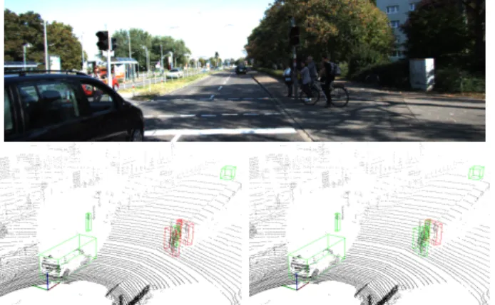
Fig. 1. Example situation from the KITTI benchmark data set with a car, a cyclist and some pedestrians. The 3D point cloud data of this frame was classified after actively learning semantics from a stream of 10 000 previous samples. The bottom left image shows the result from actively learning an online Random Forest classifier, the right one shows the result using a modified Mondrian forest instead. A green bounding box refers to a correct classification, while red boxes are wrong predictions. As we show in this paper, the better performance of Mondrian forests comes from their higher capability to learn from streams of data.

are under-represented. As a consequence, identifying new observations as instances of an unknown object class on appearance is very hard, because standard online learning methods are only able to specialize, but not generalize their models with new data samples and therefore require many samples from the new class. In the literature on Active Learning, this is known as the distinction between pool-basedandstream-basedlearning. To address these problems, we propose an Active Learning framework that uses a more informed and more flexible classification algorithm based on a recent machine learning method. The so-calledMondrian foresthas the major benefit that it is independent on the order in which the data appears, and that it can handle unbalanced data sets much better because its representation does not actually depend on the ground truth class labels. As we show experimentally, this leads to much steeper learning curves even for the stream-based learning scenario.

Our work consists of three major contributions: First, we provide modifications to the original Mondrian forest algorithm, which lead to a better classification performance. Second, we analyze Mondrian forests regarding their ten-dency to make wrong predictions with low uncertainty, i.e. their overconfidence, and we show that Mondrian forests tend to be less overconfident than standard online random forests. And third, we exploit this by setting up an active learning framework using Mondrian forests as underlying

classifier. We show experimentally that this new Active Learning method produces less label queries at a higher prediction accuracy compared to online Random Forests, and that it is particularly well suited for stream-based learning problems such as those often encountered in robotics.

II. RELATEDWORK

Our work has links to three different learning concepts: incremental learning, online learning and Active Learning. Incremental learning refers to “any online learning process that learns the same model as [it] would be learnt by a batch learning algorithm” [4]. Essentially, this means that it can incorporate additional information from newly observed data, e.g. new object classes. Thus, the benefit over offline learning is that incremental learning requires less computation steps when new data is available. An example of an incremental learning method is Learn++ [5], an extension of AdaBoost. The idea is to generate new hypotheses from additional batches of training data and to update the ensemble of weak classifiers accordingly. Another incremental method are nearest class mean forests (NCMF) [6]. They consist of random forests where the decision nodes are based on nearest class mean classifiers [7]. In contrast to other random forests, NCMFs are able to add new classes, because they store parts of the underlying distribution of the feature space in each node. Another popular incremental learning approach is based on one-class Support Vector Machines (SVMs) [8], [9]. The key idea is that the current SVM model is updated on the new data and the support vectors from the previous learning step. The main drawback with all incremental learning methods is however, that they do not provide a functionality to update the learned model from a single new data observation, and they often require to store at least a large fraction of the training data.

In contrast, online learning methods only use the infor-mation from the next data sample, and they do not need to re-use any of the previously observed samples. Recent examples of online learning methods are given by the work of Saffari et al. [10], who introduced online multi-class Gradient Boost and online multi-class LP Boost. In contrast to offline boosting, an online boosting method has a fixed number of weak classifiers and the weak learners themselves are online algorithms, for example online Random Forests (ORF) [11]. The performance of these methods is very good, but as we will show in the experiments, they have problems when the training data is un-balanced.

Finally, our work makes use of an Active Learning frame-work. A good overview of this topic is given by Settles [12]. Some applications of Active Learning include the work of Kapooret al.[13], who perform object categorization using a Gaussian Process classifier (GPC), the work of Vezhnevets

et al.[14], as well as that of Wanget al.[15] who use active learning for interactive image segmentation. In contrast to all these approaches, we address the problem of stream-based Active Learning as opposed to pool-based learning. More details are given below.

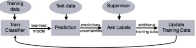
Fig. 2. Generic Active Learning. Starting with an initial training round, new test data are classified, resulting in label predictions and corresponding uncertainties. Based on these, a human supervisor is asked for ground truth labels, and these are joind with the current training data. Then, training is repeated with the extended training data until a stopping criterion is met.

III. PERSISTENTLEARNING FORMOBILEROBOTS

Our goal is to develop an algorithm that learns semantic information (e.g. object class labels) from a large input data set in such a way that ita)adapts its internal representation to new, unseen environments,b) only requires few interactions with a human supervisor (“teacher”) andc)only costs little computational effort when considering a new data sample. The motivation for these aims arises from the intended application in mobile robotics: robots that persistently learn semantics must be able to cope with new situations, should only ask a human when necessary (thereby increasing their level of autonomy), and perform the required computations fast enough to not block the functionality of the whole system. To address the first two goals, researchers have investigated active learning methods, and we will briefly explain this in the following. The third goal refers to the capability for online computation, i.e. to update the repre-sentation without having to re-consider previously observed data samples. In the following, we give some examples for existing online learning methods. Finally, we highlight the major difference of active learning for mobile robots as opposed to other applications such as computer vision and explain the typical drawbacks of standard online learning methods for our purpose. This will motivate our proposed approach presented in Sec. IV.

A. Active Learning

Fig. 2 shows a schematic flow of a generic active learning framework. It starts with an initial training set (_X0,Y0), where_X0 = {x1, . . . ,xN} are N observations represented

asd-dimensional vectors and_Y0={y1, . . . , yN}are ground

truth class labels, i.e.yi2{1, . . . , C} withC 2. Then, in

each learning round orepochj = 0,1, . . ., a classifierfj is

trained using(Xj,Yj). This gives a mappingfj :Rd!RC

that assigns a predictionp2RC_{to each input sample. Next,}

a set of new observationsX⇤

j ={x⇤1, . . . ,x⇤K} is considered and classified using fj. The result are prediction vectors {p⇤1, . . . ,p⇤K}. The key step is then to select a sub set ofXj⇤

for a query of corresponding ground truth labels. A common selection method uses the prediction uncertainties to decide whether a query is triggered. From this query, new ground truth labelsY⇤

j are obtained and, together with the selected

observations, they are added to the current training data set

(_Xj,Yj). The resulting set(Xj+1,Yj+1)is then used to train the classifierfj+1 in the next epoch.

B. Online Learning

In principle, active learning can be performed with any classification algorithm that is capable of providing uncer-tainty estimates with class predictions for new samples. However, in terms of efficiency standard offline learning is not good for Active Learning, because it requires re-training on all the data observed so far in every epoch. As a consequence, the time needed for learning steadily increases and all observed data samples must be kept in memory. Therefore, online algorithms for learning are much more useful. In the literature, many standard offline classification methods have been converted into online methods, but one remarkable contribution is the work of Saffari et al. [10], which provides very efficient online multi-class learning methods based on boosting. The key element in that work is an online Random Forest, which is used as a weak classifier in boosting. An online Random Forest combines online bagging, random feature selection and the growing strategy of extremely randomized trees [16], where the test functions and thresholds are generated randomly. In contrast to an offline node, an online decision node has to see a minimum number ↵ of samples before splitting and a split has to

achieve a minimum gain . For data sets that are roughly uniformly sampled across the classes, this gives comparably good classification results, but for non-uniform data and for data streams this causes problems, as explained below.

C. Pool-based vs. Stream-based Learning

When we described the Active Learning framework, we deliberately did not specify the way in which the test data set_X⇤ _{is given. In principle, there are two ways to do this:}

either_X⇤_{is a fixed-size set of observations that are collected}

beforehand, or it consists of a growing number of samples that are continously observed and added toX⇤_{. Thus, in the}

first case we have a fixedpoolof data, and the algorithm can pick good samples to query from this pool, which is usually very large. This is the most common application for Active Learning. However, in mobile robotics, and in particular for robots that are to learn semantics persistently, the second scenario known as stream-based Active Learning is much more relevant, because robots perceive streams of data, and they should be able to learn from it continously. Therefore, in this paper we consider stream-based Active Learning.

To highlight this distinction further, we performed the fol-lowing experiment. We considered a large, standard bench-mark data set and applied two online classification methods: online Random Forests (ORF) and online multi-class Gra-dient Boost (OMCGB) with ORF as weak classifiers (for both methods see [10]). Then, we resampled the data in such a way that the occurence of samples in each class was distributed uniformly over the time line (see Fig. 3, left and center) and applied again the online classification methods. Evaluation was done on a hold-out set not used for training, and we choose the KITTI data [17] for this experiment (for more details on the used data set we refer to the description in Sec. V-A). The resulting learning curves are shown in the right plot of Fig. 3. As we can see, both

Fig. 4. Comparison between a decision tree and a Mondrian tree for a toy example with three different classes (Figure inspired by [18]). The feature space is defined in[0,1]2_wherex

1andx2denote horizontal and vertical axes.Top:The partition of the space of a decision tree with two axis aligned splits atx1 = 0.55andx2 = 0.65.Bottom:Embedded partition of the space of a Mondrian tree where each node has an associated split time, and the splits are committed only within the range of each sub tree.

online learning methods perform resonably well for the case of uniform distributions of class occurences. However, on the original data, where many objects of the same class can appear for some time period but for others there are almost no occurences, we have a significantly worse performance of the online learners. The reason for this behavior is that online Random Forests can not handle well data sets with unbalanced classes and with a non-uniform distribution of class occurences. Therefore, in this paper we propose a different approach, which we describe next.

IV. PROPOSEDAPPROACH

The main drawback of online Random Forests is that their structure strongly depends on the order in which the data samples are observed. As soon as a split is made at a given leaf node – thereby creating two new leaf nodes, this split decision can not be revised. Also, ORFs can only grow at the leaves, i.e. new samples can only refine the model, but it can not be made more general by a new sample. A novel algorithm that explicitly addresses these problems is the Mondrian Forest by Lakshminarayanan et al. [18]. In this section, we briefly review this algorithm and present some modifications for an improved performance. Then, we analyse it with respect to its tendency to associate wrong classifications with a high uncertainty [19], a key feature for application in Active Learning.

A. Mondrian Forests

The major difference between a Mondrian tree and a standard decision tree is that Mondrian trees also store the

extent of the data that corresponds to each node. A simple example with three classes is shown in Fig. 4. While the decision tree uses splits that range over the entire potential

Fig. 3. Left and center:Visualization of class occurences in the KITTI data set [17]. Thex-axis shows the time axis represented as number of observed samples, i.e. every new observation corresponds to a time step. On they-axis we plot the ground truth class indices of the observed samples. Class 0 corresponds to ’car’, 3 to ’pedestrian’ and 5 to ’cyclist’. The left plot shows the situation of the original data, the center plot was created after uniformly re-sampling the data.Right:Learning curves of two standard online learning methods: online Random Forests (ORF) and online multi-class Gradient Boost (OMCGB), both evaluated on the original and the re-sampled data (“stream” vs. “random”). As we see, the performance of both methods for the original data stream is significantly worse than for the resampled set.

theactualdata range. This is achieved by keeping bounding box information for each sub tree, i.e. each node vj stores

the lower and upper boundarieslj andujof all data samples

Xj = {xj,1, . . . ,xj,nj} associated with the sub tree at vj,

wherenj is the number of these samples. Note that the data

itself is notstored in the tree, only the bounding boxes. As in random decision trees, splits are generated randomly, but samples are drawn from an exponential distribution whose rate parameter is proportional to the data extent of the sub tree. Concretely, each node vj has an associated time step

⌧j, and the entire tree has a time horizon orbudget . Time

steps⌧jincrease with the depth of the tree and splits are only

created as long as ⌧j < . Thus, implicitly regulates the

depth of the tree. For clarity, Algorithm 1 shows in detail the recursive computation of a Mondrian tree from a given data setDj = (Xj,Yj), a node indexjand a budget . Initially,j

is set to the root node index andDj contains the entire data

set1_{. Then, in each call ofSampleMondrianBlocka new} node is created and the bounding box(lj,uj)computed (in

lines 3 and 4, upper indices i denote feature dimensions). If all labels of the sub tree are equal, no split is inserted, otherwise a new time parameter E is sampled and added to the time step⌧par(j) of the current parent node. Note that large values ofejlead to a higher probability of small values

for E, i.e. large bounding boxes are more likely to be split than smaller ones. If a split is inserted, the split dimension j

is sampled proportional to the extents of the dimensions, and the split location⇠j is sampeled uniformly along this extent.

Then, data is split into a left part Djl and a right partDjr,

and the corresponding sub trees are generated recursively.

B. Un-pausing Mondrian Blocks

In the original algorithm, splits are not inserted for nodes where all samples have the same label (see line 5 of Alg. 1). The authors call this “pausing” a Mondrian block, and they do this to make Mondrian forests “comparable” to standard Random Forests. However, from our experiments 1_{Note that Alg. 1 describes the offline method to build a Mondrian forest}

from a given data set. For brevity, we omit the description of the actual online method that updates the tree with a single new data sample [18].

Algorithm 1: SampleMondrianBlock(j,Dj, )[18] 1 vj CreateNewNode(T, j) 2 fori= 1, . . . , ddo 3 `i j min{xij,1, . . . , xij,nj} 4 ui j max{xij,1, . . . , xij,nj} 5 ifAllIdentical(<sub>Y</sub>j)then 6 ⌧j 7 else 8 ej Pi(uij `ij) 9 E SampleExp(ej) 10 ⌧j ⌧par(j)+E 11 if⌧j< then 12 j SampleProp(u1j lj1, . . . , udj ldj) 13 ⇠j SampleUniform(`jj, u j j ) 14 (jl, jr) MakeChildrenIndices(j) 15 _Djl={(xji, yji) :x j ji ⇠j} 16 Djr ={(xji, yji) :x j ji >⇠j} 17 SampleMondrianBlock(jl, Djl, ) 18 SampleMondrianBlock(jr, Djr, ) 19 else 20 ⌧j 21 AddToLeaves(vj, T)

we found that this can cause a bad classification performance of the algorithm, especially if many samples from the same class are observed in a row. In that case, a large amount of these samples will be lost, because the trees only store the bounding boxes of the data. Therefore, if then samples from a new class arrive, the inserted split can not take these “lost” samples into account, which often leads to inadequate splits. To mitigate this problem we define a split threshold parameters ✓s, which determines the maximum number of

samples with the same label that can be contained in a leaf node. Thus, we modify the conditon in line 5 into

C. Under- and Overconfidence

As mentioned above, our aim is to use Mondrian forests in an Active Learning framework to achieve better classification results for the important case of stream-based data. To do this, an important question is whether the classifier is able to provide useful confidence estimates with its label predictions. In essence, it should be avoided that the classifier makes wrong predictions with a high confidence (corresponding to a low uncertainty), because in that case thresholding on the prediction uncertainty will not lead to good label queries (see Sec. III-A). In Mund et al. [19] this was denoted as overconfidence, and a formal definition of over- and underconfidence was introduced, which we briefly revise here. Overconfidence is the average confidence of all incor-rectly classified samples from a given test set(X⇤_,Y)⇤_{, and}

underconfidence is the average uncertainty of all correctly classified samples. Note that we define confidence as one minus the uncertainty of a prediction. Active Learning with a classifier that is overconfident leads to bad classification re-sults, whereas underconfident classifiers reduce the learning efficiency by generating too many label queries. Note that this is independent on the actual classification performance of the classifier, which is often measured in precision and recall. Even a classifier that produces only very few wrong predictions can be overconfident if its uncertainty on these few incorrect predictions is too low. Such a classifier might be very useful for offline applications, but not as much for Active Learning as a non-overconfident but less accurate classifier might be. Therefore, to test for suitability of Active Learning, we need to analyse the classifier with respect to its over- and underconfidence, which we do in Sec. V-D.

V. EXPERIMENTALRESULTS

In this section, we show experimentally that Mondrian Forests perform better on stream-based data, that they tend to be less overconfident compared to standard Random Forests, and that our modified version of Mondrian Forests outper-forms state-of-the-art multi-class online learning methods when used in an Active Learning framework2_{. Before, we} describe the details about the data and the features we used.

A. Data Sets and Feature Computation

Experiments were carried out on two different data sets: one standard set that is frequently used in the machine learning community and one benchmark set from a real robotics application. The first one is named pendigits and consists of 5620 samples of handwritten digits where each sample is represented by 64 attributes and each of the ten digit classes contains roughly the same number of samples [20]. This comparably easy data set is very useful for comparison with other incremental and online learning methods. The second data set is from the KITTI benchmark and consists of 18 streams of segmented 3D point clouds from urban traffic environments [17], which we concatenate 2_{An implementation of our method is available under}

https://github.com/SpeedyN/StreamBasedAL.git

TABLE I

ARTIFICIAL TRAINING SETS WITH TWO NEW CLASSES IN EVERY ROUND

Classes 0 1 2 3 4 5 6 7 8 9 S1 124 129 124 129 0 0 0 0 0 0 S2 124 128 124 128 252 247 0 0 0 0 S3 124 128 124 128 126 124 371 378 0 0 S4 124 128 124 128 126 124 124 126 495 504 T 55 57 57 56 55 55 56 55 55 56

to one long stream. Each of the 25,090 segments corresponds to a 3D bounding box containing points that represent a given object candidate. For each such candidate, we compute a 60-dimensional feature vector as proposed by Himmelsbachet al.[21]. These features consist of global characteristics such as box volume and mean intensity, as well as of distributions of local features such as scatterness or flatness. Not only can these features be computed in real time, but they are also comparably low-dimensional (as opposed to HMP features [22], for example, with 14,000 or more dimensions). This is important when using Mondrian forests, because their additional memory requirements are particularly evident for high-dimensional features. For the test data set we split each of the 18 sub sets at the ratio 2/3 to 1/3 and obtain a stream of 16,000 training samples and a set of 9,090 test samples.

B. Adding new classes

In the first experiment, we artificially created a situation of newly observed classes. First, we divided thependigits data set into five sub sets S1, . . . , S4 and T as shown in Table I (numbers correspond to occurences of samples per class). The setsS1, . . . , S4consist of samples from a growing number of classes, while T was used for testing. Then, we applied a number of incremental and online learning methods, where each time we started training onS1and then increased the training set by the next sub setS2, S3, S4 be-fore re-training. This was done for two incremental learning methods, namely MSVDD [8] and MOCSVM [9], and four online learning algorithms, namely online Random Forests (ORF), online multi-class Gradient Boost (OMCGB), online multi-class LPBoost (OMCLP) [10]), and Mondrian forests (MF) [18]. The results are given in Table II. As we can

TABLE II

RESULTS FOR THE LEARNING SCENARIO OFTABLEI

Data sets S1 S2 S3 S3 MSVDD 39.2 % 58.68 % 79.21 % 98.23 % MOCSVM 39.8 % 59.25 % 77.95 % 95.18 % Mondrian Forests 39.21 % 58.78 % 78.36 % 95.21 % ORF 33.87 % 53.57 % 72.02 % 87.24 % OMCGB 29.48 % 34.67 % 59.28 % 60.03 % OMCLP 27.02 % 39.44 % 60.78 % 63.10 % see, incremental learning methods generally perform better, which is no surprise as they can rely on more exploitation of the training data. However, from the online methods the Mondrian forests clearly perform best.

To increase the difficulty of the learning problem, we ran a second experiment, where only classes 0 and 1 were used for initial training. Then, in each learning round, we added

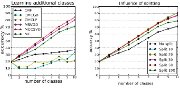
Learning additional classes Influence of splitting

Fig. 5. Left: Results of incremental learning on “pendigits” . The experiment starts with samples from two classes and adds all samples from the next class in every round.Right:Experiments on the same data with varying thresholds✓s to split nodes with uniform class labels (“un-pausing”). Performance is substantially increased using these artificial splits.

all samples from the next class for re-training. This can be seen as the worst case scenario, and it is reflected by the bad performance of the standard online learning methods (see Fig. 5, left). Only the Mondrian forests can handle this hard case comparably well.

C. Benefit of Mondrian block unpausing

As mentioned in Sec. IV-B, we modify the original Mon-drian forest algorithm in an important detail by artificially adding splits in nodes that consist only of samples with the same class label. To show the benefit of this, we plot the results for different values of the splitting threshold ✓s in

Fig. 5 (right). We see that the earlier we decide to split these nodes, the better is the result. We note however that there is a trade-off with the depth of the trees, which leads to higher memory and run-time requirements. In practice, a value of ✓s = 20 has proven to be a good compromise

between efficiency and classification performance.

D. Under- and overconfidence

To evaluate under- or overconfidence of Mondrian forests we generated confidence histograms for correctly and incor-rectly classified samples on a test set from the KITTI set (see Fig. 6). From the histograms in the first row, we see that in the beginning, when only few training samples are available (250 in our case), the ORF is much more overconfident than the MF, while underconfidence is not much different. In numbers we obtained overconfidences of0.415vs.0.820for the MF and the ORF respectively and0.157vs.0.116for the respective underconfidences. This difference is smaller later, when the training set consists of16,000samples (see bottom row in the figure). Here, the numbers are 0.529 and0.583

for overconfidence and0.126and0.132for underconfidence

of MF and ORF. However, for good classification results it is more important to reduce overconfidence already for small training sets, because then the samples that are incorrectly classified but detected as such have a stronger influence and can server better to improve the learned model.

E. Pool-based vs. stream-based Active Learning

In the last set of experiments, we evaluated the perfor-mance of the MF algorithm for the stream-based scenario.

KITTI dataset - Active Learning

Fig. 7. Left:Learning curves of the Mondrian forest for the “re-sample” experiment from Sec. III-C. The MF classifier can deal much better with the data stream.Right:Classification accuracies for Active Learning using an MF and an ORF, where only5%,10%and20%of the most uncertain data points are queried. Again, the MF clearly outperform the standard ORF.

First, we ran the same experiment as described in Sec. III-C, and the result is given in Fig. 7 (left). We can see that the MF classifier increases its classification accuracy much faster than the ORF, even in the stream-based setting, and it also reaches a higher level (about 90% accuracy). We then tested the Active Learning scenario, where new label queries were generated after every 1,000 data samples. From these, we only used the most uncertain predictions for querying and re-training, and this fraction varied between 5% and 20%, i.e. from 50 to 200 samples per learning epoch. The result is shown in the right plot of Fig.7. The plot clearly shows that the MF can improve its classification accuracy even when trained only on a very small fraction of the data. Thus, on one side the MF classifier provides a higher level of learning autonomy by generating less queries and on the other side it can deal with the hard problem of learning from data streams. This is also reflected by the qualitative results in Fig. 8.

VI. CONCLUSIONS

In robotics, stream-based learning applications are much more relevant than standard pool-based approaches, because robots need to be adaptive to new environments. Data streams are however much harder to learn from, but we present a very effective and efficient approach to handle such situations. Based on a recent online learning algorithm, we show that Active Learning can be performed successfully on streams of data. While in our experiments we considered the problem to learn class labels, our approach is also useful for many other applications where semantic information must be au-tomatically inferred from input data streams.

Acknowledgment: This work was funded by the EU project SPENCER (ICT-2011-600877).

REFERENCES

[1] P. Lamon, C. Stachniss, R. Triebel, P. Pfaff, C. Plagemann, G. Grisetti, S. Kolski, W. Burgard, and R. Siegwart, “Mapping with an autonomous car,” in IEEE/RSJ IROS Workshop: Safe Navigation in Open and Dynamic Environments, 2006.

[2] H. Grimmett, R. Paul, R. Triebel, and I. Posner, “Knowing when we don’t know: Introspective classification for mission-critical decision making,” inInt. Conf. on Rob. and Autom. (ICRA), 2013.

[3] T. R¨uhr, J. Sturm, D. Pangercic, M. Beetz, and D. Cremers, “A generalized framework for opening doors and drawers in kitchen environments,” inInt. Conf. on Rob. and Autom. (ICRA), 2012. [4] C. Sammut and G. I. Webb,Encyclopedia of Machine Learning, 2010.

(a) MF - 250 - correct (b) MF - 250 - false (c) ORF - 250 - correct (d) ORF - 250 - false

(e) MF - 16000 - correct (f) MF - 16000 - false (g) ORF - 16000 - correct (h) ORF - 16000 - false

Fig. 6. Confidence values of a Mondrian forest (a, b, e, f) and an online Random Forest (c, d, g, h) on the KITTI data set. The upper row shows the confidence histograms after training on 250 samples and the lower row results after learning on 16,000 samples. We see that the MF is less overconfident, particularly in the beginning with little training data, as it makes wrong predictions with lower confidence (or, equivalently with higher uncertainty). At the same time, it is not more underconfident, as the correct predictions are mostly made with high confidence.

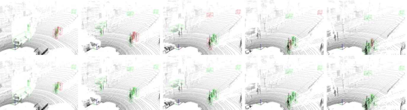
Fig. 8. Further results on the scene given in Fig. 1. From left to right, we show the next five data frames (point clouds), again after training on a stream of 10000 samples. The upper row shows the result for ORF, the lower row the MF result. Again, most classifications are done correctly by the MF (green boxes), while the ORF has many false classifications (red boxes).

[5] V. Polikar, Robi and Upda, Lalita and Upda, Satish S and Honavar, “Learn++: An incremental learning algorithm for supervised neural networks,”Systems, Man, and Cybernetics, Part C: Applications and Reviews, IEEE Transactions on, vol. 31, pp. 497–508, 2001. [6] M. Ristin, M. Guillaumin, J. Gall, and L. V. Gool, “Incremental

Learning of NCM Forests for Large-Scale Image Classification,” Computer Vision and Pattern Recogn. (CVPR), pp. 3654–3661, 2014. [7] T. Mensink, J. Verbeek, F. Perronnin, and G. Csurka,Advanced Topics in Computer Vision, ser. Adv. in Computer Vision and Pattern Recogn., G. M. Farinella, S. Battiato, and R. Cipolla, Eds. Springer, 2013. [8] L. Yang, W.-m. Ma, and B. Tian,Advances in Neural Networks, ser.

LNCS. Springer, 2011, vol. 6676, ch. New Multi-class Classification Method Based on the SVDD Model, pp. 103–112.

[9] A. K. N. Ho, N. Ragot, J. Y. Ramel, V. Eglin, and N. Sidere, “Document classification in a non-stationary environment: A one-class svm approach,” in Proc. of the Intern. Conf. on Document Analysis and Recognition (ICDAR), 2013, pp. 616–620.

[10] A. Saffari, M. Godec, T. Pock, C. Leistner, and H. Bischof, “Online multi-class lpboost,” inCVPR, 2010.

[11] A. Saffari, C. Leistner, J. Santner, M. Godec, and H. Bischof, “On-line random forests,”Computer Vision Workshops (ICCV Workshops), pp. 1393–1400, 2009.

[12] B. Settles,Active Learning. Morgan & Claypool, 2012.

[13] A. Kapoor, K. Grauman, R. Urtasun, and T. Darrell, “Gaussian processes for object categorization,” Intern. Journal of Computer

Vision, vol. 88, no. 2, pp. 169–188, 2010.

[14] A. Vezhnevets, J. Buhmann, and V. Ferrari, “Active learning for semantic segmentation with expected change,” inCVPR, 2012. [15] D. Wang, C. Yan, S. Shan, and X. Chen, “Active learning for

interactive segmentation with expected confidence change,” inAsian Conf. on Computer Vision, 2012.

[16] L. Geurts, Pierre and Ernst, Damien and Wehenkel, “Extremely randomized trees,”Machine learning, vol. 62, pp. 3–42, 2006. [17] A. Geiger, P. Lenz, and R. Urtasun, “Are we ready for autonomous

driving? the KITTI vision benchmark suite,” in Proc. of Conf. on Computer Vision and Pattern Recognition (CVPR), 2012.

[18] B. Lakshminarayanan, D. M. Roy, and Y. W. Teh, “Mondrian Forests: Efficient Online Random Forests,” inAdvances in Neural Information Processing Systems (NIPS), 2014.

[19] D. Mund, R. Triebel, and D. Cremers, “Active online confidence boosting for efficient object classification,” inProc. IEEE Int. Conf. on Robotics and Automation (ICRA), 2015.

[20] E. Alpaydin and C. Kaynak, “Optical Recognition of Handwritten Digits Data Set,” 1995.

[21] H. Himmelsbach, M. and Luettel, T. and Wuensche, “Real-time Object Classification in 3D Point Clouds Using Point Feature Histograms,” inIntern. Conf. on Intell. Robots and Systems (IROS), 2009. [22] L. Bo, X. Ren, and D. Fox, “Hierarchical matching pursuit for image

classification: Architecture and fast algorithms,” inAdvances in neural information processing systems (NIPS), 2011, pp. 2115–2123.