Towards Universal Object Detection

(1)

UC San Diego

UC San Diego Electronic Theses and Dissertations

Permalink https://escholarship.org/uc/item/5v3112g6 Author Cai, Zhaowei Publication Date 2019 Peer reviewed|Thesis/dissertation

(2)

UNIVERSITY OF CALIFORNIA SAN DIEGO

A dissertation submitted in partial satisfaction of the requirements for the degree

Doctor of Philosophy in

Electrical Engineering (Signal and Image Processing) by

Zhaowei Cai

Committee in charge:

Professor Nuno Vasconcelos, Chair Professor Kenneth Kreutz-Delgado Professor David Kriegman

Professor Truong Nguyen Professor Zhuowen Tu

(3)

(4)

The dissertation of Zhaowei Cai is approved, and it is accept-able in quality and form for publication on microfilm and electronically:

Chair

University of California San Diego

(5)

DEDICATION

(6)

EPIGRAPH

Look deep into nature, and then you will understand everything better.

(7)

TABLE OF CONTENTS

Signature Page . . . iii

Dedication . . . iv

Epigraph . . . v

Table of Contents . . . vi

List of Figures . . . x

List of Tables . . . xii

Acknowledgements . . . xiv

Vita . . . xvii

Abstract of the Dissertation . . . xviii

Chapter 1 Introduction . . . 1

1.1 Object Detection . . . 3

1.2 Challenges on Object Detection Universality . . . 3

1.3 Contributions of the Thesis . . . 6

1.3.1 An Efficient Framework for Multi-Scale Detection . . . 6

1.3.2 An Effective Architecture for High-Quality Detection . . . . 7

1.3.3 A Novel Design for Domain-Universal Detection . . . 8

1.3.4 Optimal Detector Solutions under Complexity Constraint . . 8

1.4 Organization of the Thesis . . . 10

Chapter 2 Multi-Scale Object Detection . . . 11

2.1 Introduction . . . 12

2.2 Related Work . . . 14

2.3 Multi-Scale Object Proposal Network . . . 15

2.3.1 Multi-Scale Detection Strategies . . . 16

2.3.2 Architecture . . . 17

2.3.3 Sampling . . . 19

2.3.4 Implementation Details . . . 20

2.4 Object Detection Network . . . 21

2.4.1 CNN Feature Map Approximation . . . 22

2.4.2 Context Embedding . . . 23

2.5 Experimental Evaluation . . . 24

(8)

2.5.2 Object Detection Evaluation . . . 27

2.6 Conclusions . . . 30

2.7 Acknowledgements . . . 30

Chapter 3 High-Quality Object Detection . . . 31

3.3 Review of High-Quality Object Detection . . . 40

3.3.1 Object Detection . . . 40

3.3.2 Detection Quality . . . 42

3.3.3 Challenges to High Quality Detection . . . 43

3.4 Cascade R-CNN . . . 45

3.4.1 Architecture . . . 45

3.4.2 Cascaded Bounding Box Regression . . . 45

3.4.3 Cascaded Detection . . . 46

3.4.4 Differences from Previous Works . . . 48

3.5 Instance Segmentation . . . 50 3.5.1 Mask R-CNN . . . 50 3.5.2 Cascade Mask R-CNN . . . 50 3.6 Experimental Results . . . 52 3.6.1 Experimental Set-up . . . 52 3.6.2 Quality Mismatch . . . 54

3.6.3 Comparison withIterative BBoxandIntegral Loss . . . 56

3.6.4 Ablation Experiments . . . 58

3.6.5 Comparison with the state-of-the-art . . . 60

3.6.6 Generalization Capacity . . . 63

3.6.7 Proposal Evaluation . . . 65

3.6.8 Instance Segmentation by Cascade Mask R-CNN . . . 65

3.6.9 Results on PASCAL VOC . . . 66

3.6.10 Additional Results on other Datasets . . . 68

3.7 Conclusion . . . 70

Chapter 4 Domain-Universal Object Detection . . . 72

4.3 Multi-Domain Object Detection . . . 78

4.3.1 Universal Object Detection Benchmark . . . 78

4.3.2 Single-Domain Detector Bank . . . 79

4.3.3 Adaptive Multi-Domain Detector . . . 79

4.3.4 SE Adapters . . . 81

4.4 Domain-Universal Detection by Domain Attention . . . 82

(9)

4.4.2 Domain-Attentive Universal Detector . . . 83

4.4.3 Universal SE Adapter Bank . . . 84

4.4.4 Domain Attention . . . 85

4.5 Experiments . . . 86

4.5.1 Datasets and Evaluation . . . 87

4.5.2 Single-Domain Detection . . . 87

4.5.3 Multi-Domain Detection . . . 88

4.5.4 Effect of the number of SE adapters . . . 89

4.5.5 Results on the full benchmark . . . 91

4.5.6 Official Evaluation . . . 93

Chapter 5 Learning Complexity-Aware Cascades . . . 97

5.1 Introduction . . . 98 5.2 Related Work . . . 101 5.3 Complexity-Aware Cascade . . . 104 5.3.1 AdaBoost . . . 104 5.3.2 Complexity-Aware Learning . . . 105 5.3.3 Embedded Cascade . . . 107 5.3.4 Cascade Boosting . . . 107 5.3.5 Properties . . . 110 5.3.6 Complexity Loss . . . 112 5.3.7 Weak Learners . . . 113

5.3.8 Bootstrapping and Thresholds . . . 116

5.4 Pedestrian Detector Design . . . 117

5.4.1 Heterogeneous Features . . . 117

5.4.2 Feature Complexity . . . 120

5.4.3 Embedding Large CNN Models . . . 122

5.5 Experiments . . . 125

5.5.1 Experimental Setting . . . 125

5.5.2 Homogeneous Cascade Comparison . . . 126

5.5.3 CompACT Cascade Configuration . . . 127

5.5.4 Benefits of optimal accuracy/complexity trade-off . . . 129

5.5.5 Complexity Restricted vs. Sensitive Trees . . . 131

5.5.6 Embedding Large CNN models . . . 132

5.5.7 Pedestrian Detection on Caltech . . . 135

5.5.8 Pedestrian Detection on KITTI . . . 137

5.5.9 Pedestrian Detection on CityPersons . . . 139

5.5.10 CompACT as Attention Mechanism . . . 139

(10)

Chapter 6 Learning Low-Precision Neural Networks . . . 142 6.1 Introduction . . . 143 6.2 Related Work . . . 145 6.3 Binary Networks . . . 146 6.3.1 Goals . . . 147 6.3.2 Weight Binarization . . . 147

6.3.3 Binary Activation Quantization . . . 148

6.4 Half-wave Gaussian Quantization . . . 149

6.4.1 ReLU . . . 150

6.4.2 Forward Approximation . . . 150

6.4.3 Backward Approximation . . . 153

6.5 Experimental Results . . . 155

6.5.2 Full-precision Activation Comparison . . . 156

6.5.3 Low-bit Activation Quantization Results . . . 157

6.5.4 Backward Approximations Comparison . . . 159

6.5.5 Bit-width Impact . . . 160

6.5.6 Comparison to the state-of-the-art . . . 161

6.5.7 Results on CIFAR-10 . . . 163

Chapter 7 Discussion and Conclusion . . . 165

(11)

LIST OF FIGURES

Figure 1.1: The difference between object classification and object detection. . . 2

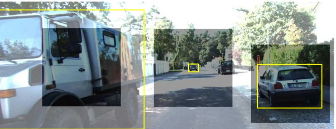
Figure 2.1: In natural images, objects can appear at very different scales, as illustrated

by the yellow bounding boxes. A single receptive field, such as that of the

RPN [140] (shown in the shaded area), cannot match this variability. . . 13

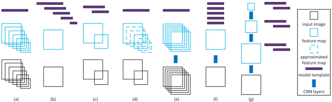
Figure 2.2: Different strategies for multi-scale detection. The length of model template

represents the template size. . . 15

Figure 2.3: Proposal sub-network of the MS-CNN. The bold cubes are the output tensors

of the network. h×wis the filter size, cthe number of classes, andbthe

number of bounding box coordinates. . . 17

Figure 2.4: Object detection sub-network of the MS-CNN. “trunk CNN layers” are

shared with proposal sub-network.W andH are the width and height of the

input image. The green (blue) cubes represent object (context) region pooling. 21

Figure 2.5: Proposal recall on the KITTI validation set (moderate). “hXXX” refers to

input images of height “XXX”. “mt” indicates multi-task learning of proposal

and detection sub-networks. . . 25

Figure 2.6: Proposal performance comparison on KITTI validation set (moderate). The

first row is proposal recall curves and the second row is recall v.s. IoU for

100 proposals. . . 26

Figure 2.7: Comparison to the state-of-the-art on KITTI benchmark test set (moderate). 28

Figure 2.8: Comparison to the state-of-the-art on Caltech. . . 30

Figure 3.1: (a) and (b) detections by object detectors of increasing qualities, and (c)

examples of increasing quality. . . 33

Figure 3.2: Bounding box localization, classification loss and detection performance of

object detectors of increasing IoU thresholdu. . . 34

Figure 3.3: The architectures of different frameworks. “I” is input image, “conv”

back-bone convolutions, “pool” region-wise feature extraction, “H” network head, “B” bounding box, and “C” classification. “B0” is proposals in all architectures. 39

Figure 3.4: IoU histograms of training samples of each cascade stage. The distribution of

the 1st stage is the RPN output. Shown in red are the percentage of positives

for the corresponding IoU threshold. . . 44

Figure 3.5: Distribution of the distance vector ∆ of (3.4) (without normalization) at

different cascade stages. Top: plot of(δx,δy). Bottom: plot of(δw,δh). Red

dots are outliers for the increasing IoU thresholds of later stages, and the

statistics shown are obtained after outlier removal. . . 47

Figure 3.6: Architectures of the Mask R-CNN (a) and three Cascade Mask R-CNN

strategies for instance segmentation (b)-(d). Beyond the definitions of Figure 3.3, “S” denotes a segmentation branch. Note that segmentations branches do not necessarily share heads with the detection branch. . . 51

(12)

Figure 3.7: (a) detection performance of individually trained detectors, with their own proposals (solid curves) or Cascade R-CNN stage proposals (dashed curves).

(b) results of adding ground truth to the proposal set. . . 55

Figure 3.8: Detection performance of all Cascade R-CNN detectors at all cascade stages. 56 Figure 3.9: (a) localization performance ofiterative BBoxand Cascade R-CNN regres-sors. (b) detection performance of the individual classifiers of theintegral lossdetector. . . 57

Figure 4.1: Samples of our universal object detection benchmark. . . 74

Figure 4.2: Multi-domain and universal object detectors for three domains. “D” is the domain, “O” the output, “A” domain-specific adapter, and “DA” the proposed domain attention module. The blue color and the DA are domain-universal, but the other colors domain-specific. . . 75

Figure 4.3: The activation statistics of all single-domain detectors. . . 80

Figure 4.4: (a) block diagram of SE adapter and (b) SE adapter bank. . . 81

Figure 4.5: The block diagram (top) and the detailed view (down) of the proposed domain adaptation module. . . 83

Figure 4.6: Soft assignments across SE units for all datasets. . . 91

Figure 5.1: Decision tree of depth 2. Circles represent classifier nodes, squares terminal nodes. φ(x,v)is the feature ofxused at nodev,θa threshold. . . 113

Figure 5.2: Sample of the feature channels generated on a pedestrian image. . . 117

Figure 5.3: Eight 2×2 checkerboard-like filters used in this work. Red (Green) is used to represent value +1 (-1). . . 119

Figure 5.4: CNN architecture used to extract small CNN features. . . 120

Figure 5.5: Cascade accuracy v.s. complexity for different features. . . 126

Figure 5.6: Stage configuration learned with different trade-off coefficientη. Only one in five stages is shown. . . 127

Figure 5.7: Accuracy v.s. complexity for different trade-off coefficientsη. . . 128

Figure 5.8: Stage configuration for “Boosting” and “Manual” cascades. . . 130

Figure 5.9: Comparison to the state-of-the-art on Caltech (reasonable). . . 136

Figure 5.10: Processing time spent per Caltech test image. . . 139

Figure 6.1: Forward and backward functions for binarysign(left) and half-wave Gaus-sian quantization (right) activations. . . 148

Figure 6.2: Dot-product distributions on different layers of AlexNet with binary weights and quantized activations (100 random images). . . 152

Figure 6.3: Backward piece-wise activation functions of clipped ReLU and log-tailed ReLU. . . 154

Figure 6.4: The error curves of training (thin) and test (thick) for sign(x) and Q(x) (HWGQ) activation functions. . . 158

Figure 6.5: The error curves of training (thin) and test (thick) for alternative backward approximations. . . 159

(13)

LIST OF TABLES

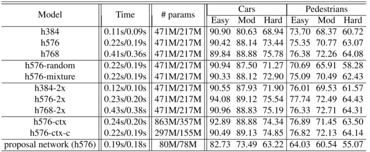
Table 2.1: Parameter configurations of the different models. . . 24

Table 2.2: Detection recall of the various detection layers on KITTI validation set (car), as a function of object hight in pixels. . . 25

Table 2.3: Results on the KITTI validation set. “hXXX” indicates an input of height “XXX”, “2x” deconvolution, “ctx” context encoding, and “c” dimensionality reduction convolution. In columns “Time” and “# params”, entries before the “/” are for car model and after for pedestrian/cyclist model. . . 27

Table 2.4: Results on the KITTI benchmark test set (only published works shown). . . 29

Table 3.1: Comparison of the Cascade R-CNN with iterative BBox and integral loss detectors. . . 57

Table 3.2: Stagewise performance of the Cascade R-CNN. 1∼3 indicates an ensemble result, obtained by averaging the three classifier probabilities for 3rd stage proposals. . . 58

Table 3.3: Ablation experiments. “IoU↑” indicates increasing IoU thresholds, “update statistics” updating regression statistics, and “stage loss” weighting of stage losses. . . 59

Table 3.4: The impact of the number of stages in Cascade R-CNN. . . 60

Table 3.5: Performance of state-of-the-artsingle-modeldetectors on COCOtest-dev. Entries denoted by∗and?use enhancements at training and inference, respec-tively. . . 61

Table 3.6: Performance of Cascade R-CNN implementations with multiple detectors. All speeds are reported per image on a single Titan Xp GPU. . . 62

Table 3.7: Performance of various implementations of the Cascade R-CNN with the FPN detector on Detectron, using the1xschedule. . . 64

Table 3.8: Proposal recall of Cascade R-CNN stages. . . 65

Table 3.9: The instance segmentation comparison among three strategies of the Cascade Mask R-CNN. . . 66

Table 3.10: Performance of the Cascade Mask R-CNN on multiple backbone networks on COCO 2017val. ∗and?denotes enhancement techniques at training and inference, respectively, as in [49]. . . 67

Table 3.11: Detection results on PASCAL VOC 2007test. . . 68

Table 3.12: MS-CNN detection results for the car class on KITTI test set. . . 69

Table 3.13: MS-CNN detection results on CityPersons validation set. . . 69

Table 3.14: MS-CNN Detection results on WiderFace validation set. . . 70

Table 4.1: The dataset details, the domain-specific hyperparameters and the performance of the single-domain detectors. “T/V/T” means train/val/test, “size” the shortest side of inputs,BS RPN batch size, andS/R anchor “scales/aspect ratios”. . . 86

(14)

Table 4.2: The comparison on multi-domain detection. † denotes fixed assignment. “time” is the relatively run-times on the five datasets when the domain is

unknown. . . 88

Table 4.3: The effect of SE adapters number. . . 88

Table 4.4: Overall results on the full universal object detection benchmark (11 datasets). “ada” indicates adapter, “WF” WiderFace, “DL” DeepLesion, “WC” Watercolor. 90 Table 4.5: The comparison on VOC 2007test. ‡/† denotes with COCOtrainval/val 93 Table 4.6: The comparison on WiderFaceVal. . . 93

Table 4.7: The comparison on KITTItestset of car. . . 94

Table 4.8: Sensitivity at 4 FPs per image on DeepLesiontestset. . . 94

Table 4.9: The comparison on Clipart, Watercolor and Comictestset. . . 95

Table 5.1: Feature complexity and processing unit . . . 121

Table 5.2: Comparison to “Boosting” and “Manual” cascades. . . 131

Table 5.3: Comparison of complexity restricted and sensitive trees. . . 131

Table 5.4: Faster-RCNN baseline results. . . 132

Table 5.5: Embedding of large CNNs in CompACT cascades. “+” denotes additional time, after embedding the CNN, over CompACT. . . 133

Table 5.6: Pedestrian detection mAP comparison on KITTI. . . 137

Table 5.7: The results on CityPersons validation set. . . 138

Table 6.1: Full-precision Activation Comparison for AlexNet. . . 157

Table 6.2: Low-bit Activation Comparison. . . 157

Table 6.3: Backward Approximations Comparison. . . 159

Table 6.4: Bit-width Comparison of Activation Quantization. . . 160

Table 6.5: HWGQ implementation of various popular networks. . . 161

Table 6.6: Comparison to state-of-the-art low-precision methods. Top-1 gap to the corresponding full-precision network is also reported. . . 162

Table 6.7: The results on CIFAR-10. The bit width before and after “+” is for weights and activations respectively. . . 163

(15)

ACKNOWLEDGEMENTS

Finishing the PhD degree would be impossible for me, without the help, support, discus-sion, and company from many people. I would like to express my sincere gratitude to my family, advisor, thesis committee members, mentors, collaborators, colleagues, friends, etc.

At first, I would like to thank my PhD advisor, Professor Nuno Vasconcelos. It was my great honor to work under his supervision. His critical thinking, research philosophy, technical writing/presentation, etc., have reshaped my research mindset. I would also like to thank Profes-sors Kenneth Kreutz-Delgado, David Kriegman, Truong Nguyen, and Zhuowen Tu for being my committee members and their insightful suggestions and comments.

I was fortunate to work as a research intern in multiple industry research labs. Those research experiences are insightful and unique. I would like to thank Dr. Quanfu Fan and Rogerio Feris of IBM Watson Research, for offering me my first industry research intern experience and their support and help for my project. I would also like to thanks Dr. Xiaodong He and Jian Sun for being my mentors at Microsoft Research. In addition, I am also greatly appreciated to work with Dr. Kaiming He, Ross Girshick and Piotr Dollar at Facebook AI Research. They are the people I look up to in the research area of object detection. Their vision and rigorous experimental validation have deep effect on me as a researcher.

I would like to thank my undergraduate advisor, professor Qi Zhang, for introducing me into this fantastic field of computer vision in the first place, and my career path has been completely changed. I also want to thank my intern advisors, Stan Z. Li, Zhen Lei, Dong Yi, and Shengcai Liao, for providing a rigorous academic training to me at Institute of Automation, Chinese Academy of Science. And my gratitude also goes to my close collaborator, Longyin Wen, for those countless hours of working together.

I also want to thank my colleagues of SVCL who have overlap with me, Dashan Gao, Mohammad Saberian, Jose Costa Pereira, Weixin Li, Mandar Dixit, Can Xu, Song Lu, Si Chen, Bo Liu, Yingwei Li, Pedro Morgado, Yi Li, Pei Wang, John Ho, Gina Wu, Brandon Leung,

(16)

Xudong Wang, Gautam Nain, Yang Du, Xiangyun Zhao, Xin Dong, etc. Without their company, the research and life during my PhD study will be much more difficult. Among them, I am particularly thankful to Mohammad Saberian who was very helpful when I started to work at SVCL on object detection, Dashan Gao and Xudong Wang who are co-authors with me, and Jose Costa Pereira, Yingwei Li and Pedro Morgado for maintaining the servers at the lab. I would like to thank also my friends I met at UCSD, Saining Xie, Eshed Ohn-Bar, Yongxi Lu, Yufei Wang, Panqu Wang, Ning Ma, Mengting Wan, Xiaochu Liu, Tong Jiang, Xueying Lyu, Chicheng Zhang, Lidaling Yi, Yundi Zheng, Jiahao Gong and many others, for bringing laughs, happiness and diversity into my life and study.

Outside of UCSD, I am fortunate to meet many friends, who have broaden my horizons, including Xinlei Chen, Haoqi Fan, Chuang Gan, Zhe Gan, Wenbo Li, Sifei Liu, Jiasen Lu, Xi Peng, Joshua San Miguel, Shenlong Wang, Xiaolong Wang, Fan Wei, Yuxin Wu, Cihang Xie, Junjie Yan, Jianwei Yang, Zhengheng Yang, Xi Yin, Licheng Yu, Zhiwei Zhang, Ziyu Zhang, Yuyin Zhou, Bohan Zhuang, and many others.

Finally, and most importantly, I would like to thank my family. I am very grateful that my parents were fully supportive that I pursue my PhD degree. I also owe my grandparents gratitude, who were my guardians when I was a child. I also want to thank my younger brother, who is the company of my family when I am thousands of miles away home. I am deeply thank for their unconditional love and support.

Chapter 2 is, in full, based on the material as it appears in the publication of “A Unified Multi-scale Deep Convolutional Neural Network for Fast Object Detection”, Zhaowei Cai, Quanfu

Fan, Rogerio Feris, and Nuno Vasconcelos, InProceedings of 14th European Conference on

Computer Vision(ECCV), 2016. The dissertation author was the primary investigator and author of this material.

Chapter 3 is, in full, based on the material as it appears in the publication of “Cascade R-CNN: High Quality Object Detection and Instance Segmentation”, Zhaowei Cai, and Nuno

(17)

Vasconcelos, to appear at IEEE Transactions on Pattern Analysis and Machine Intelligence

(TPAMI), 2020. The dissertation author was the primary investigator and author of this material. Chapter 4 is, in full, based on the material as it appears in the publication of “Towards Universal Object Detection by Domain Attention”, Xudong Wang, Zhaowei Cai, Dashan Gao,

and Nuno Vasconcelos, In Proceedings of IEEE Conference on Computer Vision and Pattern

Recognition(CVPR), 2019. The dissertation author was a joint primary investigator and author of this material.

Chapter 5 is, in full, based on the material as it appears in the publication of “Learning Complexity-Aware Cascades for Pedestrian Detection”, Zhaowei Cai, Mohammad Saberian, and

Nuno Vasconcelos, to appear atIEEE Transactions on Pattern Analysis and Machine Intelligence

(TPAMI), 2019. The dissertation author was the primary investigator and author of this material. Chapter 6 is, in full, based on the material as it appears in the publication of “Deep Learning with Low Precision by Half-wave Gaussian Quantization”, Zhaowei Cai, Xiaodong

He, Jian Sun, and Nuno Vasconcelos, InProceedings of IEEE Conference on Computer Vision

and Pattern Recognition(CVPR), 2017. The dissertation author was the primary investigator and author of this material.

(18)

VITA

2011 B. S. in Automation, Dalian Maritime University, China

2019 M. S. in Electrical Engineering (Signal and Image Processing), University

of California San Diego, United States

2019 Ph. D. in Electrical Engineering (Signal and Image Processing), University

of California San Diego, United States

PUBLICATIONS

Zhaowei Cai, and Nuno Vasconcelos, “Cascade R-CNN: High Quality Object Detection and

Instance Segmentation”, to appear at IEEE Transactions on Pattern Analysis and Machine

Intelligence(TPAMI), 2020.

Zhaowei Cai, Mohammad Saberian, and Nuno Vasconcelos, “Learning Complexity-Aware

Cascades for Pedestrian Detection”, to appear at IEEE Transactions on Pattern Analysis and

Machine Intelligence(TPAMI), 2019.

Xudong Wang,Zhaowei Cai, Dashan Gao, and Nuno Vasconcelos, “Towards Universal Object

Detection by Domain Attention”, InProceedings of IEEE Conference on Computer Vision and

Pattern Recognition(CVPR), 2019.

Zhaowei Cai, and Nuno Vasconcelos, “Cascade R-CNN: Delving into High Quality Object

Detection”, InProceedings of IEEE Conference on Computer Vision and Pattern Recognition

(CVPR), 2018.

Zhaowei Cai, Xiaodong He, Jian Sun, and Nuno Vasconcelos, “Deep Learning with Low

Precision by Half-wave Gaussian Quantization”, InProceedings of IEEE Conference on Computer

Vision and Pattern Recognition(CVPR), 2017.

Zhaowei Cai, Quanfu Fan, Rogerio Feris, and Nuno Vasconcelos, “A Unified Multi-scale Deep

Convolutional Neural Network for Fast Object Detection”, In Proceedings of 14th European

Conference on Computer Vision(ECCV), 2016.

Zhaowei Cai, Mohammad Saberian, and Nuno Vasconcelos, “Learning Complexity-Aware

Cascades for Deep Pedestrian Detection”, InProceedings of IEEE International Conference on

(19)

ABSTRACT OF THE DISSERTATION

by

Zhaowei Cai

Doctor of Philosophy in Electrical Engineering (Signal and Image Processing)

University of California San Diego, 2019

Professor Nuno Vasconcelos, Chair

Object detection is one of the most important and challenging research topics in computer vision. It is playing an important role in our everyday life and has many applications, e.g. surveillance, autonomous driving, robotics, drone, medical imaging, etc. The ultimate goal of object detection is a universal object detector that can work very well in any case under any condition like human vision system. However, there are multiple challenges on the universality of object detection, e.g. scale-variance, high-quality requirement, domain shift, computational constraint, etc. These will prevent the object detector from being widely used for various scales of objects, critical applications requiring extremely accurate localization, scenarios with changing domain priors, and diverse hardware settings. To address these challenges, multiple solutions

(20)

have been proposed in this thesis. These include an efficient multi-scale architecture to achieve scale-invariant detection, a robust multi-stage framework effective for high-quality requirement, a cross-domain solution to extend the universality over various domains, and a design of complexity-aware cascades and a novel low-precision network to enhance the universality under different computational constraints. All these efforts have substantially improved the universality of object detection, and the advanced object detector can be applied to broader environments.

(21)

Chapter 1

Introduction

(22)

boat

person

(a) Object Classification

boat

person

(b) Object Detection

Figure 1.1: The difference between object classification and object detection.

Computer vision is a scientific field that studies the acquisition, extraction, processing, analysis, interpretation and understanding of digital images in order to produce numerical or symbolic information, e.g. in the forms of decisions. This image understanding can be seen as the disentangling of symbolic information from image data using models constructed with the aid of geometry, physics, statistics, and learning theory [111, 39]. It is an interdisciplinary scientific filed with cognitive science, robotics, machine learning, statistics, etc. Its goal is to simulate the human vision system by automatic machines. It has multiple sub-domains, including visual recognition, action understanding, image retrieval, video tracking, segmentation, 3D reconstruction, etc.

Computer vision tasks have achieved great successes in recent years, powered by the recent great successes of deep learning [86, 150, 152, 61]. These are enabled by big data, e.g. large scale annotated dataset, and big computation, e.g. distributed or parallel computations. The feature representation learning by deep neural network is much more representative and powerful than the hand-crafted feature extraction, e.g. HOG [26] and SIFT [109]. The substantial progresses in computer vision make it possible to deploy computer vision algorithms into critical applications, e.g. autonomous driving, medical imaging diagnosis, surgery and service robotics, etc.

(23)

1.1

Object Detection

Object detection is one of the most important and challenging research topics in computer vision. What is object detection? Object classification is probably a more common problem. Given an image, the task is to answer the question of “what”. For example, in Figure 1.1 (a), there are a person and a boat. In addition to the question of “what”, object detection also needs to answer the “where” question. For example, in Figure 1.1 (b), knowing there are a person and a boat is not enough. We also want to where they are.

Object detection is important. On one hand, it has many practical applications, e.g. surveillance, autonomous robot, drone, medical imaging, etc. For example, in autonomous driving, object detection is used to localize objects, understand surrounding environments, and help to make safe decisions. It can also help to detect the lesion in medical CT scans to alleviate the burden of radiologists. On the other hand, object detection is a upstream task in computer vision, supporting many downstream tasks, like visual question answering, captioning, visual navigation, robot grasping, knowledge graph, pose estimation, etc. For example, object detection can not only help the robot arm to accurately grasp the objects in the physical world, but also enable bots to better understand the image semantics and provide more precise answers to the questions asked by the users. Hence, the advancement of object detection is necessary. It will benefit many other sub-domains of computer vision and improve practical computer vision systems to better serve our everyday life.

1.2

Challenges on Object Detection Universality

Despite object detection has made huge progresses in recent years [51, 59, 50, 140, 99, 58], there are still many unresolved challenges. For example, the object detector is usually required to produce accurate detection results of various categories, scales, aspect ratios, etc, and sometimes even with serious lighting changes, occlusion, background distraction, etc. It is very challenging

(24)

to develop a universal object detector that can work well in any case under any condition like human visual system. In specific, the universality challenge has multiple aspects, including scale-variance, high-quality requirement, domain shift, device and computation constraints, etc. First, scale invariance is an important requisite for effective object detection, since the

objects could be presented with huge scale variation, e.g. from 5×5 pixels to 1000×1000 pixels,

in a typical image. A detector should detect all objects without scale bias. This is important for practical application of object detection. For example, in the vision system of autonomous vehicle, where the further objects are usually visually smaller, if smaller (further) objects can be successfully detected, the control system will have more time to respond. However, the detection of small objects is much more difficult than that of large objects, reducing the universality of object detection in scale. There are mainly two reasons responsible for this: 1) the feature extraction is not scale invariant; and 2) it is nontrivial to design an effective and efficient multi-scale detection framework. To address each of them, before the resurgence of deep learning, the solutions are to manually design better feature extraction, e.g. HOG [26] and SIFT [109], and to use the image pyramid strategy, respectively. However, the handcrafted feature extraction is not very representative and the image pyramid is very time-consuming. Although deep neural networks can offer much more powerful feature representations, the design of efficient multi-scale detection system within neural network is not trivial.

Second, detection quality is an important indicator of how good an object detector is. Higher detection quality means the detector can produce detection results that have tighter coverage with the ground truths. The tightness is evaluated by a metric, called intersection over union (IoU), between a detection and the corresponding ground truth. If the IoU is above a threshold, e.g. 0.5, the detection is a success, otherwise, a failure. However, the importance of high-quality detection is generally neglected in the area of object detection. This is partially because the detection evaluation metrics have historically placed greater emphasis on the low-quality detection regime. Many object detection datasets, including the very popular PASCAL

(25)

VOC [36], ImageNet [143], Caltech Pedestrian[32], etc., use IoU threshold of 0.5 in evaluation, which is a very loose requirement. Nevertheless, it is important to have high quality detections, e.g. using IoU threshold of 0.7. For example, if the detection of a pedestrian is not highly accurate, the vision system of an autonomous vehicle could mispredict the pedestrian crossing the street as walking on the sidewalk. Another example is from robotics, e.g. surgery or service robots. Any visual detection in surgery robot is required to be highly precise. Nobody wants his/her organs or tissues to be mislocalized or miscut in any way. The consequences of low quality detection in these critical applications are very serious. The current object detectors are usually good at low-quality detection, but not high-quality detection. It is very challenging to design quality-universal object detection system.

Third, existing detectors are usuallydomain-specific, e.g. trained and tested on a single

dataset, instead of domain-universal. This is partially due to the fact that object detection

datasets are diverse and there are nontrivial domain shifts among them. In general, high detection performance requires a detector specialized on the target dataset. This poses a significant problem for practical applications, which are not usually restricted to any one of the domains. For example, an autonomous robot can go into any environments, with changing illumination, background,

weather, etc. Thedomain-specificdetector probably will fail in this case. Hence, there is a need

for systems capable of detecting objects regardless of the domains. However, developing this domain universal detection system is very challenging, e.g. for more than thousands of different domains, considering that a single model may not have enough capacity to cover the substantial domain shifts and the model size and computation need to be prevented from being increasing too much.

Fourth, object detection is an indispensable module in many computer vision systems, which are frequently required to run on different kinds of hardware. Although the overwhelming popularity of neural networks make the GPU as the most popular hardware, its disadvantages including expensive price, high power usage, large volume, heavy weight, etc., encourage to

(26)

use other hardware to meet different kinds of needs, e.g. CPU, FPGA, cellphone, raspberry pi, etc. However, these non-GPU hardware generally has strong constraints on power, computation, memory, etc., which could be orders of lower than those of GPUs. In these cases, the detector usually has to compromise on speed and performance due to the constraints. Therefore, the current object detectors are not universal for different devices or under different constraints. How to improve speed, reduce power consumption and remain accuracy on non-GPU devices are important and challenging.

1.3

Contributions of the Thesis

In this thesis, we mainly try to tackle the four challenges mentioned above, scale, quality, domain and complexity constraint, and to advance the universality of object detection.

1.3.1

An Efficient Framework for Multi-Scale Detection

Although deep neural networks have achieved great successes in object detection [51, 59, 50, 140, 99, 58], how to design effective and efficient multi-scale detection system in neural networks is still under exploration. Our goal is to develop a new architecture of convolutional neural network for multi-scale object detection, improving the detection universality across scales. The scale-invariant detection is traditionally addressed by operating a scale-specific detector on a pyramid of images: the larger (smaller) objects are detected on the coarser (finer) resolution image. The outputs on all pyramid images are grouped together as the final detection results. However, this strategy is not desirable, especially for neural networks, because it requires to run the expensive network multiple times for all images in the pyramid. Instead, we avoid the problem by resorting to a pyramid of features, as an approximation to image pyramid. The efficient feature pyramid will be achieved by forwarding the original input image to the expensive network only once, and then multiple scale-specific light-weight detectors run on corresponding

(27)

feature scale. These complementary detectors are grouped together as a final strong multi-scale object detector. This feature pyramid strategy can successfully avoid the repetitive expensive network computations for image pyramid, and thus are much more efficient. The experiments have shown that it can significantly improve the detection performance on small objects, enabling better scale-invariant detection. Thus, the universality over scale is advanced.

1.3.2

An Effective Architecture for High-Quality Detection

In object detection, there are many “close” false positives presented in an image, cor-responding to “close but not correct” bounding boxes. An effective detector must find all true positives, while suppressing these close false positives. This requirement makes detection more difficult than object recognition. Unlike the latter, an intersection over union (IoU) threshold is

required to define positives/negatives in object detection, which as well defines itsquality. While

the threshold is typically set at the value of 0.5, this is a very loose requirement for positives. The resulting detectors frequently produce noisy (low quality) detections. However, detection performance usually degrades when using higher training IoU thresholds. This is denoted the

paradoxof high quality detection and has two main causes: 1) overfitting, due to exponentially vanishing positive training sets for large thresholds, and 2) inference-time mismatch between the IoUs for which the detector is optimal and those of the test hypotheses. A multi-stage object detection architecture, the Cascade R-CNN, is proposed to address these problems. It consists of a sequence of detectors trained with increasing IoU thresholds, so that deeper stages are more selective against close false positives. The detectors are trained sequentially, using the output of a detector as the training set for the subsequent one. This resampling operation progressively improves hypotheses quality, guaranteing that all detectors have a positive training set of equiva-lent size and thereby eliminating overfitting problem. The use of the same cascade procedure at inference time then eliminates the quality mismatch between the hypotheses and the detector of each stage. The Cascade R-CNN has been shown to significantly improve the high-quality object

(28)

detection, and thus advance the detection universality over quality.

1.3.3

A Novel Design for Domain-Universal Detection

Despite increasing efforts on multi-domain/universal representations for visual recognition, few have addressed object detection. In this thesis, we developed a few systems for multi-domain and domain-universal object detection, capable of working on various image domains, e.g. from human faces and traffic signs to medical CT images. In the multi-domain system, a new family of domain adapter for object detection was introduced which is effective and efficient, based on the principles of squeeze and excitation. However, this multi-domain detection system still requires domain prior, knowing which domain to work on in advance. Unlike the multi-domain system, the domain-universal system does not require prior knowledge of the domain of interest. This is achieved by the introduction of a new attention mechanism. In this domain-universal system, all parameters and computations are shared across domains, and a single network processes all domains all the time. The experiments have shown that these solutions can substantially extend the detector universality across a large number of domains with small amount of increases in overall model size and computation.

1.3.4

Optimal Detector Solutions under Complexity Constraint

How to improve speeds and reduce power consumption are necessary for object detection. We tried to tackle these challenges from two aspects: the design of a novel complexity-aware detector cascade and learning efficient low-precision networks. They improve the detection universality across computation constraints and hardware.

Cascade object detector is one of the most popular detection frameworks in the history, especially before the resurgence of deep learning. We investigated the design of complexity-aware cascaded detectors, combining features of very different complexities. This cascade procedure is

(29)

designed, by formulating cascade learning as the Lagrangian optimization of a risk that accounts

for both accuracy and complexity. A boosting algorithm, denoted ascomplexity aware cascade

training(CompACT), is then derived to solve this optimization. CompACT cascades are shown to seek an optimal trade-off between accuracy and complexity by pushing features of higher complexity to the later cascade stages, where only a few difficult candidate patches remain to be classified. This enables the use of features of vastly different complexities in a single detector. In result, the feature pool can be expanded to features previously impractical for cascade design, such as the responses of a deep convolutional neural network (CNN). This leads to mixed CPU/GPU solutions, that provide practitioners with flexible families of models, ranging from cheap and energy efficient CPU-based cascades, to cascades using GPU stages that emphasize recognition accuracy. This enables accurate cascade at fairly fast speeds.

Current cutting-edge computer vision systems extensively rely on deep neural networks, which are heavy in terms of computation and memory, and require specialized expensive hard-ware, e.g. GPUs. Substantial speed-ups will be made possible if, both activations and weights of a network are binarized or quantized to low-bit, leveraging the property that the expensive float-point computation of dot-product can be replaced by efficient bit operations. However, this is challenging and suffers from substantial accuracy loss, especially when the activations are quantized. Thus, we investigated the problem of quantizing the activations for the speeds-up of neural networks. In previous binary quantization approaches, this problem consists of approxi-mating a classical non-linearity, the hyperbolic tangent, by two functions: a piecewise constant

signfunction, which is used in feedforward network computations, and a piecewise linearhard

tanhfunction, used in the backpropagation step during network learning. Instead, we considered

to approximate the widely used ReLU non-linearity. An half-wave Gaussian quantizer (HWGQ) is proposed for forward approximation and shown to have efficient implementation, by exploiting the statistics of network activations and batch normalization operations. To overcome the problem of gradient mismatch, due to the use of different forward and backward approximations, several

(30)

piece-wise backward approximators are then investigated. The implementation of the resulting quantized network, denoted as HWGQ-Net, is shown to achieve much closer performance to full precision networks. This network quantization technique can be used to significantly improve the running speeds and save power for object detectors based on deep neural networks, enabling them to run on non-GPU devices, e.g. CPU or FPGA.

1.4

Organization of the Thesis

The rest of the thesis is organized as follows. Chapter 2 describes an efficient and effective architecture of convolutional neural network for multi-scale object detection, which is shown to enable better scale-invariant detection. In Chapter 3, we review the novel multi-stage architecture for high-quality object detection, denoted as Cascade R-CNN, and show that this simple design can achieve very robust and strong high-quality detection. Chapter 4 introduces a few solutions for multi-domain and domain-universal object detection, to improve the detection universality across different domains. Chapter 5 investigates the design of complexity-aware cascaded detectors, combining features of very different complexities. The proposed cascades are shown to seek an optimal trade-off between accuracy and complexity by pushing features of higher complexity to the later cascade stages, where only a few difficult candidate patches remain to be classified. In Chapter 6, we present a new quantization technique for low-precision networks, which can significantly save computation and memory with minor accuracy drop, enabling running expensive neural networks on non-GPU devices, e.g. CPU or FPGA. Finally, the thesis is summarized and concluded in Chapter 7.

(31)

Chapter 2

(32)

2.1

Introduction

Classical object detectors, based on the sliding window paradigm, search for objects at multiple scales and aspect ratios. While real-time detectors are available for certain classes of objects, e.g. faces or pedestrians [161, 29], it has proven difficult to build detectors of multiple object classes under this paradigm. Recently, there has been interest in detectors derived from deep convolutional neural networks (CNNs) [51, 50, 16, 59, 46]. While these have shown much greater ability to address the multiclass problem, less progress has been made towards the detection of objects at multiple scales. The R-CNN [51] samples object proposals at multiple scales, using

a preliminary attention stage [158], and then warps these proposals to the size (e.g. 224×224)

supported by the CNN. This is, however, very inefficient from a computational standpoint. The development of an effective and computationally efficient region proposal mechanism is still an open problem. The more recent Faster-RCNN [140] addresses the issue with a region proposal network (RPN), which enables end-to-end training. However, the RPN generates proposals of multiple scales by sliding a fixed set of filters over a fixed set of convolutional feature maps. This creates an inconsistency between the sizes of objects, which are variable, and filter receptive fields, which are fixed. As shown in Figure 2.1, a fixed receptive field cannot cover the multiple scales at which objects appear in natural scenes. This compromises detection performance, which tends to be particularly poor for small objects, like that in the center of Figure 2.1. In fact, [50, 16, 140] handle such objects by upsampling the input image both at training and testing time. This increases the memory and computation costs of the detector.

This work proposes a unified multi-scale deep CNN, denoted themulti-scale CNN

(MS-CNN), for fast object detection. Similar to [140], this network consists of two sub-networks: an object proposal network and an accurate detection network. Both of them are learned end-to-end and share computations. However, to ease the inconsistency between the sizes of objects and receptive fields, object detection is performed with multiple output layers, each focusing

(33)

Figure 2.1: In natural images, objects can appear at very different scales, as illustrated by the yellow bounding boxes. A single receptive field, such as that of the RPN [140] (shown in the shaded area), cannot match this variability.

on objects within certain scale ranges (see Figure 2.3). The intuition is that lower network layers, such as “conv-3,” have smaller receptive fields, better matched to detect small objects. Conversely, higher layers, such as “conv-5,” are best suited for the detection of large objects. The complimentary detectors at different output layers are combined to form a strong multi-scale detector. This is shown to produce accurate object proposals on detection benchmarks with large variation of scale, such as KITTI [43], achieving a recall of over 95% for only 100 proposals.

A second contribution of this work is the use of feature upsampling as an alternative to input upsampling. This is achieved by introducing a deconvolutional layer that increases the resolution of feature maps (see Figure 2.4), enabling small objects to produce larger regions of strong response. This is shown to reduce memory and computation costs. While deconvolution has been explored for segmentation [107] and edge detection [173], it is, as far as we know, for the first time used to speed up and improve detection. When combined with efficient context encoding and hard negative mining, it results in a detector that advances the state-of-the-art detection on the KITTI [43] and Caltech [32] benchmarks. Without image upsampling, the MS-CNN achieves

(34)

2.2

Related Work

One of the earliest methods to achieve real-time detection with high accuracy was the cascaded detector of [161]. This architecture has been widely used to implement sliding window detectors for faces [161, 8], pedestrians [29, 11] and cars [122]. Two main streams of research have been pursued to improve its speed: fast feature extraction [161, 29] and cascade learning [8, 145, 11]. In [161], a set of efficient Haar features was proposed with recourse to integral images. The aggregate feature channels (ACF) of [29] made it possible to compute HOG features at about 100 fps. On the learning front, [8] proposed the soft-cascade, a method to transform a classifier learned with boosting into a cascade with certain guarantees in terms of false positive and detection rate. [145] introduced a Lagrangian formulation to learn cascades that achieve the optimal trade-off between accuracy and computational complexity. [11] extended this formulation for cascades of highly heterogeneous features, ranging from ACF set to deep CNNs, with widely different complexity. The main current limitation of detector cascades is the difficulty of implementing multiclass detectors under this architecture.

In an attempt to leverage the success of deep neural networks for object classification, [51] proposed the R-CNN detector. This combines an object proposal mechanism [158] and a CNN classifier [86]. While the R-CNN surpassed previous detectors [38, 164] by a large margin, its speed is limited by the need for object proposal generation and repeated CNN evaluation. [59] has shown that this could be ameliorated with recourse to spatial pyramid pooling (SPP), which allows the computation of CNN features once per image, increasing the detection speed by an order of magnitude. Building on SPP, the Fast-RCNN [50] introduced the ideas of back-propagation through the ROI pooling layer and multi-task learning of a classifier and a bounding box regressor. However, it still depends on bottom-up proposal generation. More recently, the Faster-RCNN [140] has addressed the generation of object proposals and classifier within a single neural network, leading to a significant speedup for proposal detection. Another interesting work

(35)

(a) (b) (c) (d) (e) (f) (g) input image feature map model template CNN layers approximated feature map

Figure 2.2: Different strategies for multi-scale detection. The length of model template

repre-sents the template size.

is YOLO [137], which outputs object detections within a 7×7 grid. This network runs at∼40 fps,

but with some compromise of detection accuracy.

For object recognition, it has been shown beneficial to combine multiple losses, defined on intermediate layers of a single network [152, 88, 107, 173]. GoogLeNet [152] proposed the use of three weighted classification losses, applied at layers of intermediate heights, showing that this type of regularization is useful for very deep models. The deeply supervised network architecture of [88] extended this idea to a larger number of layers. The fact that higher layers convey more semantic information motivated [107] to combine features from intermediate layers, leading to more accurate semantic segmentation. A similar idea was shown useful for edge detection in [173]. Similar to [152, 88, 107, 173], the proposed MS-CNN is learned with losses that account for intermediate layer outputs. However, the aim is not to simply regularize the learning, as in [152, 88], or provide detailed information for higher outputs, as in [107, 173]. Instead, the goal is to produce a strong individual object detector at each intermediate output layer.

2.3

Multi-Scale Object Proposal Network

(36)

2.3.1

Multi-Scale Detection Strategies

The coverage of many object scales is a critical problem for object detection. Since a detector is basically a dot-product between a learned template and an image region, the template has to be matched to the spatial support of the object to recognize. There are two main strategies to achieve this goal. The first is to learn a single classifier and rescale the image multiple times, so that the classifier can match all possible object sizes. As illustrated in Figure 2.2 (a), this strategy requires feature computation at multiple image scales. While it usually produces the most accurate detection, it tends to be very costly. An alternative approach is to apply multiple classifiers to a single input image. This strategy, illustrated in Figure 2.2 (b), avoids the repeated computation of feature maps and tends to be efficient. However, it requires an individual classifier for each object scale and usually fails to produce good detectors. Several approaches have been proposed to achieve a good trade-off between accuracy and complexity. For example, the strategy of Figure 2.2 (c) is to rescale the input a few times and learn a small number of model templates [3]. Another possibility is the feature approximation of [29]. As shown in Figure 2.2 (d), this consists of rescaling the input a small number of times and interpolating the missing feature maps. This has been shown to achieve considerable speed-ups for a very modest loss of classification accuracy [29].

The implementation of multi-scale strategies on CNN-based detectors is slightly different from those discussed above, due to the complexity of CNN features. As shown in Figure 2.2 (e), the R-CNN of [51] simply warps object proposal patches to the natural scale of the CNN. This is somewhat similar to Figure 2.2 (a), but features are computed for patches rather than the entire image. The multi-scale mechanism of the RPN [140], shown in Figure 2.2 (f), is similar to that of Figure 2.2 (b). However, multiple sets of templates of the same size are applied to all feature maps. This can lead to a severe scale inconsistency for template matching. As shown in

Figure 2.1, the single scale of the feature maps, dictated by the (228×228) receptive field of the

(37)

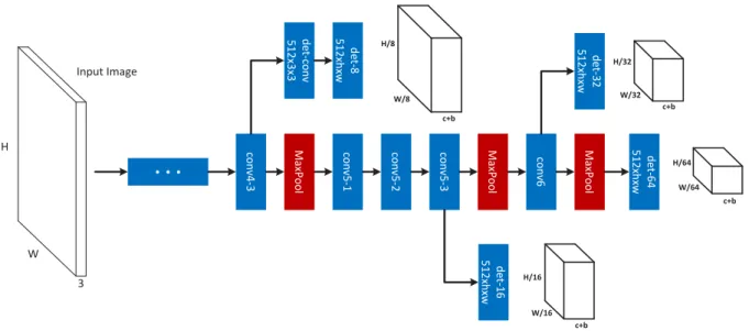
W H 3 Input Image conv 4 -3 Max Poo l conv 5 -1 conv 5 -2 conv 5 -3 det -conv 512 x3 x3 Max Poo l conv 6 det -8 512 xhxw · · · d e t-16 5 1 2 xh xw Max Poo l det -32 512 xh xw d et -6 4 5 1 2 xh xw H/8 c+b W/8 c+b H/64 W/64 H/32 c+b W/32 H/16 c+b W/16

Figure 2.3: Proposal sub-network of the MS-CNN. The bold cubes are the output tensors of

the network.h×wis the filter size,cthe number of classes, andbthe number of bounding box coordinates.

compromises object detection performance.

Inspired by previous evidence on the benefits of the strategy of Figure 2.2 (c) over that of Figure 2.2 (b), we propose a new multi-scale strategy, shown in Figure 2.2 (g). This can be seen as the deep CNN extension of Figure 2.2 (c), but only uses a single scale of input. It differs from both Figure 2.2 (e) and (f) in that it exploits feature maps of several resolutions to detect objects at different scales. This is accomplished by the application of a set of templates at intermediate network layers. This results in a set of variable receptive field sizes, which can cover a large range of object sizes.

2.3.2

Architecture

The detailed architecture of the MS-CNN proposal network is shown in Figure 2.3. The network detects objects through several detection branches. The results by all detection branches are simply declared as the final proposal detections. The network has a standard CNN trunk, depicted in the center of the figure, and a set of output branches, which emanate from different

(38)

layers of the trunk. These branches consist of a single detection layer. Note that a buffer convolutional layer is introduced on the branch that emanates after layer “conv4-3”. Since this branch is close to the lower layers of the trunk network, it affects their gradients more than the other detection branches. This can lead to some instability during learning. The buffer convolution prevents the gradients of the detection branch from being back-propagated directly to the trunk layers.

During training, the parameters W of the multi-scale proposal network are learned

from a set of training samples S = {(X_i,Y_i)}N

i=1, where Xi is a training image patch, and

Y_i= (y_i,b_i) the combination of its class label y_i ∈ {0,1,2,· · ·,K} and bounding box

coordi-natesbi= (bx_i,b_iy,bw_i ,bh_i). This is achieved with a multi-task loss

L

(W) =

M

∑

m=1i∈

∑

Sm

αmlm(Xi,Yi|W), (2.1)

whereMis the number of detection branches,αmthe weight of losslm, andS={S1,S2,· · ·,SM},

whereSmcontains the examples of scalem. Note that only a subsetSmof the training samples,

selected by scale, contributes to the loss of detection layerm. Inspired by the success of joint

learning of classification and bounding box regression [50, 140], the loss of each detection layer combines these two objectives

l(X,Y|W) =L_cls(p(X),y) +λ[y≥1]Lloc(b,bˆ), (2.2)

where p(X) = (p0(X),· · ·,pK(X)) is the probability distribution over classes, λ a trade-off

coefficient,L_cls(p(X),y) =−logp_y(X)the cross-entropy loss, ˆb= (bˆ_x,bˆ_y,bˆ_w,bˆ_h)the regressed bounding box, and

L_loc(b,bˆ) =1

4

∑

j∈{x,y,w,h}

smooth_L₁(b_j,bˆ_j), (2.3)

(39)

positive samples and the optimal parameters W∗=arg minW

L

(W) are learned by stochastic

gradient descent.

2.3.3

Sampling

This section describes the assembly of training samplesSm={S₊m,Sm₋}for each detection

layer m. In what follows, the superscriptm is dropped for notional simplicity. An anchor is

centered at the sliding window on layermassociated with width and height corresponding to filter

size. More details can be found in Table 2.1. A sampleX of anchor bounding boxbis labeled as

positive ifo∗≥0.5, where

o∗=max i∈Sgt

IoU(b,b_i). (2.4)

S_gt is the ground truth andIoU the intersection over union between two bounding boxes. In

this case,Y = (yi∗,b_i∗), wherei∗=arg max_i_∈_S_gtIoU(b,b_i)and(X,Y)are added to the positive

set S+. All the positive samples inS+={(Xi,Yi)|yi≥1}contribute to the loss. Samples such

that o∗<0.2 are assigned to a preliminary negative training pool, and the remaining samples

discarded. For a natural image, the distribution of objects and non-objects is heavily asymmetric. Sampling is used to compensate for this imbalance. To collect a final set of negative samples

S₋ ={(X_i,Y_i)|y_i=0}, such that|S₋|=γ|S+|, we considered three sampling strategies: random,

bootstrapping, and mixture.

Random sampling consists of randomly selecting negative samples according to a uniform distribution. Since the distribution of hard and easy negatives is heavily asymmetric too, most randomly collected samples are easy negatives. It is well known that hard negatives mining helps boost performance, since hard negatives have the largest influence on the detection accuracy. Bootstrapping accounts for this, by ranking the negative samples according to their objectness

scores, and then collecting top|S₋|negatives. Mixture sampling combines the two, randomly

(40)

sampling has very similar performance to bootstrapping.

To guarantee that each detection layer only detects objects in a certain range of scales,

the training set for the layer consists of the subset ofSthat covers the corresponding scale range.

For example, the samples of smallest scale are used to train the detector of “det-8” in Figure 2.3. It is possible that no positive training samples are available for a detection layer, resulting

in|S₋|/|S₊| γ. This can make learning unstable. To address this problem, the cross-entropy

terms of positives and negatives are weighted as follows

L_cls= 1 1+γ 1 |S+|_i_∈

∑

_S₊ −logpyi(Xi) + γ 1+γ 1 |S₋|_i_∈

∑

_S − −logp0(Xi). (2.5)

2.3.4

Implementation Details

Data Augmentation: In [50, 59], it is argued that multi-scale training is not needed, since deep neural networks are adept at learning scale invariance. This, however, is not true for datasets such as Caltech [32] and KITTI [43], where object scales can span multiple octaves.

In KITTI, many objects are quite small. Without rescaling, the cardinalities of the sets S+=

{S1₊,S₊2,· · ·,S₊M}are wildly varying. In general, the set of training examples of largest object size is very small. To ease this imbalance, the original images are randomly resized to multiple scales.

Fine-tuning: Training the Fast-RCNN [50] and RPN [140] networks requires large

amounts of memory and a small mini-batch, due to the large size of the input (i.e. 1000×600).

This leads to a very heavy training procedure. In fact, many background regions that are useless for training take substantially amounts of memory. Thus, we randomly crop a small patch

(e.g. 448×448) around objects from the whole image. This drastically reduces the memory

requirements, enabling four images to fit into the typical GPU memory of 12G.

Learning is initialized with the popular VGG-Net [150]. Since bootstrapping and the multi-task loss can make training unstable in the early iterations, a two-stage procedure is adopted.

(41)

H/4 W/4 7 512 conv4-3-2x Fu lly Co nn ected 7 512 b o u nd in g b ox class probab ilit y 5 5 512 ROI-Polling 512 H/8 W/8 512 conv4-3 Deconvolution · · · trunk CNN layers

Figure 2.4: Object detection sub-network of the MS-CNN. “trunk CNN layers” are shared with

proposal sub-network.W andHare the width and height of the input image. The green (blue) cubes represent object (context) region pooling.

iterations are run with a learning rate of 0.00005. The resulting model is used to initialize the

second stage, where random sampling is switched to bootstrapping andλ=1. We setαi=0.9 for

“det-8” andαi=1 for the other layers. Another 25,000 iterations are run with an initial learning

rate of 0.00005, which decays 10 times after every 10,000 iterations. This two-stage learning procedure enables stable multi-task training.

2.4

Object Detection Network

Although the proposal network could work as a detector itself, it is not strong, since its sliding windows do not cover objects well. To increase detection accuracy, a detection network is added. Following [50], a ROI pooling layer is first used to extract features of a fixed dimension

(e.g. 7×7×512). The features are then fed to a fully connected layer and output layers, as shown

in Figure 2.4. A deconvolution layer, described in Section 2.4.1, is added to double the resolution of the feature maps. The multi-task loss of (2.1) is extended to

L

(W,Wd) = M

∑

m=1i∈

∑

Sm αmlm(Xi,Yi|W) +

∑

i∈SM+1 αM+1lM+1(Xi,Yi|W,Wd), (2.6)

(42)

wherelM+1 and SM+1 are the loss and training samples for the detection sub-network. SM+1

is collected as in [50]. As in (2.2), lM+1combines a cross-entropy loss for classification and

a smoothed L1 loss for bounding box regression. The detection sub-network shares some of

the proposal sub-network parameters Wand adds some parametersW_d. The parameters are

optimized jointly, i.e. (W∗,W∗_d) =arg min

L

(W,Wd). In the proposed implementation, ROI

pooling is applied to the top of the “conv4-3” layer, instead of the “conv5-3” layer of [50], since “conv4-3” feature maps performed better in our experiments. One possible explanation is that “conv4-3” corresponds to higher resolution and is better suited for location-aware bounding box

regression.

2.4.1

CNN Feature Map Approximation

Input size has a critical role in CNN-based object detection accuracy. Simply forwarding object patches, at the original scale, through the CNN impairs performance (especially for small

ones), since the pre-trained CNN models have a natural scale (e.g. 224×224). While the R-CNN

naturally solves this problem through warping [51], it is not explicitly addressed by the Fast-RCNN [50] or Faster-Fast-RCNN [140]. To bridge the scale gap, these methods simply upsample

input images (by∼2 times). For datasets, such as KITTI [43], containing large amounts of small

objects, this has limited effectiveness. Input upsampling also has three side effects: large memory requirements, slow training and slow testing. It should be noted that input upsampling does not enrich the image details. Instead, it is needed because the higher convolutional layers respond

very weakly to small objects. For example, a 32×32 object is mapped into a 4×4 patch of the

“conv4-3” layer and a 2×2 patch of the “conv5-3” layer. This provides limited information for

7×7 ROI pooling.

To address this problem, we consider an efficient way to increase the resolution of feature maps. This consists of upsampling feature maps (instead of the input) using a deconvolution layer, as shown in Figure 2.4. This strategy is similar to that of [29], shown in Figure 2.2 (d), where

(43)

input rescaling is replaced by feature rescaling. In [29], a feature approximator is learned by least squares. In the CNN world, a better solution is to use a deconvolution layer, similar to that of [107]. Unlike input upsampling, feature upsampling does not incur in extra costs for memory and computation. Our experiments show that the addition of a deconvolution layer significantly boosts detection performance, especially for small objects. To the best of our knowledge, this is the first application of deconvolution to jointly improve the speed and accuracy of an object detector.

2.4.2

Context Embedding

Context has been shown useful for object detection [46, 16, 2] and segmentation [198]. Context information has been modeled by a recurrent neural network in [2] and acquired from multiple regions around the object location in [46, 16, 198]. In this work, we focus on context from multiple regions. As shown in Figure 2.4, features from an object (green cube) and a context (blue cube) region are stacked together immediately after ROI pooling. The context region is 1.5 times larger than the object region. An extra convolutional layer without padding is used to reduce the number of model parameters. It helps compress redundant context and object information, without loss of accuracy, and guarantees that the number of model parameters is approximately the same.

2.4.3

Implementation Details

Learning is initialized with the model generated by the first learning stage of the proposal network, described in Section 2.3.4. The learning rate is set to 0.0005, and reduced by a factor of 10 times after every 10,000 iterations. Learning stops after 25,000 iterations. The joint optimization of (2.6) is solved by back-propagation throughout the unified network. Bootstrapping

(44)

Table 2.1: Parameter configurations of the different models.

det-8 det-16 det-32 det-64 ROI FC

car filter 5x5 7x7 5x5 7x7 5x5 7x7 5x5 7x7 4096 anchor 40x40 56x56 80x80 112x112 160x160 224x224 320x320 ped/cyc filter 5x3 7x5 5x3 7x5 5x3 7x5 5x3 7x5 2048 anchor 40x28 56x36 80x56 112x72 160x112 224x144 320x224 caltech filter 5x3 7x5 5x3 7x5 5x3 7x5 5x3 8x4 2048 anchor 40x20 56x28 80x40 112x56 160x80 224x112 320x160

during learning, for faster training.

2.5

Experimental Evaluation

The performance of the MS-CNN detector was evaluated on the KITTI [43] and Caltech Pedestrian [32] benchmarks. These were chosen because, unlike VOC [36] and ImageNet [143],

they contain many small objects. Typical image sizes are 1250×375 on KITTI and 640×480

on Caltech. KITTI contains three object classes: car, pedestrian and cyclist, and three levels of evaluation: easy, moderate and hard. The “moderate” level is the most commonly used. In total, 7,481 images are available for training/validation, and 7,518 for testing. Since no ground truth is available for the test set, we followed [16], splitting the trainval set into training and validation sets. In all ablation experiments, the training set was used for learning and the validation set for evaluation. Following [16], a model was trained for car detection and another for pedestrian/cyclist detection. One pedestrian model was learned on Caltech. The model configurations for original input size are shown in Table 2.1. The detector was implemented in C++ within the Caffe toolbox [76], and source code is available at https://github.com/zhaoweicai/mscnn. All times are reported for implementation on a single CPU core (2.40GHz) of an Intel Xeon E5-2630 server with 64GB of RAM. An NVIDIA Titan GPU was used for CNN computations.

(45)

Table 2.2: Detection recall of the various detection layers on KITTI validation set (car), as a function of object hight in pixels.

det-8 det-16 det-32 det-64 combined 25≤height<50 0.9180 0.3071 0.0003 0 0.9360 50≤height<100 0.5934 0.9660 0.4252 0 0.9814 100≤height<200 0.0007 0.5997 0.9929 0.4582 0.9964 height≥200 0 0 0.9583 0.9792 0.9583 all scales 0.6486 0.5654 0.3149 0.0863 0.9611 100 101 102 103 0 0.2 0.4 0.6 0.8 1 # candidates

recall at IoU threshold 0.7

RPN−h384 h384 h384−mt h576−mt h768−mt Car 100 101 102 103 0 0.2 0.4 0.6 0.8 1 # candidates

RPN−h384 h384 h384−mt h576−mt h768−mt Pedestrian 100 101 102 103 0 0.2 0.4 0.6 0.8 1 # candidates

RPN−h384 h384 h384−mt h576−mt h768−mt Cyclist

Figure 2.5: Proposal recall on the KITTI validation set (moderate). “hXXX” refers to input

images of height “XXX”. “mt” indicates multi-task learning of proposal and detection sub-networks.

2.5.1

Proposal Evaluation

We start with an evaluation of the proposal network. Following [63], oracle recall is used as performance metric. For consistency with the KITTI setup, a ground truth is recalled if its best

matched proposal hasIoU higher than 70% for cars, and 50% for pedestrians and cyclists.

The roles of individual detection layers: Table 2.2 shows the detection accuracy of the various detection layers as a function of object height in pixels. As expected, each layer has highest accuracy for the objects that match its scale. While the individual recall across scales is low, the combination of all detectors achieves high recall for all object scales.

The effect of input size: Figure 2.5 shows that the proposal network is fairly robust to the size of input images for cars and pedestrians. For cyclist, performance increases between heights 384 and 576, but there are no gains beyond this. These results show that the network can

(46)

100 101 102 103 104 0 0.2 0.4 0.6 0.8 1 # candidates

BING MCG EB SS 3DOP RPN MS−CNN 100 101 102 103 104 0 0.2 0.4 0.6 0.8 1 # candidates

BING MCG EB SS 3DOP RPN MS−CNN 0.5 0.6 0.7 0.8 0.9 1 0 0.2 0.4 0.6 0.8 1

IoU overlap threshold

recall BING 1.7 MCG 21.8 EB 10.8 SS