Utah State University Utah State University
DigitalCommons@USU
DigitalCommons@USU
All Graduate Plan B and other Reports Graduate Studies 5-2013
Probability Estimation in Random Forests
Probability Estimation in Random Forests
Chunyang LiUtah State University
Follow this and additional works at: https://digitalcommons.usu.edu/gradreports
Part of the Statistics and Probability Commons
Recommended Citation Recommended Citation
Li, Chunyang, "Probability Estimation in Random Forests" (2013). All Graduate Plan B and other Reports. 312.
https://digitalcommons.usu.edu/gradreports/312 This Thesis is brought to you for free and open access by the Graduate Studies at DigitalCommons@USU. It has been accepted for inclusion in All Graduate Plan B and other Reports by an authorized administrator of DigitalCommons@USU. For more information, please contact [email protected].
Probability Estimation in Random Forests
by Chunyang Li
A thesis submitted in partial fulfillment of the requirements for the degree
of
MASTER OF SCIENCE in
Statistics
Approved:
Adele Cutler Yan Sun
Major Professor Committee Member
John R. Stevens Committee Member
UTAH STATE UNIVERSITY Logan, Utah
ii
Copyright c Chunyang Li 2013 All Rights Reserved
iii ABSTRACT
Probability Estimation in Random Forests
by
Chunyang Li, Master of Science Utah State University, 2013
Major Professor: Dr. Adele Cutler Department: Mathematics and Statistics
Random Forests is a useful ensemble approach that provides accurate predictions for classification, regression and many different machine learning problems. Classification has been a very useful and popular application for Random Forests. However, it is preferable to have the probability of a membership rather than the simple knowledge that one belongs to whichever group. Votes and the regression method are current probability estimation methods that have been developed in Random Forests. In this thesis, we introduce two new methods, proximity weighting and the out-of-bag method, trying to improve the cur-rent methods. Several diffecur-rent simulations are designed to evaluate the new methods and compare them with the old ones. Finally, we use real data sets from UCI machine learning repository to further evaluate and compare those methods.
iv
v ACKNOWLEDGMENTS
I would like to thank my advisor, Dr. Adele Cutler, for your patience on me and the time you spent helping me with this research. Thanks for setting me an awesome example of academic excellence, enthusiasm and work ethic. Thanks for giving me advice on everything for my current study and future career.
I would also like to thank my committee members, Dr. Sun and Dr. Stevens, for your help on a lot of my course work that make me better prepared for this research. Thanks for all your advice and your time being my committee members.
Finally, I would like to thank all my officemates and friends in the department, who help me and give me a lot of support. Thank my roommates for giving me great friendship and encouraging me.
vi CONTENTS Page ABSTRACT . . . iii DEDICATION . . . iv ACKNOWLEDGMENTS . . . v
LIST OF TABLES . . . viii
LIST OF FIGURES . . . ix 1 Introduction . . . 1 1.1 Classification . . . 1 1.2 Probability Estimation . . . 1 1.3 Trees . . . 2 1.4 Random Forests . . . 3
2 Probability Estimation Methods . . . 6
2.1 Voting . . . 6 2.2 Probability Machines . . . 6 2.3 Proximity Weighting . . . 6 2.4 Out-of-bag Method . . . 7 2.5 Software . . . 7 3 Simulation . . . 8
3.1 XOR model ( XOR1and XOR2 ) . . . 8
3.2 2-dimensional Circle Model(2D Circle) . . . 9
3.3 10-dimensional Model (Friedman) . . . 9
3.4 Bivariate Normal Model (Binorm) . . . 10
3.5 Normal Cluster Mixtures(Clusters) . . . 11
3.6 Method to Measure the Performance of Class Probability Estimators . . . 12
3.6.1 Mean Squared Loss Function . . . 12
3.6.2 Misclassification Error Rate . . . 13
3.7 Simulation results . . . 14
3.7.1 Results for Mean Squared Loss . . . 14
3.7.2 Results for Misclassification Error Rate . . . 15
3.7.3 Normal Cluster Mixtures with Different Ntrees . . . 16
4 Data Examples. . . 17
4.1 Brier Score . . . 17
4.2 10-fold Cross Validation . . . 17
4.3 Missing Values . . . 17
vii
4.3.2 RfImpute . . . 18
4.4 Results for Real Data . . . 18
5 Conclusions . . . 21
6 Discussion and Future Work . . . 23
viii LIST OF TABLES
Table Page
3.1 Mean Squared Loss N=100 . . . 14
3.2 Mean Squared Loss N=500 . . . 14
3.3 Mean Squared Loss N=1000 . . . 14
3.4 Misclassification Error Rate N=100 . . . 15
3.5 Misclassification Error Rate N=500 . . . 15
3.6 Misclassification Error Rate N=1000 . . . 15
3.7 Mean Squared Loss for Normal Cluster Mixtures with Different Ntrees . . . 16
3.8 Misclassification Error Rate for Normal Cluster Mixtures with Different Ntrees 16 4.1 Brier Score(Missing values are replaced using rfImpute) . . . 19
ix LIST OF FIGURES
Figure Page
3.1 XOR Model . . . 9 3.2 Training data (left) and true probabilities of being in class 1 (right) for the
2-Dimensional Circle Model . . . 10 3.3 Bivariate Normal Model . . . 12 3.4 Normal Cluster Mixtures . . . 13
CHAPTER 1 INTRODUCTION 1.1 Classification
Classification is the problem of predicting which class a new observation belongs to, given a training set of data fromK known classes. One way to think about classification is that it’s like regression but we have a categorical response variable instead of a continuous response.
Assume we have a sample (x1, y1), . . . ,(xN, yN) of independent and identically dis-tributed observations, where xi = (xi1, . . . , xiM)T ∈ X ⊆ RM and yi ∈ {1, . . . , K} for
i = 1, . . . , N. The values of yi refer to the classes and the problem is to classify a new
observationxnew into one of theK classes, i.e. to estimate ˆynew. No formal distributional
assumptions are made, although there are implicit assumptions that “nearby” values of x
provide information about y.
1.2 Probability Estimation
Most machine learning approaches only provide a classification result. However, it is not enough and probabilities are essential in some cases like predicting diseases. It is important to estimate the probability of belonging to each of the groups rather than making a simple statement that a patient is in one group or another. Therefore, our research problem is using Random Forests to get the most accurate probability estimates.
More formally, letfk(x) denote the density function for observations in class k. Then
f(x) =
k
X
k=1
πkfk(x)
where 0 ≤ πk ≤ 1 and PKk=1πk = 1. We can view the data (x1, y1), . . . ,(xN, yN) as
realizations of random variables (x, y), where
P(y=k) =πk
and
2 so
f(x) =X
k
πkfk(x)
As well as predicting y when X =xnew, we would like to estimate
pk=P(y=k|X =xnew)
= πkfk(xnew)
f(x)
1.3 Trees
A classification tree is usually grown by firstly considering a “root” node containing all the observations. Observations in the node are sent to the descendant nodes, using a “split” on a single predictor variable. The initial (“root”) node contains the data of interest and nodes that can’t be split are called “terminal” nodes. At any stage of the tree-growing process, a node contains observations in some or all of the classes {1, . . . , K} and the y -values in the node can be summarized by a vector n = (n1, . . . , nK)T where nk is the
number of observations of class kin the node.
Considering every possible split on every predictor variable, a particular split of a node is chosen. The predictor and split combination giving the “best” value according to some criterion, such as Gini index, entropy, etc., is used to partition the node. In this report, we use the Gini Index.
For continuous predictors, each split is of the formxj < cfor somecandj∈ {1, . . . , M}, where xj denotes the value of variable j. Observations that have xj < c go to the left descendant node, and the others go to the right. The values of j and c for each node are found by minimizing a measure of the “badness” of the split based on the Gini index. For a node whosey-values are summarized byn= (n1, . . . , nK)T of sizeS=PKk=1nk, the Gini
index is G(n) = X k6=k0 nk N nk0 N .
3 and nR = nR(c, j) with size SL and SR where SL+SR = S. The values of c and j are chosen to minimize
SLG(nL) +SRG(nR).
Denoting the sorted sample values of variable j in the node by x(1)j, . . . , x(S)j, the
minimization is performed over
c∈
(x(i)j+x(i+1)j)/2, i= 1, . . . , S−1 .
For stand-alone trees, the minimization is performed over j ∈ {1, . . . , M}. In random forests, the minimization is performed over j in a random subset of {1, . . . , M}, chosen independently at each node. Typically, the size of the subset is close to √M.
The minimization over both j and c is performed using an exhaustive search over all combinations ofcandjas described above. For a given variablej, the Gini index is updated as we move through the possible values ofc from smallest to largest.
The trees are usually grown until a stopping criterion is met, or the nodes contain a small enough number of cases.
To predict the class of xnew, we start from the root node and move down the tree. At
a node, if thejth component ofxnew satisfies the appropriate condition, it goes to the left,
otherwise it goes to the right. In this way,xnew ends up in a terminal node. The predicted class at the terminal node is the most popular class among the training data at the node with ties broken at random.
1.4 Random Forests
The Random Forest method was introduced by Leo Breiman in 2001 [1] and is a very useful tool for machine learning. It is a combination of tree predictors such that each tree depends on the information of a bootstrap sample from the original data (training set). It can be used for classification and regression. Here, we are only considering Classification Random Forests.
4 Trees like those described in sections 1.3 are used in Random Forests as described in the following. The parameters ntree and m (the number of must be chosen. The value of ntree, the number of trees in the forest, can be chosen as large as desired. There is no penalty, in terms of fit, for choosing ntree too large, but the fit may be poor if it is too small. The default value of ntree in the R implementation is 500. The value ofm, which controls the number of randomly chosen predictors at each node (as described in Section 1.3), is usually taken to be an integer close to √M.
To construct the forest, suppose we have a training set (x1, y1), . . . ,(xN, yN) and let A= {1, . . . , N}. Then fort in 1, . . . ,ntree:
1. Take a bootstrap sample from the data (sample N times, at random, with replace-ment).
2. Denote the set of observations appearing in the bootstrap sample byBt⊂A.
3. Denote the set of observationsnotappearing in the bootstrap sample byBct =A\Bt.
4. Fit a classification tree (Section 1.3) to the bootstrap sample, splitting until all the observations in each terminal node come from the same class (“pure”).
5. Find the predicted class at each terminal node (the class of members of Bt in the node).
6. For each member of Btc, pass it down the tree. 7. Letqt(i) denote the terminal nodes for alli∈A.
The predicted class for observations in the training set is the most frequent class in the trees for which the observation is a member of Btc. This process is often described as “voting” the trees. For new observations, all the trees in the forest are used in the voting. The observations inBtcare said to be “out-of-bag” for treet. The “out-of-bag” error rate is the
5 error rate of the Random Forest predictions for the training set. These predictions are also used to give the “out-of-bag” confusion matrix.
Let the proximity between the ith and jth observations be the proportion of the time observationsiandjare in the same terminal node, where the proportion is taken over trees for which iand j are inBtc(i.e. both out-of-bag):
prox(i, j) =
Pntree
t=1 I(i∈Bct)I(j∈Btc)I(qt(i) =qt(j))
Pntree
t=1 I(i∈Btc)I(j ∈Btc)
whereI denotes the indicator function. To find the proximity between an observation from the training set, and one from the test set, we use
prox(i, j) = 1 ntree ntree X t=1 I(qt(i) =qt(j)).
6 CHAPTER 2
PROBABILITY ESTIMATION METHODS
Let pi,k =P(Y = k|X = xi}. We compare four methods of estimating pi,k. The first
method, based on voting the trees, is the “standard” or “default” method. The second method is a regression method introduced by Malley et al. [10]. The third and fourth methods, labeled “Proximity Weighting” and “Out-of-bag” are new methods developed for this research project.
2.1 Voting
For test data, ˆpvotei,k is the proportion of trees that predict classk when observationxi
is passed down the tree. For training data, the proportion is only taken over trees for which
xi is out-of-bag.
2.2 Probability Machines
This method only works for two-class problems (K = 2). The two classes are denoted 0 and 1 and Random Forests is run in regression mode. Random Forests for regression are analogous to Random Forests for classification, except that the splits are chosen to minimize the mean squared error instead of Gini, the predictions for a tree are the average of the y-values of Bt in the nodes, and the predicted values for the forest are obtained by averaging over the trees for which the observation is in Bct. Once the Random Forests regression predictions{y1, . . . ,ˆ yNˆ } are obtained, we set ˆpregi,1 = ˆyi and ˆpregi,0 = 1−yiˆ.
2.3 Proximity Weighting
The motivation for this method comes from the fact that Random Forests can be thought of as a “nearest neighbor” classifier [4] and proximities are believed to correspond to the neighborhoods of the nearest neighbor classifier. The proximity weighting method uses the proximities defined above to find a weighted average:
7 ˆ pproxi,k = P j∈A,j6=iprox(i, j)I(yj =k) P j∈A,j6=iprox(i, j) .
The weighted average means that observations that are “close” have more impact on the probability estimate than observations that are not “close” (where “close” is defined using the Random Forest proximities). For more information about proximities, see A. Cutler et al.[2]
2.4 Out-of-bag Method
The motivation for this method comes from the fact that when fitting a classifier using a single tree, the terminal nodes are not pure and the relative frequency of class k in a terminal node can be used to estimate the probability of class k for observations in that terminal node. In Random Forests, the terminal nodes are pure so the information from members of Bt is not useful. However, the out-of-bag observations (those in Btc) do give
information about the underlying class probabilities.
For treet, if a node contains members of Btc, we use the relative frequency of class k
observations in Btcin node qt to estimate the probabilities for the node:
ˆ pqt,k= P j∈Bc t I(qt(j) =qt)I(ˆyj =k) P j∈Bc t I(qt(j) =qt) .
and denote the set of nodes that do not contain members of Btc by Q0t. The out-of-bag estimates of the probabilities are found by averaging over the nodes that contain out-of-bag observations: ˆ poobi,k = Pntree t=1 I(qt(i)∈/Q0t)ˆpqt(i),k Pntree t=1 I(qt(i)∈/Q0t) . 2.5 Software
8 CHAPTER 3
SIMULATION
The simulation designs are used to represent scenarios where a binary response variable
Y is predicted from a set of predictor variables.
We used five simulation models in order to compare the probability estimation methods. The first one is the XOR model. The second and the third one are from Mease et al. [11], where they considered a simple two-dimensional circle model and 10 dimensional model. The fourth one is a bivariate normal mixture model and the last one is a mixture of normal clusters taken from the Elements of Statistical Learning [5]. We also make the plots for each model to visualize them.
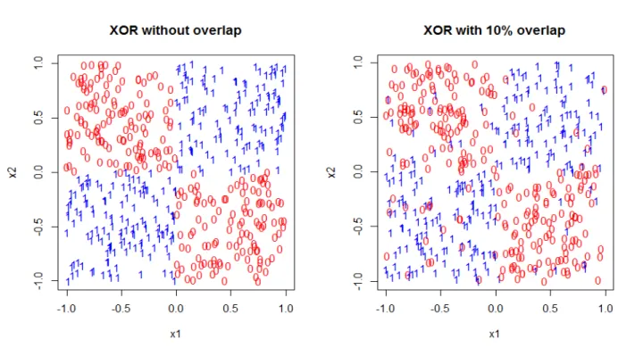
3.1 XOR model ( XOR1and XOR2 )
Let X = (X1, X2) be a two-dimensional random vector uniformly distributed on the
square [−1,1]2 and lety be a categorical variable with values 0 or 1 defined as
y=
0 x1x2 ≤0;
1 x1x2 >0.
Y = 0 corresponds to class 0 andY = 1 corresponds to class 1.Therefore, the conditional probability ofY = 1 given X is
P(y= 1|X =x) =
0 x1x2 ≤0; 1 x1x2 >0.
A second case of the XOR model is overlapping 10% based on the the model described above. We sample 10% observations from class 0 without replacement and switch it with the same number of observations from class 1. The conditional probabilityY = 1 given X
is: P(y= 1|X=x) = 0.1 x1x2 ≤0; 0.9 x1x2 >0. .
9
Figure 3.1. XOR Model 3.2 2-dimensional Circle Model(2D Circle)
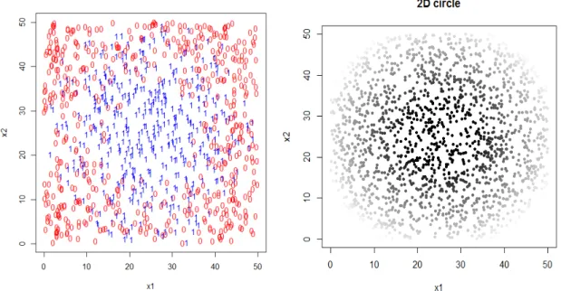
LetXbe a two-dimensional random vector uniformly distributed on the square [0,50]2and Y be a categorical variable with values 0 or 1 depending on X. We construct level curves of p(x) to be concentric circles with center (25, 25). The conditional probability of Y = 1 given X=x is defined as:
P(Y = 1|X =x) = 1 r(x)<8; 28−r(x) 20 8≤r(x)≤28; 0 r >28.
wherer(x) is the distance fromxto the point (25, 25) inR2. This is called the 2-Dimensional Circle model. The right panel of figure3.2 shows these probabilities for a hold-out sample with that is a grid 2000 evenly spaced points on [0,50]2. The greyness of the plot shows the probabilities: the lighter the color is, the smaller the probabilities are.
3.3 10-dimensional Model (Friedman)
Let X be a 10-dimensional random vectorX = (X1, X2..., X10) distributed according to N10(0, I) and let Y be a categorical variable with values 0 or 1 depending on X. The
10
Figure 3.2. Training data (left) and true probabilities of being in class 1 (right) for the 2-Dimensional Circle Model
conditional probability that Y = 1 given X = x (which we denote p(x)) is defined as follows: log p(x) 1−p(x) =r[1−x1+x2−x3+x4−x5+x6] 6 X j=1 xj
We choose r=10, which mimics the simulation of Friedman’s model exactly. [6]
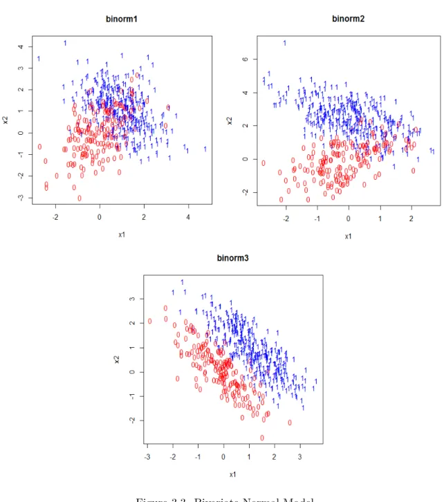
3.4 Bivariate Normal Model(Binorm)
Let X be a random matrix consisting of two classes that belong to two different bi-variate normal distributions with mean µ0 and µ1 and covariance Σ0 and Σ1. Let Y be
a dichotomous dependent variable with Y = 0 corresponding to class 0 and Y = 1 cor-responding to class 1. The conditional probability that Y = 1 given X =x is defined as:
f(Y = 1|X =x) = π1f1(x)
π0f0(x) +π1f1(x)
where π0 and π1 are the probabilities thatY = 0 and Y = 1 respectively, f0(x) and f1(x)
are the probability density functions of class 0 and class 1.
11
and binorm3. Binorm1 has class 0 with meanµ0 = (0,0)T, covariance Σ0 =
1 0.55 0.55 1
and class 1 with mean µ1 = (0,2.5)T, covariance Σ1 =
1 −0.55
−0.55 1
. Binorm2 has class 0 with mean µ0 = (0,0)T, covariance Σ0 =
1 0.47 0.47 1
and class 1 with mean
µ1 = (1,1)T, covariance Σ1 =
1 −0.47
−0.47 1
. Binorm3 has class 0 with mean µ0 =
(0,0)T, covariance Σ0 =
1 −0.8
−0.8 1
and class 1 with mean µ1 = (1,1)T, covariance Σ1=
1 −0.8
−0.8 1
. Class 0 is generated with probabilityπ0= 2/3 for the three cases.
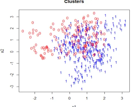
3.5 Normal Cluster Mixtures (Clusters)
Let a 2-dimensional vectorX ={X1, X2}. Firstly 10 meansµj ={muj1, . . . , µj10}are
generated from a bivariate normal distributionN2((1,0)T,I) and 10 more meansµi{mui1, . . . , µi10}
are drawn from another bivariate normal distribution N2((0,1)T,I). We are generating a
sample with N observations in total and the sample sizes for class 0 and class 1 aren0 and n1. Then for each class, we generaten0 andn1 observations as follows: for each observation, a mean µis picked at random with probability 1/10 from {muj1, . . . , µj10} for class 0 and from {mui1, . . . , µi10}for class 1. Then the observation is drawn from a new bivariate nor-mal distribution with the selected mean and covariance Σ =I/5. Y is the binary response variable, whereY = 0 corresponds to class 0 andY = 1 corresponds to class 1.
The conditional probability that Y = 1 given X = x is calculated using the same formula given above in the multivariate normal model. However, f0(x) and f1(x) are not
directly given and they are the average of the pdf’s of 10 different bivariate normal distri-butions.
In our simulation, class 0 is generated with probability π0 = 2/3. The plot below is a sample with N=500.
12
Figure 3.3. Bivariate Normal Model 3.6 Method to Measure the Performance of Class
Probability Estimators
3.6.1 Mean Squared Loss Function
We choose mean squared loss function to quantify the accuracy of the probability estimates for the simulations. It is defined:
1 N N X i=1 (p(xi)−pˆ(xi))2
13
Figure 3.4. Normal Cluster Mixtures 3.6.2 Misclassification Error Rate
Another way we use to measure the accuracy of the probability estimates for the simulations is misclassification error rate. We give the classification results according the the probability estimations, i.e. an observation belongs to the class with bigger probability. The trees are built based on the simulation training data with sample size N. There are 500 trees in total for each case, i.e. ntree=500. Changing ntree didn’t change the squared loss for each method from the early experiments we did (Section 3.7.3), therefore, we are only showing the results when ntree=500. We use the test data from 100 independent sample with sample size 1000 to evaluate the probability estimates. The final mean squared loss of the sample is the average of the losses for the 100 times’ simulations. So does the misclassification error rate.
14 3.7 Simulation results
3.7.1 Results for Mean Squared Loss
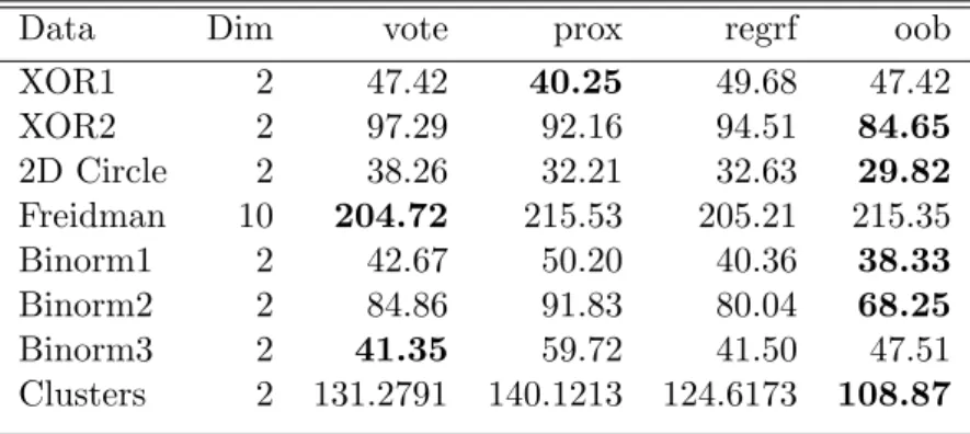
Table 3.1. Mean Squared Loss N=100
Data Dim vote prox regrf oob
XOR1 2 47.42 40.25 49.68 47.42 XOR2 2 97.29 92.16 94.51 84.65 2D Circle 2 38.26 32.21 32.63 29.82 Freidman 10 204.72 215.53 205.21 215.35 Binorm1 2 42.67 50.20 40.36 38.33 Binorm2 2 84.86 91.83 80.04 68.25 Binorm3 2 41.35 59.72 41.50 47.51 Clusters 2 131.2791 140.1213 124.6173 108.87
Table 3.2. Mean Squared Loss N=500
Data Dim vote prox regrf oob
XOR1 2 7.85 4.89 7.99 7.72 XOR2 2 80.09 74.65 77.09 66.39 2D Circle 2 28.93 21.74 24.18 13.36 Freidman 10 164.46 168.69 165.19 184.75 Binorm1 2 37.94 43.02 35.60 30.23 Binorm2 2 77.3477 86.0702 72.7500 60.79 Binorm3 2 23.78 32.54 22.66 22.88 Clusters 2 135.38 144.36 130.67 115.27
Table 3.3. Mean Squared Loss N=1000
Data Dim vote prox regrf oob
XOR1 2 3.35 2.00 3.41 3.27 XOR2 2 79.33 64.89 76.37 60.50 2D Circle 2 26.96 20.25 22.36 10.34 Freidman 10 147.14 146.15 148.17 167.81 Binorm1 2 35.95 40.27 33.86 28.40 Binorm2 2 75.45 86.41 71.20 59.81 Binorm3 2 21.40 27.78 20.18 19.24 Clusters 2 138.87 150.15 134.50 120.74
The data in the tables are all in 10−3 scale, i.e. the real mean squared lost should be the value in the table times 0.001. All the simulation data only have two classes, i.e.
15 response variable with 2 categories. The bolded value is the smallest mean squared loss in a row.
3.7.2 Results for Misclassification Error Rate
Table 3.4. Misclassification Error Rate N=100
Data Dim vote prox regrf oob
XOR1 2 0.0419 0.0412 0.0423 0.0344 XOR2 2 0.1898 0.1802 0.1856 0.1651 2D Circle 2 0.2669 0.2585 0.2595 0.2542 Freidman 10 0.3742 0.3984 0.3760 0.4009 Binorm1 2 0.1098 0.1028 0.1067 0.1026 Binorm2 2 0.2041 0.1853 0.1972 0.1855 Binorm3 2 0.0915 0.1103 0.0917 0.0946 Clusters 2 0.3053 0.2841 0.2992 0.2826
Table 3.5. Misclassification Error Rate N=500
Data Dim vote prox regrf oob
XOR1 2 0.00561 0.00524 0.00563 0.00523 XOR2 2 0.12767 0.11224 0.12136 0.11089 2D Circle 2 0.25486 0.23485 0.25008 0.23645 Freidman 10 0.27142 0.29845 0.27217 0.28879 Binorm1 2 0.10727 0.09887 0.10532 0.09888 Binorm2 2 0.00547 0.00477 0.00545 0.00501 Binorm3 2 0.06632 0.06742 0.06460 0.06407 Clusters 2 0.18684 0.17452 0.18284 0.14952
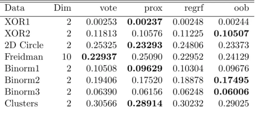
Table 3.6. Misclassification Error Rate N=1000
Data Dim vote prox regrf oob
XOR1 2 0.00253 0.00237 0.00248 0.00244 XOR2 2 0.11813 0.10576 0.11225 0.10507 2D Circle 2 0.25325 0.23293 0.24806 0.23373 Freidman 10 0.22937 0.25090 0.22952 0.24129 Binorm1 2 0.10508 0.09629 0.10304 0.09676 Binorm2 2 0.19406 0.17520 0.18878 0.17495 Binorm3 2 0.06390 0.06156 0.06248 0.06006 Clusters 2 0.30566 0.28914 0.30232 0.29025
16 measured by mean squared loss function. See chapter 5 for detailed conclusions.
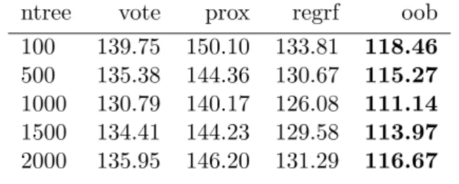
3.7.3 Normal Cluster Mixtures with Different Ntrees
We set N=500 as the sample size for training data set to build the tree. We also use the test data from 100 independent sample with sample size 1000 to evaluate the probability estimates. The final mean squared loss of the sample is the average of the losses for the 100 times’ simulations. So does the misclassification error rate.
Table 3.7. Mean Squared Loss for Normal Cluster Mixtures with Different Ntrees
ntree vote prox regrf oob
100 139.75 150.10 133.81 118.46
500 135.38 144.36 130.67 115.27
1000 130.79 140.17 126.08 111.14
1500 134.41 144.23 129.58 113.97
2000 135.95 146.20 131.29 116.67
Table 3.8. Misclassification Error Rate for Normal Cluster Mixtures with Different Ntrees
ntree vote prox regrf oob
100 0.32301 0.30157 0.31923 0.30653 500 0.18684 0.17452 0.18284 0.14952
1000 0.29892 0.28013 0.29689 0.28419 1500 0.3092 0.28997 0.30695 0.29367 2000 0.29299 0.27547 0.29019 0.27854
17 CHAPTER 4
DATA EXAMPLES 4.1 Brier Score
The Brier score is calculated by the original definition according to Wikipedia [13]. It is defined: BS = 1 N N X n=1 K X i=1 (fti−oti)2,
whereN is the number of cases andK is the number of the classes for the events. ftiis the estimated probability, oti is the actual outcome of the event at caset (0 if it doesn’t occur and 1 if it occurs). For binary response variables, there is an alternative definition, which would give results half as big as ours.
4.2 10-fold Cross Validation
Cross validation is a useful statistical technique to access the performance of a statistical model or algorithm. The general idea of cross validation is dividing the data into two parts: one is the training data set and is used to build the model; the other one is testing data set or validation set and is used to validate and evaluate the model.
10-fold cross validation is mostly commonly used in machine learning. The original data set is randomly separated into 10 subsets with equal sample size N/10. 1 subset is chosen as the testing set and the other 9 are the training sets. Each time we choose a different testing set and repeat the procedure 10 times, therefore all the observations are tested exactly once. The estimation is obtained by combining the results from each testing set. [12]
4.3 Missing Values
There are many ways to deal with missing values and we replace them in two ways:
4.3.1 Na.roughfix
Na.roughfix is an R function in the Random Forests package which replaces the NAs with column medians if the variables are numeric, or the most frequent levels if the variables
18 are categorical. [8]
4.3.2 RfImpute
There is another function to deal with missing data called “rfImpute” in the Random Forest R package. The algorithm starts by imputing NAs using na.roughfix. Then there aren’t any missing values in the data set and randomForest is used to obtain the proximity matrix, therefore updating the imputation of the NAs. For continuous variables, the im-puted value is the weighted average of the non-missing values, in which the weights are the proximities. For categorical variables, the imputed value is the category with the largest average proximity. The process is iterated 5 times. [7]
4.4 Results for Real Data
The methods are compared on 23 datasets from UCI Repository. We use 10-fold cross validation to estimate the Brier score for each data set.
We used ntree=500 for all the datasets. The regression method only works for a binary response variable, therefore, we put NAs in the tables when there are more than 2 classes.
19
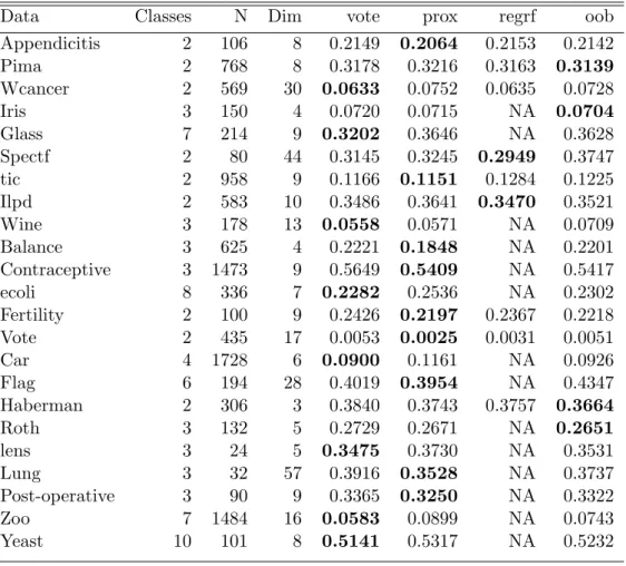
Table 4.1. Brier Score(Missing values are replaced using rfImpute)
Data Classes N Dim vote prox regrf oob
Appendicitis 2 106 8 0.2149 0.2064 0.2153 0.2142 Pima 2 768 8 0.3178 0.3216 0.3163 0.3139 Wcancer 2 569 30 0.0633 0.0752 0.0635 0.0728 Iris 3 150 4 0.0720 0.0715 NA 0.0704 Glass 7 214 9 0.3202 0.3646 NA 0.3628 Spectf 2 80 44 0.3145 0.3245 0.2949 0.3747 tic 2 958 9 0.1166 0.1151 0.1284 0.1225 Ilpd 2 583 10 0.3486 0.3641 0.3470 0.3521 Wine 3 178 13 0.0558 0.0571 NA 0.0709 Balance 3 625 4 0.2221 0.1848 NA 0.2201 Contraceptive 3 1473 9 0.5649 0.5409 NA 0.5417 ecoli 8 336 7 0.2282 0.2536 NA 0.2302 Fertility 2 100 9 0.2426 0.2197 0.2367 0.2218 Vote 2 435 17 0.0053 0.0025 0.0031 0.0051 Car 4 1728 6 0.0900 0.1161 NA 0.0926 Flag 6 194 28 0.4019 0.3954 NA 0.4347 Haberman 2 306 3 0.3840 0.3743 0.3757 0.3664 Roth 3 132 5 0.2729 0.2671 NA 0.2651 lens 3 24 5 0.3475 0.3730 NA 0.3531 Lung 3 32 57 0.3916 0.3528 NA 0.3737 Post-operative 3 90 9 0.3365 0.3250 NA 0.3322 Zoo 7 1484 16 0.0583 0.0899 NA 0.0743 Yeast 10 101 8 0.5141 0.5317 NA 0.5232
20
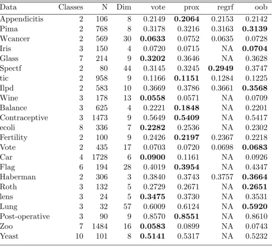
Table 4.2. Brier Score(Missing values are replaced using na.roughfix)
Data Classes N Dim vote prox regrf oob
Appendicitis 2 106 8 0.2149 0.2064 0.2153 0.2142 Pima 2 768 8 0.3178 0.3216 0.3163 0.3139 Wcancer 2 569 30 0.0633 0.0752 0.0635 0.0728 Iris 3 150 4 0.0720 0.0715 NA 0.0704 Glass 7 214 9 0.3202 0.3646 NA 0.3628 Spectf 2 80 44 0.3145 0.3245 0.2949 0.3747 tic 2 958 9 0.1166 0.1151 0.1284 0.1225 Ilpd 2 583 10 0.3669 0.3786 0.3661 0.3568 Wine 3 178 13 0.0558 0.0571 NA 0.0709 Balance 3 625 4 0.2221 0.1848 NA 0.2201 Contraceptive 3 1473 9 0.5649 0.5409 NA 0.5417 ecoli 8 336 7 0.2282 0.2536 NA 0.2302 Fertility 2 100 9 0.2426 0.2197 0.2367 0.2218 Vote 2 435 17 0.0703 0.0720 0.0698 0.0683 Car 4 1728 6 0.0900 0.1161 NA 0.0926 Flag 6 194 28 0.4019 0.3954 NA 0.4347 Haberman 2 306 3 0.3840 0.3743 0.3757 0.3664 Roth 3 132 5 0.2729 0.2671 NA 0.2651 lens 3 24 5 0.3475 0.3730 NA 0.3531 Lung 3 32 57 0.6009 0.6124 NA 0.5920 Post-operative 3 90 9 0.8570 0.8551 NA 0.8610 Zoo 7 1484 16 0.0583 0.0899 NA 0.0743 Yeast 10 101 8 0.5141 0.5317 NA 0.5232
21 CHAPTER 5
CONCLUSIONS
For the Simulations, sample sizes have some effects on the performance of each methods. For the third case of the bivariate normal model: when N = 100, vote gives the smallest mean squared loss; when N = 500, the regression method makes the mean squared loss smallest; when N = 1000, the proximity weighting method turns out to be the best. For the Freidman model, vote is the best probability estimation method when the sample size is 100 and 500, however, when the sample size increases to 1000, proximity weighting performs better.
Regardless of the sample size effects, the out-of-bag method performs better than other methods in XOR with 10% over lap, 2-dimensional circle model, two bivariate normal models and normal cluster mixtures. Proximity weighting does best in the XOR model without overlap. Proximity weighting does better than votes or regression in 2-dimensional circle model.
The misclassification error rate criterion gives a little different results: When N = 100 and 500, the out-of-bag method is slightly better than the proximity weighting method for XOR model without overlap; whenN = 500 and 1000, the proximity method gives smallest misclassification error rate instead of the out-of-bag method for 2-dimensional circle model and the Binorm1; The proximity weighting method performs best instead of the out-of-bag method for Binorm2 whenN = 100 and the normal cluster mixtures whenN = 1000.
Only considering the misclassification error rate measurement, the out-of-bag method gives the smallest misclassification error rate. However, when the sample size of training data set increases, the proximity method tends to be better. Both the two methods ap-parently perform better than other methods, however, either of them can beat the other consistently.
Testing all the methods on real datasets, however, no methods did consistently better than all other methods. When we replace missing values with the rfImpute method, prox-imity weighting does best in more data sets. When we replace missing values with the
22 na.roughfix method, among the three methods, vote, proximity weighting and oob, no one is consistently better than the others. However, the regression method doesn’t perform well when it is applicable, no matter what method we use to deal with missing data.
23 CHAPTER 6
DISCUSSION AND FUTURE WORK
The two new methods, proximity weighting and out-of-bag method, outperform the current methods in almost all the simulations. However, experimenting on the real data sets, the the out-of-bag method doesn’t perform as well as it performs in the simulations and proximity weighting isn’t significantly better than votes, based on the 23 data sets from the UCI machine learning repository. I would like to experiment on more data sets to have more confidence in the conclusions in the future.
In the simulations, sample size has very significant influence on the third case of the bivariate normal model according to mean squared loss measurement. I would like to further explore why this happens by doing more different simulations for the binorm model and thinking about it theoretically. Sample size has even more influence according to the misclassification error rate measurement, it is worthwhile to find out the reasons. Also I would like to figure out why proximity weighting performs better than the out-of bag method in XOR model without overlap. The 10-dimensional model is another simulation I would like to do more theoretical research on to figure out why the out-of-bag method performs so bad on this model.
The current version of the code for the out-of-bag method only works for numeric pre-dictors, we have to convert the non-numeric predictors into numeric ones. Hence, we would like to improve the code for categorical predictors.
One interesting feature of the real data comparisons is that the missing value imputation method makes such a big difference.
24 REFERENCES
[1] L. Breiman,Random forests, Machine Learning, 45 (2001), pp. 5–32.
[2] A. Cutler, D. R. Cutler, and J. R. Stevens,Tree Based Methods, High-Dimensional Data Analysis in Cancer Research, Springer, New York, 2009.
[3] D. Eddelbuettel and R. Francois,Rcpp: Seamless r and c++ integration,
http://-cran.r-project.org/web/packages/Rcpp/index.html, (2013).
[4] J. H. Friedman, On bias, variance, 0/1-loss, and the curse-of-dimensionality, Data Mining and Knowledge Discovery, 1 (1997), p. 5577.
[5] T. Hastie, R. Tibshirani, and J. Friedman, The Elements of Statistical Learning,
Springer, New York, 2009.
[6] T. H. J. Friedman and R. Tibshirani, Additive logistic regression: a statistical view of boosting, Annals of Statistics, 28 (2000), p. 337374.
[7] A. Liaw, Missing value imputations by randomforest, http://rss.acs.unt.edu/Rdoc/
library/randomForest/html/rfImpute.html.
[8] , Rough imputation of missing values, http://rss.acs.unt.edu/Rdoc/library/-randomForest/html/na.roughfix.html.
[9] ,randomforest: Breiman and cutler’s random forests for classification and regression, http://cran.r-project.org/web/packages/randomForest/index.html, (2012).
[10] J. D. Malley, J. Kruppa, A. Dasgupta, K. G. Malley, and A. Ziegler, Proba-bility machines: Consistent probaProba-bility estimation using nonparametric learning ma-chines, Methods Inf Med, 51(1) (2012), p. 7481.
[11] D. Mease, A. J. Wyner, and A. Buja,Boosted classification trees and class probabil-ity/quantile estimation, Journal of Machine Learning Research, 8 (2007), pp. 409–439.
25 [12] P. Refaeilzadeh, L. Tang, and H. Liu,Crossvalidation,http://www.cse.iitb.ac.in/
-∼tarung/smt/papers ppt/encycrossvalidation.pdf, (2008).