Performance of Latent Dirichlet Allocation with Different Topic and Document Structures

(1)

Clemson University

TigerPrints

All Dissertations

Dissertations

8-2019

Performance of Latent Dirichlet Allocation with Different Topic

and Document Structures

Haotian Feng

Clemson University, [email protected]

Follow this and additional works at: https://tigerprints.clemson.edu/all_dissertations

Recommended Citation

Feng, Haotian, "Performance of Latent Dirichlet Allocation with Different Topic and Document Structures" (2019). All Dissertations. 2448.

https://tigerprints.clemson.edu/all_dissertations/2448

This Dissertation is brought to you for free and open access by the Dissertations at TigerPrints. It has been accepted for inclusion in All Dissertations by an authorized administrator of TigerPrints. For more information, please contact [email protected].

(2)

Performance of Latent Dirichlet Allocation with

different topic and document structures

A Dissertation Presented to the Graduate School of

Clemson University

In Partial Fulfillment of the Requirements for the Degree

Doctor of Philosophy Statistics by Haotian Feng August 2019 Accepted by:

Dr. William Bridges, Committee Chair Dr. Alexander Herzog

Dr. Jun Luo Dr. Christopher McMahan

(3)

Abstract

Topic modeling has been used widely to extract the structures (topics) in a collection (cor-pus) of documents. One popular methods is Latent Dirichlet Allocation (LDA). LDA assumes a Bayesian generative model with multinomial distributions of topics and vocabularies within the top-ics. The LDA model result (i.e., the number and types of topics in the corpus) depends on tuning parameters. Several methods, ad hoc or heuristic, have been proposed and analyzed for selecting these parameters. But all these methods have been developed using one or more real corpora. Un-fortunately, with real corpora, the true number and types of topics are unknown and it is difficult to assess how well the data follow the assumptions of LDA. To address this issue, we developed a factorial simulation design to create corpora with known structure that varied on the following four factors: 1) number of topics, 2) proportions of topics in documents, 3) size of the vocabulary in topics, and 4) proportion of vocabulary that is contained in documents. Results suggest that the quality of LDA fitting depends on the document-topic distribution and the fitting performs the best when the document lengths are at least four times the vocabulary size. We have also proposed a pre-processing method that may be used to increase quality of the LDA result in some of the worst-case scenarios from the factorial simulation study.

(4)

Dedication

To my mother and father, Yan Ma and Jianping Feng. To my wife, Zhuhua Tang. To my dear little son, Huaiyuan Feng.

(5)

Acknowledgments

First and foremost, I would like to thank my advisor Dr. William Bridges for his constant support, patience and guidance throughout my doctoral studies. Billy, thank you for being an invaluable source of wisdom and ideas and more importantly for being a role model of a researcher and a teacher. This is the only section that you can not edit and please be calm when you find any bad sentences.

I am thankful to my committee members Dr. Alexander Herzog, Dr. Jun Luo, Dr. Christo-pher McMahan, and Dr. Ilya Safro for their helpful and insightful comments and opinions that made this dissertation better.

I would like to mention those who have made the journey through my doctoral studies an exciting and enjoyable experience. I would like to start by thanking Dr. Scott R Templeton and Dr. Christopher Cox for their support in helping me switching from Economics major to Math major. Many thanks for the instruction and guidance from Dr. Kevin James and Dr. Taufiquar Khan, who has provided a wonderful environment in the mathematics department.

Lastly, I would like to thank my family. Jianping Feng and Yan Ma, it is your endless love and encouragement that makes me be myself now. Zhuhua Tang, my dear wife, flew thousands miles away from home to accompany me in the other side of the planet. Huaiyuan V. Feng, my son little Varian, took all my spare time and are planning to do the same in the future. I can’t imagine being able to complete my doctoral studies without the unconditional support from my family.

(6)

List of Tables

1.1 Sample Data from the Collection of the Selected Books . . . 4

1.2 Contingency table and Evaluation metrics generated from it . . . 8

1.3 Common similarity measurements used in measuring distance between probability distributions . . . 9

1.4 Categories of Evaluation . . . 9

3.1 Pilot Study Fitted Topic-word distributions . . . 50

3.2 Pilot Study Fitted Document-topic distributions . . . 51

3.3 Pilot Study result Summary . . . 53

3.4 Matching Fitted topic with True topic by rank . . . 54

3.5 Pilot Study Correlation Coefficient for topic matching . . . 57

3.6 Pilot Study Correlation Coefficient Topic Matching Rep . . . 58

4.1 Basic information about the selected Corpus . . . 62

4.2 Sample Corpus Basic Descriptive Statistics of the Document Length Ratio . . . 65

4.3 Mean size of vocabulary of sample size 100 . . . 74

5.1 Comparing the Mean and the Standard Deviation of the Correlations between Fitted and True Topics for LDA using the Dirichlet Prior and LDA using the Multi-normal Prior . . . 117

5.2 Comparing the Min and the Max of the Correlations between Fitted and True Topics for LDA using the Dirichlet Prior and LDA using the Multi-normal Prior . . . 120

5.3 Summary Descriptive Statistics for Each Level of Document Length Ratio with Dirich-let prior . . . 131

5.4 Summary Descriptive Statistics for Each Level of Document Length Ratio with Multi-normal prior . . . 132

5.5 Summary of the Estimated regression coefficients of the simple linear regression model for Size of Vocabulary analysis . . . 133

5.6 Summary Descriptive Statistics for Categories of Size of Vocabulary with Dirichlet prior133 5.7 Summary Descriptive Statistics for Categories of Size of Vocabulary with Multi-normal prior . . . 134

5.8 Average Correlation for Extreme Cases . . . 137

5.9 Average Correlation for Mixture Cases . . . 137

5.10 Average Correlation for Analytical Mixture Cases, First group . . . 137

5.11 Average Correlation Differences for Analytical Mixture Cases, First group . . . 138

5.12 Average Correlation for Analytical Mixture Cases, Second group . . . 138

5.13 Compare Case 1 and Case 2 Mean Correlations for different Document Length Ratio 140 5.14 Parameter Selection for Pre-processing Corpus Construction . . . 141

5.15 Correlations between the True Topics and Fitted LDA Topics for the Original Corpus 141 5.16 Correlations between the True Topics and Fitted LDA Topics for the Corpus with Additional Document . . . 143

(8)

List of Figures

1.1 Topic illustration . . . 2

1.2 Topic-word distribution generated by Latent Dirichlet Allocation . . . 5

1.3 Example of multinomial distribution samples drawn from Dirichlet distributions with different parameterα. . . 13

2.1 Example of Document-Topic distribution for 2 documents and 5 Topics . . . 19

2.2 A Venn Diagram illustrating the probability that both event happen. Areas represent probabilities . . . 20

2.3 Layer of Texts . . . 22

2.4 Unrolled graphical model representation of LDA . . . 30

2.5 The Graphical model representation of the variation EM algorithm . . . 35

3.1 Venn’s Diagram of the relationship between Language Models and Topic Models . . 41

3.2 Topic-word distribution of Pilot Study . . . 45

3.3 Document-topic distribution of Pilot Study . . . 46

3.4 Pilot Study Fitted Topic-word distributions . . . 50

3.5 Pilot Study Fitted Document-topic distributions . . . 51

3.6 Rank plot of Pilot Study Fitted Topics . . . 54

3.7 Match Topics by percentage of rank-matching . . . 55

3.8 Match Topics by percentage of rank-matching - Level Selection . . . 56

4.1 Structure of Simulations . . . 61

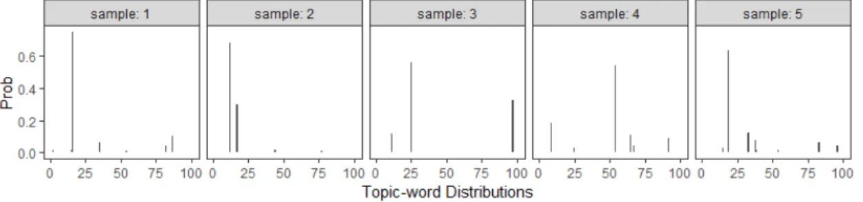
4.2 Five samples of Topic-word distributions generated from Dirichlet prior that has con-centration paramter 0.01 . . . 64

4.3 Document Length Ratio of Reuters21578 Data . . . 66

4.4 Document Length Ratio of 20 Newsgroups Data . . . 67

4.5 Document Length Ratio of Associated Press Data . . . 68

4.6 Document Length Ratio of aclIMDB Data . . . 69

4.7 Simulated Analysis of Document length ratio for Dirichlet prior . . . 71

4.8 Simulated Analysis of Document length ratio for Multi-normal prior . . . 72

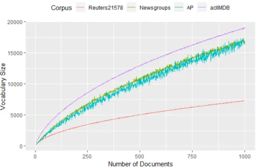
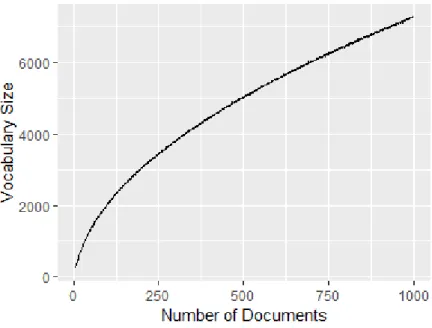
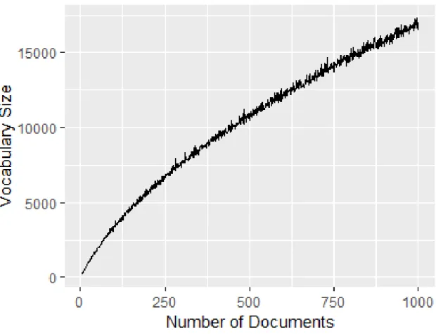
4.9 Vocabulary Size changes based on the Number of Documents for Four different Corpus 73 4.10 Plot of Number of documents vs Vocabulary size for sample size 100, from 5 to 1000, data set Reuters21578 . . . 75

4.11 Plot of Square root of Number of documents vs Vocabulary size for sample size 100, from 5 to 1000, data set Reuters21578 . . . 75

4.12 Residual Plot for Reuters21578 data . . . 76

4.13 Regression Line with Reuters 21578 Data Set . . . 77

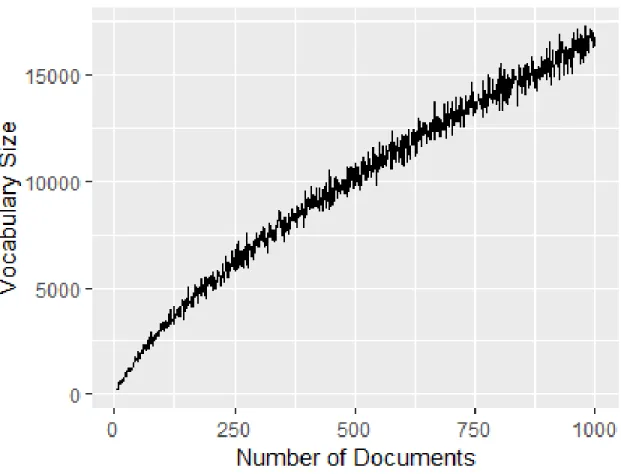
4.14 Plot of Number of documents vs Vocabulary size for sample size 100, from 5 to 1000, data set 20 Newsgroups . . . 78

4.15 Residual Plot for 20 Newsgroups data . . . 79

(9)

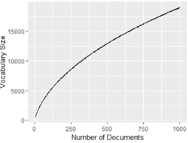
4.17 Plot of Number of documents vs Vocabulary size for sample size 100, from 5 to 1000,

data set Associated Press . . . 81

4.18 Residual Plot for 20 Associated Press data . . . 82

4.19 Regression Line with Associated Press Data Set . . . 83

4.20 Plot of Number of documents vs Vocabulary size for sample size 100, from 5 to 1000, data set aclIMDB . . . 84

4.21 Residual Plot for 20 aclIMDB data . . . 85

4.22 Regression Line with aclIMDB Data Set . . . 86

4.23 Simulated Analysis of Size of Vocabulary for Dirichlet prior . . . 88

4.24 Simulated Analysis of Size of Vocabulary for Multi-normal prior . . . 88

4.25 Correlation between true and fitted topics with varying document length ratio for Case 1 . . . 91

4.26 Correlation between true and fitted topics with varying size of vocabulary for Case 1 92 4.27 Correlation between true and fitted topics with varying document length ratio for Case 2 . . . 93

4.48 Correlation between true and fitted topics with varying size of vocabulary for Case 12 112 5.1 Approximate Density of the Difference between Means of Correlations . . . 116

5.2 Approximate Density of the Difference between Standard Deviations of Correlations 118 5.3 The Regression Plot of the Mean Correlation vs logarithm of the Document Length Ratio, Dirichlet prior . . . 121

(10)

5.4 The Regression Plot of the Mean Correlation vs logarithm of the Document Length Ratio, Multi-normal prior . . . 122 5.5 The Regression Plot of the Standard Deviation of Correlation vs logarithm of the

Document Length Ratio, Dirichlet prior . . . 124 5.6 The Regression Plot of the Standard Deviation of Correlation vs logarithm of the

Document Length Ratio, Multi-normal prior . . . 125 5.7 The Regression Plot of the Minimum of Correlation vs logarithm of the Document

Length Ratio, Dirichlet prior . . . 127 5.8 The Regression Plot of the Minimum of Correlation vs logarithm of the Document

Length Ratio, Multi-normal prior . . . 128 5.9 The Regression Plot of the Maximum of Correlation vs logarithm of the Document

Length Ratio, Dirichlet prior . . . 129 5.10 The Regression Plot of the Maximum of Correlation vs logarithm of the Document

Length Ratio, Multi-normal prior . . . 130 5.11 Size of Vocabulary vs Correlations between the True topic and Fitted Topic, Dirichlet

Prior . . . 134 5.12 Size of Vocabulary vs Correlations between the True topic and Fitted Topic,

Multi-normal Prior . . . 135 5.13 Heatmap Summary of Document Length Ratio Simulation Results . . . 136 5.14 Heatmap Summary of Size of Vocabulary Simulation Results . . . 136 5.15 Correlation Structure of the True and Fitted Topic-word Distributions without the

pre-processing step . . . 142 5.16 Correlation Results for Different Document Length of the Added Document . . . 144

(11)

Chapter 1

Introduction

1.1

Motivation

In linguistics, the concept of “topic” was originally described as the item that the sentence is about. When extended to the whole document, the concept of “topic” evolved towards “abstract”, which usually consists of a few sentences. In an abstract, information is concentrated and com-municated while details are omitted. This allow readers to quickly decided if they have interest in the document. Readers save valuable time and can focus on articles of interest. As the number of documents has increased, keywords/labelling systems begin to be important because even reading abstracts became too time consuming.

As far back as the of year 1800, around the time that Joseph Marie Jacquard invented the Jacquard loom, human beings started to convert natural language to something that a machine could record. In 1945, the earliest electronic general-purpose computer called Electronic Numerical Integrator And Computer (ENIAC) was completed. It didn’t take too long before people realized that computers were more efficient than human beings for recording and summarizing documents. In 1950, Calvin Moores formally defined the term “Information Retrieval”[23] as the discovery and location of stored-away information so that it can be used. He specifically pointed out the difference between Information Retrieval and Information Warehousing. The later is more like the database systems we are using today for cataloging and storage of information. The simplest method to do information retrieval is to carefully describe the information wanted in terms of a natural language description and then search the whole database to find documents that match the description. There

(12)

Figure 1.1: Topic illustration

are two main problems with this simple method of information retrieval:

• Human beings often can not accurately describe everything they want in terms of natural language.

• The complexity of linguistics allow several possible descriptions that are essentially equivalent to each other.

To solve these problems, researchers started to use sets of keywords instead of a natural language description to conduct information retrieval. Hence, for each information retrieval inquiry, we can just return the set of articles that contain the same set of keywords or a related set of keywords. In 1955, James W. Perry introduced “precision” and “recall” as concepts to evaluate the quality of an information retrieval task[24]. This was the start of systematic and objective evaluations of information retrieval tasks.

Topic modeling is a specific method of information retrieval that uses statistical tools to discover the ”Topics” that occur in a collection of articles. “Topic” is defined as a multinomial distribution over the words in a vocabulary. Consider a simulated document with a vocabulary consisting of six words: elephant, lion, tiger, logistic, sampling, stochastic. Human beings would most likely recognize two potential sets within the vocabulary and we would probably name them

(13)

“animals” and “statistics”. Instead of giving a name to each set of words, topic modeling treats these two sets as two probability distributions. Figure 1.1 shows an illustration of the two topic distributions in a simulated document. Two interesting observations from Figure 1.1 are:

1. The probabilities for words like elephant are very small within topic 1, but are not zero. This can be interpreted as it is very rare but possible that someone has document about a statistical experiment related to elephants (or some combination like this)

2. The sets of words that have relatively high probabilities represent the original concept of ”Topic” as we discussed above. We will use topic-distribution or topic-word distribution for clarity in the remainder of this dissertation.

With the help of computers, searching and discovering relevant pieces of information has evolved from supervised methodologies to unsupervised methodologies. By saying unsupervised, it means that the methods will produce results without the need of assistance from humans, but only after the data has been properly processed and the parameter estimates have been selected. Topic models are considered some unsupervised but do require participation of human beings during the processing. Statistical topic modeling is a useful method for finding topics in large unstructured document collections. Typical applications of topic modeling includes document clustering[31], ex-ploratory data analysis and visualization[30], retrieving document translation pairs[21], and auto-matic labelling[20].

One of the most widely used topic model methodologies is Latent Dirichlet Allocation (LDA) [4]. It allows multiple topics which are represented by multinomial topic-word distributions for one document and documents may possess different topic structures which are represented by the document-topic distribution. A Bayesian estimation approach allows the LDA model the flexibility of extension and makes the estimation steps easier. Documents may possess different topic structures and topics may evolve as new data are observed. More details of LDA are going to be discussed in Chapter 2.

While the LDA methodology is widely used to produce an estimated topic-word distribu-tions, there is no guarantee that the resulting set of topics is correct. In fact, the concept of the correct set of topics is not well understood in topic modeling. Some previous work has been done on evaluating topic modeling results, but they do not directly address the issue of the correct set of topics.

(14)

document word n Deathly Hallows 33 snape 113

Goblet Fire 36 dumbledore 95 Deathly Hallows 10 kreacher 87 Goblet Fire 21 dobby 77 Goblet Fire 30 dumbledore 76 Chamber Secrets 2 dobby 65 Deathly Hallows 35 dumbledore 63 Goblet Fire 24 hagrid 63 Deathly Hallows 23 greyback 61 Deathly Hallows 24 wand 61 Goblet Fire 27 sirius 61

Table 1.1: Sample Data from the Collection of the Selected Books

Developing techniques to determine if the topics produced by topic modeling are correct is the primary objective of this research. In the next section the current methods of evaluating topic modeling results will be discussed; but first an example illustrating the concept of correct topics will be discussed. Suppose we are trying to find the topics for a collection of three randomly selected

Harry Potter books : Chamber of Secrets,Deathly Hallows, andGoblet of Fire. Since there are three books, we set the number of topics to be detected as three and use the standard default R package

topicmodels. After removing the default stop-words (words that are considered meaningless, i.e. “a”, “the”) intopicmodelsand applying the proper pre-processing steps, the three books are then converted to a data set that suitable for LDA analysis. Table 1.1 shows part of the data set.

The resulting of the three fitted topic-word distributions are shown in Figure 1.2. This is clearly not the correct set of topics based on simple observation of the plots without the need of any formal statistical analysis. Some of the issues that indicate that this particular LDA solution is not the correct set of topics include:

• ”harry” is the highest frequency word within each topic distribution.

• Names in general appear too often as high frequency words in the distributions.

• Topic 1 and Topic 3 of the LDA solution have the same five words with the highest distributions. A solution to finding the correct topic distributions in this specific example is straightforward. One can simply eliminated all the formal names from the data set to remove them in the LDA solution. But to figure out what names should be removed, one needs to read the text thoroughly and that is out of the scope of an un-supervised method like LDA and requires even more assistance from human

(15)

Figure 1.2: Topic-word distribution generated by Latent Dirichlet Allocation

beings. In this dissertation, we will present a method that systematically evaluates the performance of LDA model under different scenarios.

It is worth noting that topic models are applied on data sets from unstructured texts. However, topic model methods usually explicitly or implicitly assume a structure for the texts from which the data sets are developed. In Chapter 3 we will discuss more about the structures implicitly and explicitly proposed by LDA methodology.

1.2

Previous Research on Topic Model Evaluation

The evaluation methods can be divided into four categories. The categories are combinations of two classification factors. The first classification factor is intrinsic vs extrinsic and the second classification factor is efficient vs accurate.

1.2.1

Intrinsic vs. Extrinsic

The intrinsic vs extrinsic classification is based on whether or not extra tasks are required to perform the evaluation. Intrinsic evaluations only consider the fitted result and the original data set. On the other hand, extrinsic evaluations utilize extra tasks which take the topic model outputs (i.e. topic-word distributions) and evaluate the quality of the topic model with based on the extra tasks.

(16)

1.2.2

Efficiency vs Accuracy

The efficient vs accurate classification is based on whether or not the metric used in the evaluation depends on the situation. Efficiency measures the time and resources required for the method to produce results and independent to the method itself. Accurate measures how well the model performs based on the selected scenario. Efficiency has a clear definition and usually consists of time complexity and memory usage which are discussed in detail below. Accuracy, on the other hand, is still struggling in finding a good measure. Table 1.4 illustrates the categories for evaluation methods. It is worth noting that the two types of evaluation methods are related to each other and may be used as trade-off pairs.

In general, efficiency is easy to measure and accuracy is much more difficult to measure.

1.2.2.1 Efficiency

There are usually two methods of measuring efficiency. The first method is based on the computational complexity to process the model, and this method is part of the intrinsic evalua-tion. The second method is based on the time or resource consumed to process the model in real applications and this method is part of extrinsic evaluation.

The computational complexity not only depends on the structure of the model itself, but also depends on the procedures used for estimating the model parameters. For LDA, the original paper [4] derived an estimation algorithm that uses variational inference but in [12], a bayesian approach usingthe Gibbs Sampling procedure is developed for estimation. So there are usually multiple estimation methods that can be selected for a given model. In addition to the multiple estimation techniques, many topic models are designed to enhance the performance under specific scenarios and use extra information besides the dataset. For these reasons (multiple estimation techniques and specific scenarios), computational complexity is rarely used as a measure of efficiency. However, if a standard data set and standard estimation algorithm were chosen for testing topic models, this might change in the future.

Extrinsic measurement of efficiency is based on time and resource used to completely process the model. For this method of efficiency, there are some widely used standard data sets. These data sets are considered as the ”standard” data sets, and the time and resource consumed to perform the same task may be used to compare topic model approaches. The sizes of data sets have increased

(17)

rapidly due to internet searching and new tools had been developed to reduce the time and resources required for these large data sets. For example, Gropp et al.[13] derived Clustered Latent Dirichlet Allocation and showed that the model does well in terms of the wall-time when the number of processors is increased. The quality of the result in terms of perplexity (to be discussed later) is not degenerated. In the same paper, they also proved that the CLDA model conserves the ability of expansion from simple LDA model.

Since standard data sets do exists, extrinsic efficiency evaluations are straight forward to check, easy to compare, and have little ambiguity. But the measure of efficiency is partly determined by the physical configuration of the platform which researcher is using. The same algorithm may have different running time on different computers. Hence, comparing the efficiency measurements across papers is hard, if not impossible. As a result, there does not exist a preferred system of efficiency evaluation.

1.2.2.2 Accuracy

The accuracy evaluation approach is based on trying to determine how accurately the true underlying topics are discovered by the topic model. The term “Accuracy” is commonly used within the area of statistics and has several definitions. Table 1.2 lists the definitions of Accuracy and several related measures based on a confusion matrix. These metrics are all designed to determine (in slightly different ways) if the model is performing “accurately” for the given task. The problem with using theses “accuracy” measures from a confusion matrix is the requirement of a “True Condition” which is rarely known in topic modeling. Also, topics models require both the topic-word distribution and the document-topic distribution to be estimated, so there are actually two levels of “True Condition”. Hence, the definitions of “accuracy” from Table 1.2 can’t be directly applied.

1.2.2.3 Perplexity and Other Intrinsic Measurements

Perplexity is one of the most widely used intrinsic methods to evaluate topic models. It was originally introduced in information theory as a measure of how well a probability distribution predicts a sample. It is based on the log-likelihood of the language model, which tries to predict the next word given the current word. For example, suppose there is a documentDthat is written under topicT. Under topic model assumptions, the documentDis equivalent with a list of frequencies of the words which showed up, and the topicT is a probability distribution over the whole vocabulary.

(18)

True Condition

Total

popu-lation Condition positive Condition negative

Predicted condition

condition

positive True positive False positive

condition

negative False negative True negative

P_{True positive}

P_{Condition positive}, True positive

rate (TPR), Recall, Sensitivity, probability of detection

P_{False positiv}

P_{Condition negative},False positive

rate (FPR), Fall-out

P_{False negative}

P_{Condition positive},False negative

rate (FNR), Miss rate

P_{True negative}

P_{Condition negative}Specificity

(SPC), Selectivity, True negative rate (TNR)

P_{Condition positive}

P_{Total populatio} ,Prevalence

P_{True positive+}P_{True negative} P_{Total population} ,

Ac-curacy (ACC)

P_{True positive}

P_{Predicted condition positive},Positive

predictive value (PPV), Preci-sion

P_{False positive}

P_{Predicted condition positive},False

discovery rate (FDR)

P_{False negative}

P_{Predicted condition negative},False

omission rate (FOR)

P_{True negative}

P_{Predicted condition negative},

Neg-ative predictive value (NPV)

T P R

F P R,Positive likelihood ratio

(LR+)

LR+

LR−, Diagnostic odds ratio

(DOR)

F N R

T N R,Negative likelihood ratio

(LR)

(19)

Similarity Metric Algebraic Expression Min. Value Max. Value Kullback-Liebler (KL) Pn i=1p(xi)logp_q₍(x_xi) i) 0 ∞ Jensen-Shannon (JS) 1 2KL(p, p+q 2 ) + 1 2KL(q, p+q 2 ) 0 1 Hellinger (He) Pn i=1( p p(xi)− p q(xi))2 0 2

pand qare two discrete probability distributions

Table 1.3: Common similarity measurements used in measuring distance between probability distri-butions

Efficient Accurate Intrinsic Run time for one specific model Perplexity

Extrinsic Memory consumption for Accuracy in Retrieve Parallelized computing documents under a specific topic

Table 1.4: Categories of Evaluation

The likelihood is the probability that the documentDis presented as it is now under the probability distributionT. The log-likelihood is the log transformation of the likelihood to avoid the extremely small value.

Similarly, the ideas of information entropy (the expectation of the negative log likelihood) is trying to quantify the uncertainty of texts, the Kullback-Leibler divergence (Table 1.3) measures the distance between two probability distributions that is not symmetric, the Jensen-Shannon divergence and Hellinger divergence measure the symmetric distance between two distributions. They are some of the classical metrics inherited from information theory. Manning [5] showed how perplexity is generated from entropy. Hanna Wallach in [28] showed in detail on how to estimate perplexity.

1.2.2.4 Human Interpretability

Topic models have the potential to provide a better understanding of large document col-lections by discovering interpretable topics (or small sets of words). This process may be viewed as a type of dimension reduction. One way to measure the quality of the model results is to ask human experts to review the topics that been produced and comment the accuracy of how the model topics reflect the true underlying topics in the documents. Unfortunately, it is often the case that the data set based on the collection of documents is too large or too diverse for any human to accomplish this task.

(20)

1.2.2.5 Other Ad-hoc Measurements

For a specific task, often an ad-hoc measurement of accuracy is created. A specific example comes from speech recognition tasks. Word-error rate and M-ref [8] has been shown to be better than perplexity in measuring accuracy.

1.3

Problems with the Current Evaluation Methods

1.3.1

Lack of truth or “true condition”

The lack of knowledge of the actual true underlying topics is the major problem for current evaluation methods. As an example, the two metrics precision and recall defined in Table 1.2 are widely used but they both require the knowledge about “True Positive” which is not available in general. In topic modeling, we may never know the true condition. Two experts may agree on the top few words which reflect the topic for a given article, however, when extended to 50 words, they most likely will diverge. It is also an unknown as to how many words from the word distribution should be included to find the best representation of a topic.

1.3.2

Issues with Perplexity

Perplexity is designed to measure the log-likelihood of a held-out test set. This is usually done by splitting the data set into two parts, one for training and the other for testing (the held-out part). A training set is used to estimate the document-topic distribution and the topic-word distribution. The held-out part, the test set, is then used to compute the perplexity value.

Suppose LDA model generates the document-topic distribution Θ and the topic-word dis-tribution Φ. The log-likelihood of the test set is

L(Dtest) = logP(Dtest|Θ,Φ) =

X

i

logP(Di|Θ,Φ)

The perplexity is then defined as

perplexity(Dtest) = exp{−

L(Dtest)

(21)

whereN is the total number of words in the test set andDi is the i-th document in the test set of

documents.

Perplexity provides an intrinsic evaluation measure, but it has several drawbacks. The first drawback was shown by Chen[8]. The issue was that, surprisingly, predictive likelihood (perplexity) and human judgement are often not correlated, and even sometimes slightly negatively correlated. They ran a large scale experiment on the Amazon Mechanical Turk platform. For each topic, they took the top five words of that topic and added a random sixth word (de). Then, they presented these lists of six words to participants asking them to identify the intruder word.

If every participant could identify the intruder, then we could conclude that the topic is well defined and easy to recognize. If on the other hand, many people identified one of the top five words from the topic as the intruder, it means that they could not easily identify the topic, and we can conclude the topic was not well defined. The result suggests that, given a topic, the five words that have the largest frequency within their topic are usually not enough to clearly describe a topic. A second issue with perplexity occurs when using modern Bayesian topic models with a more complicated structures of topics. These models often lead to an intractable posterior likelihood. For a held-out collection of test set Dtest documents and a corpus wide vocabulary ofV words, when

evaluating LDA model, perplexity is computed using the following formula:

perplexity(Dtest) = 2 {− PDtestlog( PNd n=1 PT t=1 (θdtφtn)) d=1 PDtest d=1 Nd }

where φtn is the inferred probability of word n in topic t and θdt is the probability of assigned

topic t to the held-out documentdwhile Nd is the total number of words in that document. The

multiplication ofθdtφtnis the part that is intractable. Since wordnmight be presented in multiple

topics, one needs to figure out which topic it belongs to at every time the wordnis presented, which is impossible.

Hence the perplexity has to be estimated through some sampling methods. In this situation, the estimated perplexity is not a deterministic measurement, but rather a stochastic measurement. This means that each time perplexity is estimated for the same corpus, the perplexity scores will be different.

The final draw-back for perplexity is shown in another word intrusion experiment conduct by Chang et al. [7]. In this paper, Chang et al. showed that the words in topics generated through

(22)

the lowest perplexity criteria often do not have natural semantic relationship with each other.

1.3.3

Model Assumptions

One big problem for topic models is that the model assumptions are not able to be validated. Some of the assumptions, like “Topics evolve in time so they are correlated to each other”, might be validated through a thorough investigation of the corpus. For a given corpus, one may find human experts to summarise the topics for each time period and compare the result. Methods to assess other assumptions, like “Topics are multinomial distribution over the vocabulary”, have not been developed.

1.3.4

Parameter Tuning

Simple models like the n-grams topic model which will be introduced in Chapter 2 do not have a parameter to be tuned. More complicated models such as Bayesian methods require selection of proper tuning parameters. Even the commonly used LDA model contains three parameters that need to be tuned. The standard tuning parameter selection method is to run the topic modeling approach several times over different setups of the parameter, and select the set of parameter values that produces the lowest perplexity score. When no parameter values produce a topic modeling result with a reasonable perplexity value, the topic modeling result does not make semantic sense, or the perplexity score varies widely based on the parameter values, there is no recommended alternative plan for parameter value selection.

The importance of the parameter tuning can not be over stated. In the LDA modeling approach, there is a parameterαthat defines the convergence rate and it plays an important role in the LDA results as illustrated in Figure 1.3. This figure shows how the associated document-topic multinomial distribution is going to change when the different value of the parameterαis used. A small α value leads to a multinomial distribution that contains few high-probability topics and a largeαvalue leads to a more “flat” multinomial distribution. The number of topics to be fitted is another important tuning parameter to be considered. Unlikeαthat can be interpreted as a prior belief, and this prior might be overridden in Gibbs Sampling process, the number of topics is the primary factor in evaluating the quality of modeling result.

(23)

Figure 1.3: Example of multinomial distribution samples drawn from Dirichlet distributions with different parameterα

(24)

1.3.5

Dependency of evaluation on a Particular Corpus

Although there are many articles produced each year, only a few are used for evaluation purpose. TREC (Text REtriveal Conference) publishes about 10 datasets a year, and approximately 1 human-annotated dataset for every 3 years. While these can be used as standards, the quality of the annotation is actually unknown and the annotated data may not be similar to other data sets used by researchers. The other reason that the evaluation method is corpus dependent is that some models require more information about the dataset than others. Rosen-Zvi et al. in [26] published a well-designed author-topic model for authors and documents. Without the certain type of information, the model should be at most has a similar quality as LDA.

1.3.6

Pre-processing Steps Impact on Evaluations

This is best illustrated in Figure 1.2. It is hard for anyone to get enough information about the topics from the graphs. There are all the names from the novel that take the higher probability. Should we remove the names if we know it is not helping? It is still not clear. The books are definitely talking about Harry Potter and his mates. Remove those names result in other “not-as-important” names showing up. For this specific example, maybe more topics or a longer list of words will help. But the pre-processing steps like stop-words recognition and tokenization do have influence on the topic model fitting result, but this has rarely been evaluated.

1.4

Build the Underline Truth

The generative process used in Bayesian Topic modeling provides a useful tool for correctly evaluating the model results. The main problem of not knowing the true condition is solved. Based on a carefully designed simulation, one can construct a corpus with known topic-word distribution as well as the document-topic distribution. In this case, We may also modify the assumptions from the model to check the performance of the model under different conditions. Knowing the true distributions also allow us to use the statistic measurements of agreement like correlation. It is also an attempt to avoid corpus dependency and issues associated with pre-processing steps. Parameter tuning might be studied in detail as well. We will talk about these in detail in Chapter 4.

(25)

We propose in this study to develop method to perform a proper evaluation.

In Chapter 2, we will develop the technical details in some classic topic models and evaluation methods. In Chapter 3, we will decompose the structure of LDA model and detect important characteristics. In Chapter 4, we will go through the detail of simulation study that can be used to evaluate topic model results. In Chapter 5, we will discuss the findings and future work.

The objective of this study is to learn the impacts of different topic and document structures to the performance of LDA model. The topic and document structures can be summarised with certain characteristics that will be discussed in Chapter 3. We would like to identify the impacts of different characteristics on topic modeling results.

(26)

Chapter 2

Technical Background

2.1

Introduction

In chapter 1 we briefly discussed Latent Dirichlet Allocation. In general, topic models are trying to extract article features, and use the features to represent articles for applications like answering a query. For these applications, the human interpretability is not always the largest concern. The techniques for extracting features are usually conducted within single articles first, and then extended to multiple documents. This extension to multiple articles is not an easy or simple extension and will be discussed later.

The simplest topic modeling approach is the unigram model. Word counts are used to summarize the information in the articles. The idea is simple: if a wordwoccurs more times than other words, thenwshould be able to capture more information compared with other words. ATopic, also known as theTopic-word distribution, is a multinomial distribution that assigns probability to each word in the vocabulary. Usually, a topic is illustrated by a few high-probability words. It is a natural extension of the idea of word counts. A collection of articles may contain multiple topics, denoted byK. Since a multinomial distribution can be represented by its parameter~p, it is sufficient to use the associated parameters to represent topics. Under this idea, multiple topics can be represented in a matrix: let ϕk = (p1, ..., pV), k = 1, ..., K be one set of parameters among K

topics, thenΦ={ϕk as row k,k= 1, ..., K} is the desired topic matrix.

The ultimate target of any Topic model is to find the properΦ, topic-word distribution, for any given collection of documents. We will discuss some basic definitions and terms first, then some

(27)

important probability background, and finish the chapter with formal details about topic models and evaluation methods.

2.1.1

Definitions and Terminology

In this section we will state clear definitions and terms for the discussion that follow. Some of the definitions and terms are quite self-explanatory, but we will try to provide a strict concepts instead of general ideas.

• Corpus: Corpus is a collection of documents or articles. It usually contains articles from the same language. The documents or articles contained in the corpus may contain extra infor-mation other than the text itself. i.e. title, author names, tags, keywords, date of publishing, where it is published, table of contents, etc. This extra information may help in increasing the quality of the model estimates. Given that there areM documents altogether within the corpus, We have:

Corpus =

D1 D2 . . . DM

Where each Di indicates a single document.

• Tokens: The basic building blocks of the texts. A token is considered as the smallest element to express a single meaning to the reader. Word-token is the most commonly used token in topic modeling. More complicated token concepts might consist of semantic phrases or even sentences. For a single documentDi that hasNi tokens, documentDi is denoted by:

Di =

wi1 wi2 . . . wiNi

• Vocabulary: An ordered set of tokens. It should contain all possible tokens based on the method of tokenization. In real-world applications, this is usually impossible to construct. There are new words and phrases that are invented everyday. Typically, when there is a relatively large corpus, people will collect the tokens that have shown up in the corpus to build the vocabulary. The size of the ordered set of vocabulary is denoted by V. Each token can be expressed by a V dimensional vector with 1 at the associated entry and 0 elsewhere.

Vocabulary =

w1 w2 . . . wV

(28)

Note that the subscript only has one index, instead of two indexes, in the notation of tokens in documents.

• Topic: A topic is a distribution of words over the whole vocabulary. It is also referred as ”topic-word distribution”. Usually a multinomial distribution is used. The dimensionality of the distribution is the same with the size of vocabulary, V. When there are multiple topics associated with a corpus, we use a matrix called topic-word distribution matrix such that each row represent one topic and each column is for a token. Hence, if we haveK topics altogether, the topic-word distribution matrix will be aK×V dimensional matrix. This is usually denoted byϕ: ϕ=          w1 w2 w3 ... wV topic1 ϕ11 ϕ12 ϕ13 . . . ϕ1V topic2 ϕ21 ϕ22 ϕ23 . . . ϕ2V .. . ... ... ... . .. ... topicK ϕK1 ϕK2 ϕK3 . . . ϕKV         

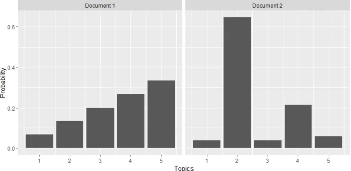
• Document-topic distribution: The uni-gram model only allows one topic for each docu-ment. If we relax the assumption and allow more than one topic within the same document (which is a natural relaxation), then each topic might contribute to some proportion of the documents. Of course, a single sentence, or maybe a single word, is possible to be contained within more than one topic. A latent assumption for topic models is thateach word is coming from only one topic. Hence, suppose we know exactly where each word is coming from, then the proportion of each topic’s contribution may be computed. Naturally, by definition, these proportions build a multinomial distribution. Figure 2.1 illustrates the distribution of two documents and five topics. Note that it is possible that the probability of some topics is zero for some specific documents. Hence, the total number of topics associated with the corpus might not be the same as the number of topics associated with each document. Similar to the topic-word distribution matrix, we use the document-topic distribution matrix to record these information. Suppose we have M documents within our corpus andKtopics associated with the corpus, the document-topic distribution matrix will be aK×M dimensional matrix such that each column indicates a document and each row indicates a topic. We usually use Θ to denote this matrix.

(29)

Figure 2.1: Example of Document-Topic distribution for 2 documents and 5 Topics Θ =         

Document1 Document2 Document3 ... DocumetM

topic1 θ11 θ12 θ13 . . . θ1M topic2 θ21 θ22 θ23 . . . θ2M .. . ... ... ... . .. ... topicK θK1 θK2 θK3 . . . θKM         

2.1.2

Bayes’ Theorem and Beyes’ Estimation

Bayes’ Theorem is one of the most important probability rules used in language models and topic models. Suppose we have two eventsAandB, then the event that bothAandB happens at the same time is denoted byA∩B. The probability associated with those events areP(A),P(B), andP(A∩B), respectively. We may use a Venn Diagram, Figure 2.2, to illustrate the situation:

The conditional probability is defined based on the the probability that both A and B

happened. The probability that event A occurs known event B already occurred is:

P(A|B) = P(A∩B)

(30)

Figure 2.2: A Venn Diagram illustrating the probability that both event happen. Areas represent probabilities

Similarly, the probability that even B occurs known that even A already occurred is:

P(B|A) = P(A∩B)

P(A) (2.2)

From equation 2.1 and 2.2, We have:

P(A∩B) =P(A|B)P(B)

P(A∩B) =P(B|A)P(A)

⇒P(A|B)P(B) =P(B|A)P(A)

⇒P(A|B) = P(B|A)P(A)

P(B)

The Bayes’ Theorem relates the probability before getting the evidence P(A) to the probability after getting the evidenceP(A|B). For this reason,P(A) is called the prior probability andP(A|B) is called the posterior probability. The fraction P_P(B₍_B|A₎) is called the likelihood ratio. Using these terms, Bayes’ theorem can be rephrased as ”the posterior probability equals the prior probability times the likelihood ratio”.

For topic modeling, Bayes’ Theorem is used as follows. Given two discrete random variables

X ==x1, x2, . . . , xn andY =y1, y2, . . . , ym, Bayes’ Theorem is:

P(X=xi|Y =yj) =

P(Y =yj|X =xi)P(X =xi)

P(Y =yj)

(31)

Based on the rule of total probability, P(Y = yj) = P n

i=1P(Y = yj, X = xi) = P n

i=1P(Y =

yj|X=xi)P(X =xi), equation 2.3 may be expressed as:

P(X =xi|Y =yj) =

P(Y =yj|X =xi)P(X =xi)

Pn

i=1P(Y =yj|X =xi)P(X =xi)

(2.4)

The idea of Bayesian generative process is constructed using Bayes’ Theorem as expressed in Equation 2.4. In general, one assumes no prior information about an article in the beginning. Hence, a distribution is selected as the standard distribution, and it is utilized to describe the topic model. The multinomial distribution is the natural selection to describe the topics and we will discuss it in the next section. After observing the article, one will update the standard distribution with the information gathered from the article.

The process of Bayesian estimation relies upon the structure of the article. Or more precisely, the way that we believe the article is constructed. Those beliefs are summarized into assumptions and different models are very likely to have different assumptions. Are the words independent to each other? Are there multiple topics within each article? How should one choose the standard dis-tribution (or prior)? How should one choose the likelihood function? Is there any other information, i.e. author name and affiliation, that might help in generating the posterior estimate?

One obvious conclusion is that there is no universal set of assumptions that fits for all documents. Some of those assumptions are able to be tested, but most of them can not. Moreover, similar with regression analysis, we need to understand that the model is almost always wrong (i.e. not completely consistent with the actual data generating process). But some of the models might produce a better estimate of the underlying truth than others. The only way to find it out is to evaluate the result, especially when the assumptions are unable to be checked.

2.1.2.1 Important Assumptions for Bayesian Estimation in Topic Model

There are still some baseline assumptions that everyone uses. One is that the conceptual population of all texts that might be constructed from the current language systems. One question we are interested in is that what is the basic building block of these texts? Linguists have dived deep into this topic. Chomsky [9] stated that the grammatical differences between human languages can be explained on the basis of a small number of hierarchically organized discrete principles and parameters. Mark C. Baker tried to construct principles and parameters theory in his book [1]. We

(32)

All Texts

Texts of Single Language

Texts of Single Document

Paragraph Sentence Phrase

Word Character

Figure 2.3: Layer of Texts

would like to point out that languages are discrete and texts are countable. This property allows us to select a proper discrete distribution while building our model. Figure 2.3 shows that all layers of texts are discrete. This is a prior belief in all topic models that we should know.

2.1.3

Multinomial Distribution and Dirichlet Distribution

The multinomial distribution is a natural choice in topic modeling. Suppose there is an random experiment that might generate a finite number of results, and the probability of those results that have been generated is a known fixed number. We may use a vector of zeros and ones to indicate which result is generated by the experiment. This vector is a random variable and we define the distribution of this random variable to be multinomial. If multiple independent experiments have been conducted, the multinomial random variable is defined with a vector that summarizes the number of each result that is generated.

Formally, suppose there are n trials of an experiment. For each trial, there is a set of k

possible out comes {x1, x2, . . . , xk} from the random experiment with a set of probability values

{p1, p2, . . . , pk} such that the P k

i=1pi = 1 and pi ≥0, the probability of xi happens is defined as

P(X =xi) =pi. Define~c= (c1, c2, . . . , ck) such that

(33)

then~cis said to have a multinomial distribution with parameters ~p= (p1, p2, . . . , pk) andn.

The probability mass function of a multinomial distribution is:

P(C= (c1, c2, . . . , ck)) = n! c1!. . . ck! pc1 1 . . . p ck k = (Pk i=1ci)! Qk i=1ci! k Y i=1 pci i

In the above equation, the fraction (

Pk i=1ci)!

Qk i=1ci!

is called the multinomial coefficient which quantifies the number of ways that we could divide the set of observationsninto subsets of size from

c1 tock. We may also use the Gamma function to represent this coefficient:

(Pk i=1ci)! Qk i=1ci! =Γ( Pk i=1ci+ 1) Qk i=1Γ(ci+ 1)

The topic-word distribution matrixϕand the document-topic distribution Θ contains the parameter of probabilities~pfor each multinomial distribution. Each element in vector~ptakes value from zero to one and is restricted by Pk

i=1pi = 1. In a uni-gram model, maximum likelihood

estimates of these probabilities are found using a frequentist approach. The Bayesian estimation method would assume that these probabilities follow some continuous distribution and try to update this prior belief using the observed data. The Dirichlet distribution and the multinomial distribution are two of the most commonly used prior distributions in the Bayesian approach.

The Dirichlet distribution, often denoted byDir(α), is a family of continuous multivariate probability distributions that take on positive real number values based on parameterα. The support of the Dirichlet distribution is the vector~x= (x1, x2, . . . , xk) where xi ∈(0,1) andP

k

i=1xi = 1. α

is often referred as the concentration parameter because it determines the spread of the realization from the distribution. Figure 1.3 in chapter 1 illustrated the effect ofα. Note that the support of the Dirichlet distribution is exactly the restriction of the parameters of the multinomial distribution. Hence, the α is also called the hyperparameter since it could be the parameter of the probability distribution of the probability parameter of multinomial distribution.

The probability density function of thekdimensional Dirichlet distribution is:

f(~p= (p1, . . . , pk)|~α= (α1, . . . , αk)) = Γ(Pk i=1αi) Qk i=1Γ(αi) k Y i=1 pαi−1 i

(34)

the vector α~ as a product of a scalar and a k-dimensional vector so that all entries are 1s: α~ =

α~1. Sometimes the~1 is ignored and the parameter of a Dirichlet distribution is simply stated as

α, which indicates a symmetric distribution. α is also known as the concentration parameter of the Dirichlet distribution. In general, one may use a base vector ~u such that α~ = α~u. If ~u is not a vector of ones, then the Dirichlet distribution is called asymmetric. Figure 1.3 shows five multinomial distributions drawn from five different Dirichlet distributions with different symmetric hyperparameters α ∈ [0.01,100]. As the parameter value increases, the random variable is more evenly spread over the possible outcomes and eventually almost uniformly distributed when the parameter value is very high.

As we mentioned in Chapter 1, the values of the hyperparameters are typically set using certain heuristics which are based on the document collection. Griffiths et al in [12] stated that for Latent Dirichlet allocation,α= 50

T whereT is the number of topics, andβ= 0.01 for the

document-topic and the document-topic-word distributions often generate reasonable results. Hence, these values are been considered the default for fitting Latent Dirichlet Allocation. The other way to estimate the concentration parameter is discussed in Minka [22], which generated maximum likelihood estimates of the parameters.

Asymmetric Dirichlet distributions also discussed by Wallach et al. [28]. She states that the asymmetric Dirichlet priors for document-topic distributions offer modeling advantages over symmetric priors in terms of evaluation based on perplexity. To find the best asymmetric base measures vector estimate, she applied a hierarchical structure of Dirichlet priors in which another symmetric Dirichlet distribution is considered as the prior of the base measures vector.

Based on equation 2.3, if we take X as the vector of probabilities from the underlying multinomial distribution, that follows a Dirichlet distribution before we observed the data set, and

Y is the observation of the multinomial distribution, then the posterior distribution P(X|Y) after we observe the data Y is also a Dirichlet distribution. In general, if the posterior distribution is from the same family of distributions as the prior these distributions are called a conjugate pair. Across different generative models it is more convenient to use conjugate pairs as they simplify the description of the generative process and provide mathematical convenience when deriving the posterior estimates.

There are many well known conjugate pairs such as Poisson, Beta-Binomial, Gamma-Exponential, Normal-Normal, etc. The initial distribution is the prior and the latter one is the

(35)

likelihood distribution. We have discussed the conjugate relationship above using the Dirichlet-Multinomial conjugate pair which is also used in the Latent Dirichlet Allocation. Next, we use a simple example to show how the concept of conjugate paires is utilized for topic modeling.

Suppose we have a topict= (p1, p2, . . . , p5) that is built upon a vocabulary which has five different tokens V ocabulary = {w1, w2, w3, w4, w5} and a document D1 that contains 100 words which is built solely upon this topic. Hence,D1 = (w1,1, w1,2, . . . , w1,100) and each w1,j is selected

from the vocabulary based on probabilities withint. By definition, the number of times each token is observed~c = (c1, c2, . . . , c5) should follows a multinomial distribution with parameter~p=t and

n= 100. Hence, we have:

~c∼M ultinomial(t,100) (2.5)

Furthermore, we assume thattis a random variable that follows a symmetric Dirichlet distribution with parameterα.

t∼Dir(α) (2.6)

This is called the prior distribution andαis the hyperparameter that can be interpreted as our prior belief before observing data. We would like to estimate the true distribution of~cwhich is equivalent with estimating the parameter t. Since t is a random variable, we would like to find its posterior distributionf(t|~c). Based on Bayes’ rule:

f(t|~c) = f(~c|t)f(t) f(~c) (2.7) Where f(~c|t) = (p1, p2, . . . , p5)) = Γ(P5 i=1ci+ 1) Q5 i=1Γ(ci+ 1) 5 Y i=1 pci i f(t|α) = Γ( P5 i=1α) Q5 i=1Γ(α) 5 Y i=1 pα_i−1

and f(~c) is the true probability that~c is observed, which is a constant fixed number. α is also a constant. There fore we can express f(t|~c) proportional to the following functions. and may be

(36)

ignored while computing the kernel of the distribution. Hence, we find the posterior distribution: f(t|~c)∝Γ( P5 i=1ci+ 1) Q5 i=1Γ(ci+ 1) Γ(P5 i=1α) Q5 i=1Γ(α) 5 Y i=1 pci i 5 Y i=1 pα_i−1 ∝ 5 Y i=1 pci i 5 Y i=1 pα_i−1 ∝ 5 Y i=1 pci+α−1 i (2.8)

Since they do not contribute to the kernel of the distribution, they should be able to re-generate through normalization.

The kernel of the Dirichlet distribution may be found by dropping all constant terms. Sup-poseθ∼Dir(αk), then

f(θ) =(α1, . . . , αk)) = Γ(Pk i=1αi) Qk i=1Γ(αi) k Y i=1 pαi−1 i ∝ k Y i=1 θαi−1 i (2.9)

Compare equations 2.8 and 2.9, we note the similarity of the kernel. More specifically, θ and t

are random variables, and αi and ci +α are the parameters. This demonstrates that the kernel

generated from equation 2.8 is from an asymmetric Dirichlet distribution with parameter ~c0 = (c1 +α, c2 +α, . . . , c5+alpha). Both the prior distribution and the posterior distribution are Dirichlet and we shown a proof of conjugacy for our example.

The conjugacy of Dirichlet-Multinomial also presents another interpretation of the hyper-parameterα. Note that ifci is the count of tokenwi contained in documentD1, thenαwill be the

prior belief of the number of times tokenwi shows up in documentD1. When αis small, then the

posterior distribution is more dependent on the observed document. Whenαis large relative to the document length, then the posterior is more dependent onα.

(37)

2.2

Topic Models

2.2.1

Unigram Model

The Unigram model is one of the earliest model developed for topic modeling. There are three assumptions for the unigram model:

• Each word/token is independent of other words.

• Each document only contains one topic

• Topics are not related between different documents.

Those assumptions are not been able to meet with real data. Consider a document that only contains a single sentence:

I have a ______ and I always love to play with him.

Semantically, a word like “boy”, “kid”, “dog”, “cat”, or “pet” make a lot more sense than “house”, “car” in the blank. And there exist words like “girl” or “mom” that don’t make sense at all because the word “him” points to male. This simple sentence shows that words are not independent of each other within a semantically consistent document. Random generation can be used to create research documents that satisfy this assumption, but that will be discussed later.

The second assumption could be true under a certain scenario. Suppose a writing test is given which asks participants to write about a specific topic. This should generate articles with a single topic. The problem here is that one can never verify if one article truly contains only a single topic. For example, suppose that we have two documents which are written by the participants of the writing test. Conceptually, these two documents should be both talking about the same topic. But these two documents should not be, and never will be, exactly the same. Even for a same large idea, people will write about it differently.

Mathematically, let V = (w1, w2, . . . , wn) be the vocabulary. D1 = (w1,1, w1,2, . . . , w1,n1)

be the document that containsn1 tokens. Then for the Unigram model we have:

(38)

where P(w1,i) =pi is the true probability of the underline topic generate this token w1,i. Hence,

the likelihood function of the documentD1 is:

L= n Y i=1 pci i (2.11)

whereci is the number of times tokenwi is presented in Di.

The log-likelihood function is:

logL= n X i=1 logpci i = n X i=1 cilogpi

with the restrictionPn

i=1pi= 1. Hence, we may compute the maximum likelihood estimation of~p:

ˆ ~ p= argmaxp~(logL+λ(1−P n i=1pi)) (2.12) ∂ ∂pi (logL+λ(1− n X i=1 pi)) = _∂p∂_ilogL+_∂p∂_i(λ(1−P n i=1pi)) = 0 (2.13) ∂ ∂pi Pn i=1cilogpi−λ_∂p∂ i Pn i=1pi = 0 (2.14) pi = xi λ (2.15)

Using the propertyPn

i=1pi= 1, we find thatλ=n. Hence,

ˆ ~ pM LE = ( c1 n, c2 n, . . . , cn n) (2.16)

In other words, the maximum likelihood estimation of the parameter for the topic is the vector of frequency of each word/token in the document.

Other than the unrealistic assumptions, there are still many problems with the Unigram model. For example, the maximum likelihood estimation only takes tokens that showed up in the document. This means that the token that didn’t show in the document will be assigned a probability zero. A smoothing algorithm might be used to solve this problem [6]. Bigram, Trigram, and N-gram models are built based on the Unigram model which relax the independent token assumption. These models do not use the Bayesian generative process and are considered as the traditional methods.

(39)

2.2.2

Latent Dirichlet Allocation

We briefly introduced the LDA model in Chapter 1. Latent Dirichlet Allocation (LDA), was originally introduced by Blei et al.[4] and it is one of the most important probabilistic topic model. It allows each single document to have multiple topics, thus introduces a document-topic distribution Θ, similarly with the topic-word distribution Φ. Imagine that each topic is a unique-colored urn of water, then to write an article we would like to select some of the urns and mix the water from different urns. In this way, if we have a total of K topics, Θ will be a K dimensional multinomial distribution. Under this set up, while writing articles, it is natural to firstly pick up a topic using Θ, then pick up a word from the selected topic usingΦ.

The key idea of LDA is thatΦand Θ are conditionally independent to each other if we know which word and topic the token has. Figure 2.4 shows the unrolled graph model of LDA. The top part of the graph (above themsign) is equivalent with the bottom part. Each circled node represents a random variable. The shaded nodes are observed variables and others are latent variables. Arrows represent the dependency between the random variables. The letter N, M, and T located in the bottom part of the graph (below the m sign) represent the number of repeated arrows in the top part of the graph.

2.2.2.1 Assumptions of LDA

• Documents contain multiple topics.

• The total number of topics of the corpus is a fixed number.

• Each document is assumed to be generated by a known process (to be describe next).

• Words are generated independently of other words (often called the bag-of-words assumption).

2.2.2.2 Generative process for LDA:

1. ChooseK, the number of topics in the collection; Chooseαandβ, the hyperparameter.

2. Draw ϕk ∼ Dir(β), k = 1, ..., K, V dimensional multinomial topic-word distribution for K

topics.

(40)

α θ z w ϕ β T N M β ϕ2 m ϕ1 . . . ϕT w1,1 w1,2 . . . w1,N w2,1 w2,2 . . . w2,N . . . wM,1 wM,2 . . . wM,N Z1,1 Z1,2 . . . Z1,N Z2,1 Z2,2 . . . Z2,N ZM,1 ZM,2 ZM,N . . . . . . θ1 θ2 . . . θM α

(41)

(a) Drawθd∼Dir(α) which is the parameter for the multinomial document-topic

distribu-tion. Thus θd determines how topics are mixed within any specific document.

(b) Then for each wordwi in document d:

i. Draw a topic indexzi∼M ultinomial(θd).

ii. Draw a wordwi ∼M ultinomial(ϕzi), which is the topic generated in the beginning

of the process.

2.2.2.3 Estimation in LDA:

There are three common method to do parameter estimation in LDA: Variational EM, expectation propagation, and Gibbs Sampling. The most widely used approach among those three is the Gibbs Sampling approach, followed by the Variational EM algorithm. In this section we discuss both approaches and go through the Gibbs Sampling method in detail since we choose to use Gibbs Sampling for the simulation discussed later. Heinrich[15] provides more details.

2.2.2.3.1 Gibbs Sampling

Gibbs Sampling is a variant of the Metropolis-Hasting method which constructs a Markov chain whose states are parameter settings and whose stationary distribution is the true posterior over those parameters. There are the original Gibbs Sampling method and the collapsed Gibbs method. We will go through details of the original Gibbs method.

Using the notation from the generative process, suppose we know~z, ~w, letzdbe the vector of

topic assignment for words in documentd1, then from equation 2.9, we know that the posterior of the

d-th documents’ document-topic distribution is also a multinomial distribution that has parameter

θd:

1_z

d,imight be considered as a multinomial distributed random variable that has parametern= 1, or a categorical

(42)

p(θd|zd, α) = p(zd|α, θd) p(zd|α) p(θd|α) (2.17) ∝ Nd Y n=1 M ulti(zd,n|θd)Dir(θd|α) (2.18) ∝ Nd Y n=1 (θd,k) I(zd,n=k)_Dir₍_θ d|α) (2.19) ∝ K Y k=1 θn (k) d d,k Dir(θd|α) (2.20) ∝Dir(θd|n~d+α), ~nd={n (k) d } K k=1 (2.21)

Wheren(_dk)refers to the number of times that topickhas been observed with a word from document

d. Similarly, p(ϕk|~z, ~w, β) = p(w~|~z, ϕk, β) p(w~|~z, β) p(ϕk|~z, β) (2.22) ∝ Y i:zi=k M ulti(wi|ϕk)Dir(ϕk|β) (2.23) ∝ V Y i=1 ϕn (i) k k,i Dir(ϕk|β) (2.24) ∝Dir(ϕk|n~k+α), ~nk={n (i) k } V i=1 (2.25)

Wheren(_ki) refers to the number of times that the word indexed byiin the vocabulary is initiated under topick.

Since for the Dirichlet distributionDir(p) we haveE[Xi] = Ppi_p

i, we will get the estimator:

d ϕk,t= n(_kt)+βt PV t=1(n (t) k +βt) (2.26) d θd,k = n(_dk)+αk PK k=1(n (k) d +αk) (2.27)

(43)

Using the bag-of-word assumption,wi is independent withw~¬iand also withz~¬i. Then the

denominator turns out to bep(z~¬i, ~w¬i|α, β). Thus, if we can find the joint distribution of~z andw~

givenαandβ, the Gibbs sampler will be completed. Note that the joint distribution can be factored:

p(w, ~~ z|α, β) =p(w~|~z, α, β)p(~z|α, β)

based on LDA’s assumption,w⊥α|~zand also~z⊥β. Thus,

p(w, ~~ z|α, β) =p(w~|~z, β)p(~z|α)

The first term can be find through an integral2_:

p(w~|~z, β) = Z p(w~|~z, Φ)p(Φ|β)dΦ = Z N Y i=1 p(wi|zi)p(Φ|β)dΦ = Z K Y k=1 V Y t=1 p(wi=t|zi=k)p(Φ|β)dΦ = Z K Y k=1 V Y t=1 ϕn (t) k k,t p(Φ|β)dΦ = Z K Y k=1 V Y t=1 ϕn (t) k k,t K Y k=1 1 ∆(β) V Y t=1 ϕβt−1 k,t dΦ = Z K Y k=1 1 ∆(β) V Y t=1 ϕn (t)+βt−1 k k,t dΦ = K Y k=1 ∆(n~k+β) ∆(β) , ~nk ={n (t) k } V t=1

2_{Here we use the notation that ∆(}_p_{) =}

Qdim(p)

k=1 Γ(pk)

Γ(Pdim(p)

k=1 pk)

(44)

Similarly, for the