One-Class Classifiers Based on
Entropic Spanning Graphs
Lorenzo Livi, Member, IEEE, and Cesare Alippi, Fellow, IEEE
Abstract— One-class classifiers offer valuable tools to assess the
presence of outliers in data. In this paper, we propose a design methodology for one-class classifiers based on entropic spanning graphs. Our approach also takes into account the possibility to process nonnumeric data by means of an embedding procedure. The spanning graph is learned on the embedded input data, and the outcoming partition of vertices defines the classifier. The final partition is derived by exploiting a criterion based on mutual information minimization. Here, we compute the mutual information by using a convenient formulation provided in terms of theα-Jensen difference. Once training is completed, in order to associate a confidence level with the classifier decision, a graph-based fuzzy model is constructed. The fuzzification process is based only on topological information of the vertices of the entropic spanning graph. As such, the proposed one-class classi-fier is suitable also for data characterized by complex geometric structures. We provide experiments on well-known benchmarks containing both feature vectors and labeled graphs. In addition, we apply the method to the protein solubility recognition problem by considering several representations for the input samples. Experimental results demonstrate the effectiveness and versatility of the proposed method with respect to other state-of-the-art approaches.
Index Terms—α-divergence, α-Jensen difference, entropic spanning graph, one-class classification, protein solubility.
I. INTRODUCTION
T
HE analysis of large volumes of data is hampered by many technical problems, including the ones related to the quality and interpretation of associated information. One-class classifier design is an important research endeavor [1], [2] that can be used to tackle the problems of anomaly/novelty detection or, more generally, to recognize outliers in incoming data [3]–[8]. Several different methods have been proposed in the literature, including clustering-based techniques, kernel methods, and statistical approaches (see [9] for a recent survey). A widespread approach considers data generating processes, whose “nominal conditions” are known by field experts, while nonnominal conditions are unknown; the fault recognition problem provides a pertinent example in this direction [10]. In such cases, a one-class classifier can be effectively trained to recognize the nominalManuscript received April 8, 2016; revised August 12, 2016; accepted September 12, 2016.
The authors are with the Department of Electronics, Information, and Bioengineering, Politecnico di Milano, 20133 Milan, Italy, and also with the Faculty of Informatics, Università della Svizzera Italiana, 6904 Lugano, Switzerland (e-mail: [email protected]; [email protected]).
Color versions of one or more of the figures in this paper are available online at http://ieeexplore.ieee.org.
Digital Object Identifier 10.1109/TNNLS.2016.2608983
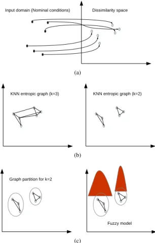
Fig. 1. Schematics illustrating the proposed classifier. The first step consists in mapping the input data to a dissimilarity space. A graph-based representation of the embedded data is then computed by minimizing the mutual information. Finally, in order to provide a confidence level associated with the classifier decision, the embedded data are fuzzified by exploiting only topological information derived from the graph-based representation. (a) Embedding. (b) kNN graph construction in dissimilarity space. (c) Graph partition and related fuzzification (colors online).
conditions only and reject, along with a confidence level, instances lying outside the nominal class.
In this paper, we present a novel methodology for con-structing one-class classifiers based on entropic spanning graphs [11] that extends a preliminary version appeared in [12]. The high-level steps behind the proposed classifier are given in Fig. 1. The first step consists in embedding the training set, representative of the nominal condition class, in a Euclidean space. The embedding is implemented by means of the dissimilarity space representation [13] that depends on a parametric dissimilarity measure defined in the input domain. An important consequence of this choice is that,
2162-237X © 2016 IEEE. Personal use is permitted, but republication/redistribution requires IEEE permission. See http://www.ieee.org/publications_standards/publications/rights/index.html for more information.
in principle, we are able to process any input data type (e.g., graphs, sequences, and other forms of nonnumerical data). Once the embedding vectors are generated, we construct a geometric (Euclidean) graph, whose vertices represent the embedded samples and the edges represent their Euclidean distances in the embedding space. Here, we use a k-nearest neighbor (kNN) graph, where k is considered to be a structural parameter. The model of the classifier is defined as one of the possible partitions of such vertices. In particular, we derive the partition by following a criterion based on mutual infor-mation minimization. The resulting connected components (clusters of vertices) form the decision regions (model) of the classifier.
As said earlier, the first step of the procedure consists in learning a dissimilarity representation of the input data. Dissimilarity (and kernel function) learning is a well-known research field in pattern recognition [14]. In general, research efforts in the field of dissimilarity learning focus on adapting well-known methods in the case of nonmetric distances; as an alternative, embeddings are developed [15], [16] bringing back the problem to the Euclidean geometric setting.
Dissimilarity representations might yield high-dimensional embedding vectors. Graph-based models of data are popular in pattern recognition, as in fact a graph allows to deal with the high dimensionality of the data by relying on topological infor-mation only [17], [18]. Among the many approaches, those based on kNN graphs are particularly interesting and more related to our work. For instance, Tomasev et al. [19], [20]ˇ exploit the concept of “hubness” of samples mapped to a kNN graph for designing clustering and classification sys-tems for high-dimensional data.
The methodology proposed here possesses several con-nections with other methods based on the concepts bor-rowed from information theory [21]. In fact, information-theoretic-based techniques are widely used in feature selection and image processing problems [22]–[29], as well as for devising clustering algorithms in both vector [30]–[34] and graph [35]–[38] domains. Finally, we comment that our con-tribution has some affinity with the information bottleneck method [39], [40]. In fact, such a method prescribes that the mutual information between the input and the compressed representation should be minimized, while at the same time enforcing the maximization of the mutual information of the compressed representation with the target/output signal. Here, we exploit only the unsupervised part of this approach by com-puting a compressed, cluster-, and graph-based representation of the input.
The novelty of our contribution can be summarized as follows.
1) A methodology for designing one-class classifiers, where the model of the classifier is obtained by exploit-ing a criterion based on mutual information minimiza-tion. To this end, we use a convenient formulation for the mutual information derived from the α-Jensen difference [41]. Such a measure can be directly com-puted by means of a kNN-basedα-order Rényi entropy estimator [42]. The final classifier, optimal according to the proposed criterion, is the one associated with the
partition among all possible partitions characterized by minimum statistical dependence between the clusters. 2) A fuzzy model built on top of the obtained graph
partition that provides a way to assign a confidence level, expressed in terms of membership degree to the nominal conditions class, to each test sample. The fuzzification mechanism is based only on topological properties of the vertices of the entropic spanning graph. Therefore, in principle, the method is capable to model clusters with arbitrary shapes.
We show the experimental results on both synthetic and real-world data sets for one-class classification, containing samples represented as feature vectors and labeled graphs. In this paper, in addition to evaluating the method on well-known benchmarks, we also face the challenging problem of protein solubility recognition [3]. Classification of proteins with respect to their solubility degree is a hard yet very important scientific problem, with consequences related to the folding of such macromolecules [43]. Here, we tackle the problem by representing a data set of proteins in several different ways: as sequences of symbols (amino acid identi-fiers), as labeled graphs (hence taking into account the folded structure), as sequences of numeric vectors encoding features of such graphs, and as feature vectors extracted from the graph structures (considering also postprocessed versions of such features). The possibility to deal with a given classification problem from several different angles (i.e., by using different data representations) without the need to fine tune the method is a valuable design asset of the proposed one-class classifier. The method presented here differs from our previous con-tribution [11] in a number of ways. First of all, here, we use a kNN graph for representing the samples in the embedding space, whereas in [11], we used a minimum spanning tree. In addition, the objective function for learning the model is based on mutual information, while in [11], we adopted a com-bination of entropy and modularity (to be maximized). Finally, the fuzzification of the graph-based model is implemented here by using only topological information of the entropic spanning graph vertices. In [11], instead, we used a more conventional centroid-based representation for the decision regions.
The remainder of this paper is structured as follows. In Section II, we provide the technical details related to the graph-basedα-order Rényi entropy estimator and related
α-Jensen difference. The reader might skip this section if already familiar with the basics. Section III provides the details on the proposed one-class classifier. In Section IV, we discuss the experimental results. Notably, in Section IV-A, we present the results on well-known benchmarking data sets (UCI and IAM). In Section IV-B, we discuss the results obtained on the problem of classifying proteins with respect to their solubility degree. Finally, in Section V, we draw our conclusions and offer future research directions.
II. RÉNYIENTROPYGRAPH-BASEDESTIMATION
A. Graph-Based Estimation of Rényi Entropy
Let X be a continuous random variable with probability density function (pdf) f(·). The Rényi entropy of orderα is
defined as Hα(X)= 1 1−αlog f(x)αd x , α≥0, α=1. (1) Whenα→1, (1) corresponds to the Shannon entropy.
Let us consider a data set S ⊂ Rm composed of n independent identically distributed m-dimensional realiza-tions xi ∈ S,i = 1,2, . . . ,n, with m ≥ 2. Let G be a
Euclidean graph, whose vertices denote the samples of S. An edge ei jconnecting xi and xj is weighted using the
Euclid-ean distance,|ei j| =d2(xi,xj). Theα-order Rényi entropy (1)
can be estimated according to a geometric interpretation of an entropic spanning graph of G [44]. Examples of spanning graphs used in the literature include the minimum spanning tree, kNN graph, Steiner tree, and TSP graph [45]–[52]. As we will discuss more formally in Section III, entropic spanning graphs are the key elements of our contribution, which will also be used to define the model of the classifier. Let Lγ(G) = e
i j∈G|ei j|
γ be the length of the entropic
spanning graph defined as the sum of all weights, where
γ ∈ (0,m) is a user-defined parameter defining the order of the Rényi entropy, α = (m −γ )/m. The γ parameter allows to focus on specific weights. For instance, withγ 1, it is possible to get rid of small weights in the summation; conversely, small values ofγmagnify the contribution of small weights. Although there is no optimal setting for all problems,
γ is typically set in order to obtainα=0.5. The Rényi entropy of order α∈(0,1)defined in (1) can be estimated as
ˆ Hα(G)=m γ log Lγ(G) nα −log(β(Lγ(G),m)) (2) where β(Lγ(G),m) is a constant term (i.e., it does not depend on the pdf) that is defined as β(Lγ(G),m)
γ /2 log(m/2πe). The entropy estimator (2) is a suitable choice for estimating information-theoretic quantities when process-ing high-dimensional data [42].
B. Rényi α-Divergence,α-Mutual Information, andα-Jensen Difference
Starting from the α-order Rényi entropy (1), it is possible to define other information-theoretic quantities, such as diver-gence and mutual information. Let f(·)and q(·)be two pdfs supported on the same domain. The Rényi α-divergence is defined as
Dα(f q)= 1
α−1log
f(x)αq(x)1−αd x (3) with α ∈ (0,1). Equation (3) operates as a measure of (nonmetric) dissimilarity between two distributions. In fact, it is nonnegative and is zero if and only if f(·)=q(·).
The mutual information between two distributions can be used to assess their statistical dependence. Said in other terms, mutual information can be seen as a measure of similarity between random variables, where the similarity is measured in terms of their dependence. In fact, we remind that two distributions are statistically independent if and only if their mutual information is zero. Let us consider our data set S. Calculating the α-divergence between the joint and product
of marginal distributions of S features allows to define the so-calledα-mutual information [41]. Such a measure computes the degree of statistical dependence between the components forming S (or, more generally, between d different random variables defined on the same domain). This is obtained by assessing f(·) and q(·) in (3) as the joint distribution and product of the marginals of S, respectively. Hence, mutual information and divergence provide powerful and complimen-tary tools to define dissimilarity-based recognition systems (in our case, one-class classifiers).
The α-Jensen difference, with α ∈ (0,1), is a useful measure of dissimilarity between two distributions that is defined as
Hα(β, f,q)
= Hα(βf +(1−β)q)− [βHα(f)+(1−β)Hα(q)] (4) whereβ∈ [0,1]allows for a linear convex combination of the pdfs. Since theα-order Rényi entropy (1) is strictly concave in f(·)forα∈(0,1)[41], the well-known Jensen’s inequality assures that (4) is nonnegative and degenerates to zero if and only if f(·)=q(·). This fact suggests to consider theα-Jensen difference (4) as a reliable alternative for theα-divergence (3) and hence also as a measure of statistical dependence between distributions. In particular, (4) is defined by considering only (combinations of)α-order Rényi entropy. Therefore, the
α-Jensen difference can be estimated directly by using bypass estimators for each entropy term appearing in (4), such as the graph-based entropy estimator shown in (2). Moreover, by Jensen inequality, it can be easily extended in order to handle d different pdfs as follows: Hˆα(β,G,d)= ˆHα(G)− d i=1 βiHˆα(Gi) (5) where βi = |Gi|/|G| and |Gi| indicates the number of
vertices in Gi, guaranteeing thus d
i=1βi = 1. In (5),
Gi,i =1, . . . ,d, are the d subgraphs of G representing the
d different pdfs under considerations.
Here, we use (5) as a measure of (statistical) dissimilarity between the d subgraphs Gi extracted from G derived during
the synthesis phase (see Section III).
III. ONE-CLASSCLASSIFIERBASED ONMUTUAL
INFORMATIONMINIMIZATION
This section describes our contribution. First, in Section III-A, we provide a high-level description of the main steps characterizing the proposed method. In Sections III-B and III-C, we describe, respectively, the synthesis of the model, the graph-based fuzzification, and how to use the classifier in the operational test modality. Finally, in Section III-D, we analyze the asymptotic computational complexity.
A. High-Level Description of the Proposed Method
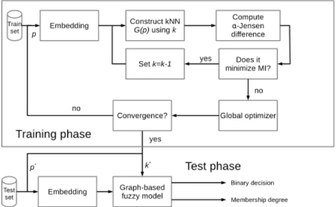
Fig. 2 provides a block scheme describing the main steps of the proposed one-class classifier. The classifier is applicable to any input domainX; as such, it operates also in domains
Fig. 2. Block scheme describing training and testing phases of the proposed one-class classifier.
of nongeometric data (e.g., nonnumeric data such as labeled graphs). Such a goal is achieved by first embedding the input data set S ⊂ X,|S| = n, into a m-dimensional Euclidean space. The embedding step can be described by a map φ : P(X)×P(X)× → Rn×m, where P(X) is the power
set of X and is a domain of numeric parameters of the input dissimilarity measure. A set of prototypes, R ⊆ S,
|R| = m ≤ n, called representation set, is used to compute the dissimilarity matrix, Dn×m, given as Di j = dI(xi,rj),
xi ∈ S and rj ∈ R, where dI : X ×X → R+ is a
nonnegative (bounded) dissimilarity measure. In order to give more flexibility to the method, we assume that dI(·,·)depends
on some (numerical) parameters, say p ∈ which, in turn, influence the resulting vector configuration in the embedding space. Developing the dissimilarity space representation (DSR) of S is a straightforward yet principled way to construct a Euclidean embedding space. Each input sample xi ∈ S is
represented by the corresponding row-vector xi of matrix D.
Therefore, the embedding step for the entire S is formally described as D=φ(S,R,p). This stresses that the embedding is controlled/influenced by both R and p. An important property of the DSR is that, if dI(·,·)is metric, distances in
the dissimilarity space are preserved up to a scaling factor equal to √m, that is, d2(xi,xj) ≤ dI(xi,xj)√m (Lipschitz
mapping). On the other hand, if dI(·,·) is not metric (for
instance, it violates the triangular inequality), it is possible to prove that such a property can be still satisfied by considering a constant related to the maximum violation of the triangular inequality [53].
Embedded data are then represented by means of a geomet-ric graph, G=(V,E). In this paper, we rely on kNN graphs. In kNN graphs, vertices V denote embedded samples in S, while edges their relations in terms of distance; each edge ei j ∈ E is assigned a weight wi j = d2(xi,xj). The
dimen-sionality of a DSR depends on the number of prototypes used during the computation of the dissimilarity matrix (the number of prototypes is the number of dimensions). Deter-mination of such prototypes is an important yet complex task; it is equivalent to a problem of feature selection. Sev-eral methods have been proposed in the literature (see [13] and references therein) to address this problem. However, all such methods are nontrivial in terms of computations, especially when contextualized within a more complex system.
Therefore, our choice was to avoid such computations and consider simple initializations of the prototypes—see the fol-lowing. Nonetheless, constructing G on the DSR also allows us to overcome/mitigate the problem of prototype selection, as in fact graphs are suitable for representing (possibly) high-dimensional data. In the following, we denote by G(p) the Euclidean graph constructed over the DSR of S computed using p for dI(·,·).
We define the model of the classifier in terms of decision regions by using the structural information derived from the kNN graph G(p). In particular, each connected component of G(p) forms a decision region. We propose a synthesis procedure for learning such decision regions based on the optimization of the α-Jensen difference (5). In doing so, we find a partition of the graph whose components denote high divergence, i.e., high statistical dissimilarity.
In order to provide a confidence level associated with the classifier decision, once training is complete, we fuzzify the obtained graph-based representation G(p). In practice, a mem-bership degree is assigned to each vertex of the kNN graph. Such membership degrees are based only on the topological information provided by G(p), hence allowing to model data with complex geometric structures.
A test sample is classified during the operational modality by first mapping it into the DSR. Then, the sample is fuzzified by using the related topological information. The classifier provides two types of decisions regarding the membership of test samples to the nominal conditions class: a binary and a membership degree.
B. Training by Minimizing the Mutual Information
We propose a learning approach for synthesizing the clas-sifier model by exploiting theα-Jensen difference (5) using a kNN graph. Let us define the objective function
η(p,k)= 1
1+Hˆα(β,G(p),d(k)) ∈ [0,1] (6) which basically converts the α-Jensen difference (5) in a similarity measure. Although, formally speaking, (6) cannot be thought as a form ofα-mutual information, we argue that it could be used as a proxy for its computation. In fact, (6) assumes one when the divergence is zero (i.e., when all dis-tributions are equal) and tends to zero as the divergence grows (see [41] for further examples). The optimization problem describing the one-class classifier model synthesis is, hence, formulated as
min
k,p η(p,k) (7)
where k ≥ 1 is the parameter of the kNN spanning graph that acts here a structural parameter, defining the upper bound for the partition order d. In fact, the number d=d(k)≥1 of connected components (subgraphs) of the resulting kNN graph depends on k, as made explicit in (6). Parameters p affect the dissimilarity measure used to construct the DSR. For instance, when the input domain X corresponds to Rn, then dI(·,·)
could be defined as a Euclidean metric with p as a vector of weights (or as a covariance matrix). Therefore, the choice
Algorithm 1 Training of the One-Class Classifier
Input: A dataset S of n samples
Output: P(G(p∗))
1: Determine the prototypesR⊆S
2: while Global optimization cycle do
3: Get an instance of the parameters, p
4: Construct the DSR ofS using Rand p
5: for k=√n, ...,1 do
6: Construct the kNN spanning graph using k
7: Derive the partition, P(G(p))k, by grouping vertices
according to the resulting connected components
8: Compute the α-divergence (5) 9: Evaluate objective (6)
10: if η(p,k) > η(p,k+1)then
11: Exit for loop at line 5
12: end if
13: end for
14: if Global convergence then
15: Store best k∗=k and p∗= p
16: return P(G(p∗))with d =d(k∗)components
17: end if
18: end while
of p influences also the topology of the kNN graph. With (7) we propose to minimize the dependence (or equivalently, maximize the independence) between the distribution of the resulting connected components, i.e., the clusters of con-nected vertices derived from the kNN graph. The optimization problem (7) consists in searching for the model order d through k and the parameters p of the dissimilarity measure that maximize the estimatedα-Jensen difference (5) calculated on the resulting graph partition. Please notice that valid solu-tions for (7) also include kNN graphs with only one connected component (i.e., fully connected graphs).
Algorithm 1 delivers the pseudocode describing the pro-posed model synthesis strategy. A partition P(G(p))is formed by means of the connected components of the kNN graph. A global loop at line 2 searches for the parameters p (that can be a vector) of the input dissimilarity measure affecting the DSR of S and hence the resulting kNN graph. In this paper, all input samples are used as prototypes for the DSR, i.e., R=S. The high dimensionality of the resulting DSR does not pose a serious problem, since all operations are based on the kNN graph. However, when the cardinality of S is large, we subsample the data set with a randomized selection scheme. At line 5, we perform an additional loop where we decrease the structural parameter k, hence forming a nondecreasing number d ≤ k of connected components (subgraphs) in the related kNN graph. Within this loop, we use (5) to estimate the
α-Jensen difference in the dissimilarity space. The entropy of the entire data set, Hˆα(G), is estimated using k+1 for the kNN graph. This is performed to allow for a different number of edges in the resulting kNN graph with respect to the total number of edges in the subgraphs derived by using k.
The algorithm proceeds iteratively by increasing the structural complexity of the model, i.e., by decreasing k. We use a heuristic at line 10 to terminate the search: when
(6) starts to increase, then the model complexity should not be increased further. This choice is justified by considering the nature of our problem (7) which, in fact, consists solely in minimizing the statistical dependence. A global conver-gence criterion (line 14) is used to stop the search on the parameters p. Since our objective is to be able to process any type of input data, here, we use a derivative-free approach for searching for the best-performing p. However, different search methods (e.g., gradient-based approaches) could be used by considering specific problem instances, such as when processing feature vectors. The global convergence criterion is activated when a maximum number of iterations is performed or the objective function falls below a thresholdτ 0. C. Fuzzy Model Based on Vertex Centrality
We exploit the graph-based representation G(p∗), where p∗ denotes the optimal dissimilarity measure parameters, for constructing a fuzzy model. A fuzzy set is assigned to each of the d subgraphs, by defining the fuzzification mechanism based only on the topological importance (centrality) of ver-tices. In particular, we use the vertex closeness centrality as a measure of importance of the vertices.
Let Gi be the i th subgraph of G (note that we omit
parameters p∗ only for the sake of simplicity). The closeness centrality of a vertexv is computed as
χi(v)= u=v
2−dGi(v,u) (8)
where dGi(v,u)is the weighted topological distance between
vertices v and u in Gi. We remind that Gi is a geometric
graph constructed over a dissimilarity space. Therefore, each edge has a weight that is given by the Euclidean distance among the corresponding samples in the dissimilarity space.
Letχi∗=maxvχi(v)be the maximum closeness centrality
value for the i th subgraph. We define χˆi(v) and χˆi,
respec-tively, as the vertex-specific difference and the lth percentile of all differences with respect to the maximum closeness centrality value, that is
ˆ
χi(v)=χi∗−χi(v) (9) ˆ
χi =percentilev(χˆi(v),l). (10)
Note that l in (10) can be adjusted depending on the problem at hand; for instance, l = 50 gives the median value. The membership degree of v to the i th subgraph is defined as
μi(v)=exp −χˆi(v)2 2χˆi2 . (11)
It is important to note that, as a consequence of the definition of (8)–(11), there might be more than one vertex in a sub-graph with membership equal to 1 (i.e., with equal closeness centrality).
When a new test sample x has to be evaluated, we assign to it the maximum among the membership values computed for each of the d subgraphs
μ(x)= max
Equation (12) is used to define the membership of test samples to the class of nominal data: 0 implies that a sample does not belong to that class, 1 indicates that it completely belongs to it, while everything in-between provides a mem-bership degree to the class of nominal data.
The binary decision rule, instead, operates by checking if
ˆ
χj(x)≤ ˆχj (13)
where j =arg maxi=1,2,...,dμi(x).
In order to implement (12), we need to: 1) embed x in the dissimilarity space induced by using p∗ and 2) add a vertex corresponding to x , say vx, iteratively to each
subgraph Gi,i = 1,2, . . . ,d, with k∗ new edges, where
p∗ and k∗ are derived during training. It is worth noting an important fact here. When vx is added to Gi, the resulting
kNN graph might change globally: several nearest neighbor relations might be affected. Therefore, oncevx is added to Gi,
we recompute the kNN graph and perform the operations described by (8)–(13).
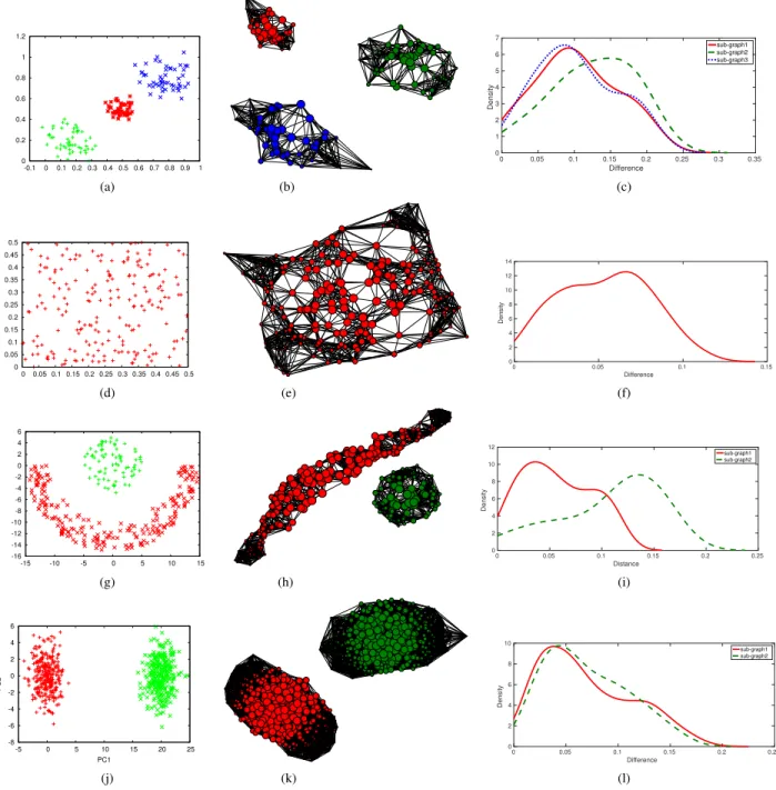
Fig. 3 shows the four sample data sets that are useful to highlight key modeling features of the proposed method. For each data set (left panels), we show the resulting graph-based model (middle panels) learned during the synthesis; the fuzzification is performed by using the same training data. We also show the density (right panels) of the differences with respect to the vertex with maximum closeness centrality (considering all derived subgraphs). Such information is useful to understand how the threshold (13) is derived. The first data set in Fig. 3(a) shows a simple case with spherical and separated clusters. The resulting graph model [Fig. 3(b)] is composed by three decision regions. The size of each of vertex reflects the membership degree assigned to the corresponding sample by using the herein described graph-based fuzzification mechanism; the edge lengths are monotonically related to the corresponding Euclidean distances. It is easy to recognize the correspondence with the geometry of the data set. In the second example [Fig. 3(d)], we show a uniformly distributed data set. The proposed method learns a graph-based model [Fig. 3(e)] with only one decision region, as in fact the data possess no structure. However, samples still present differences in terms of centrality/membership degree. In order to stress the capability of the proposed method to model data with intricate geometry, we show in Fig. 3(g) a data set with two clusters having very different geometric properties. The resulting graph-based model shown in Fig. 3(h) correctly finds two decision regions having good resemblance with the geometry of the data set. Finally, in Fig. 3(j), we show the first two principal components of a 100-D, normally distributed data set with two well-defined clusters. The graph-model in Fig. 3(k) shows that it is possible to perfectly reconstruct such two clusters, even by considering the high dimensionality of the data.
In all cases, corresponding densities shown on the right-hand side panels [see Fig. 3(c), (f), (i), and (l)] denote the nontrivial distributions of closeness centrality differences (9). This highlights the need to consider suitable percentiles (10) of such distributions in order to compute the binary decisions of the classifier (13).
D. Analysis of Computational Complexity
We assume to perform the global optimization in Algorithm 1 with a genetic algorithm. The computational complexity of the training phase is O(IPF), where I is the maximum number of iterations, P is the population size, and F is the cost of the fitness function. In the following, we include all relevant terms and factors in the analysis of the computational complexity, even those that do not influence the asymptotic behavior. The cost of F can be expressed as the sum of the following terms:
O(F1)=O(nr D) O(F2)=O( √ n F3) O(F3)=O r n2 kNN + n components + nk α−Jensen . (14) O(F1) accounts for the construction of the DSR with
n samples and r prototypes, where D is the computational complexity associated with the dissimilarity measure for the input data, which, depending on the specific case, might not be negligible. O(F2) accounts for the loop at line 5,
which repeats at most √n times the operations described by F3. O(F3)describes the cost associated with kNN graph
construction, determination of the connected components, and computation ofα-Jensen difference (5). The asymptotic com-putational complexity for training is, hence, upper bounded by O(n5/2).
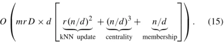
Let us now focus on the computational complexity of the test phase (normal operating mode; Section III-C). At this stage, the data are partitioned into d ≥ 1 components (the decision regions). Each test sample is sequentially assigned to each of those components. The related kNN subgraphs are updated with corresponding calculation of closeness centrality and determination of membership degree of the test sample. The computational complexity is given by
O ⎛ ⎜ ⎝mr D×d ⎡ ⎢ ⎣r (n/d)2 kNN update +( n/d)3 centrality + n/d membership ⎤ ⎥ ⎦ ⎞ ⎟ ⎠. (15) In (15), m is the number of test samples. The first cost, mr D, is due to the embedding of the test data in the dissimilarity space. There are three main costs involved in the computational complexity for testing the model: update of the kNN subgraph related to a decision region, calcula-tion of closeness centrality for the vertices in the subgraph, and computation of membership degree of the test sample [see (8)–(13)]. The asymptotic computational complexity of the test stage depends thus on the order of d. If d =1 and assuming m n, then the worst case is O(n3), which is
given by the cost of well-known Floyd–Warshall algorithm for computing all-pair shortest paths in a weighted undirected graphs.
Asymptotic computational complexity for constructing a kNN graph can be lowered by considering more advanced, yet approximate solutions [17], [22]. Similarly, the vertex centrality can be computed with approximated versions of closeness centrality [54] or by using other measures of central-ity (importance) of vertices taken from the complex network
Fig. 3. Functioning of the graph-based fuzzification on four simple data sets. The graphs are the result of the model training with Algorithm 1. Fuzzification is performed on the training set. Size of vertices in the middle panel is proportional to the related membership degree in decision regions. Position of graph vertices in the middle panel plots is not related to the position of the related samples in the input domain. On the right-hand side panels, we show the density of the differences, for each identified subgraph, with respect to the vertex having maximum closeness centrality [see (9)]. (a) Sample data set. (b) Graph-based model. (c) Density of differences for each subgraph. (d) Uniform data set. (e) Graph-based model. (f) Density of differences. (g) Crescent-full moon data set. (h) Graph-based model. (i) Density of differences for each subgraph. (j) First two principal components of a 100-D data set. (k) Graph-based model. (l) Density of differences for each subgraph (colors online).
literature. In addition, it is worth noting that, when processing input samples represented as numeric vectors, there is no need to perform the embedding step devised in our method. This would result in a significant reduction of the computational complexity costs (in terms of both time and space) discussed here.
IV. EXPERIMENTALRESULTS
Experimental evaluation is first performed (Section IV-A) on UCI and IAM benchmarking data sets. The proposed one-class classifier is denoted as EOCC-MI throughout the experiments.
In addition, in Section IV-B, we address the important problem of protein solubility recognition. In this case, we take into account and compare several data representation for proteins, including sequences, graphs, and feature vectors.
EOCC-MI depends on two hyperparameters: the threshold
τ ≥ 0 for terminating the search in Algorithm 1 and l expressing the lth percentile of the distribution of closeness centrality differences (see Section III-C). These two hyperpa-rameters allow to fine-tune the classifier with respect to the problem at hand. However, we noted that, in general, setting
TABLE I
UCI DATASETSCONSIDERED INTHISPAPER
TABLE II
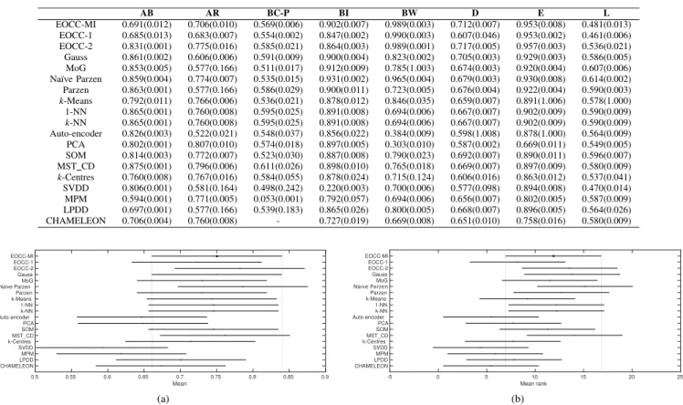
AUC TESTSETRESULTS ONUCI DATASETS
Fig. 4. Global ranking of AUC results in Table II. The proposed classifier, EOCC-MI, denotes competitive performances with respect to the state-of-the-art classifiers taken into account. Missing value for CAMELEON on BC-P is replaced with the mean value over the data set. (a) Ranking with two-way ANOVA. (b) Ranking with Friedman test.
considered problems. Therefore, in the following, we adopt such settings.
A. UCI and IAM Data Sets
The UCI data sets taken into account are shown in Table I. Data sets and results for comparison are taken from [55]; data sets are not preprocessed in any way. AUC results and related standard deviation are shown in Table II. EOCC-MI performs well on all UCI data set with two exceptions: AB and L data sets. In fact, for these two data sets, EOCC-MI results are significantly lower than the average outcome ( p <0.0001). Global ranking is shown in Fig. 4. EOCC-MI denotes global statistics that are not significantly different from the other classifiers taken into account. Considering the two-way ANOVA test [Fig. 4(a)], EOCC-MI is globally ranked at the fourth position. When taking into account the Friedman test, instead, it is ranked eighth [Fig. 4(b)].
TABLE III
IAM DATASETSTAKENINTOACCOUNT
Table III shows some information related to the IAM data sets [56]. The samples (from digital images to proteins) are represented as labeled graphs, with attributes on both vertices and edges. AUC values are reported in Table IV. Results are compared with the previous experiments [11]. EOCC-MI denotes the comparable results with the other two classifiers. However, we note statistically significant differences in two cases (G and P data sets), where EOCC-2 achieves better results. It is worth underlying that, in EOCC-2 [11], the final
TABLE IV
AVERAGEAUC (WITHRELATEDSTANDARDDEVIATION)ANDAVERAGESERIALCPU TIME(TRAINING/TESTEXPRESSED INSECONDS)
FORIAM DATASETS INTABLEIII. RESULTS FOREOCC-1ANDEOCC-2 ARETAKENFROM[11]. RESULTS INBOLDDENOTESTATISTICALLYSIGNIFICANTDIFFERENCES
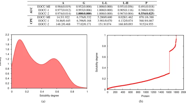
Fig. 5. Density and normalized solubility degree of the E. coli proteins. (a) Density of the 3173 E. coli proteins with respect to the normalized solubility degree. (b) Normalized solubility degree of the 1811 proteins taken into account. The two classes are clearly recognizable.
model is derived by means of cross validation. As such, it is expected to be more accurate in terms of recognition capability. However, as shown in the second block of Table IV, EOCC-2 is significantly slower (from tens to hundreds of times slower) in terms of computing CPU time required for training [software is written in C++ and implemented on an Intel(R) Core(TM) i7-4710HQ CPU 2.50 GHz]. This fact suggests that EOCC-MI offers a good compromise between computational cost and recognition performance.
B. Protein Solubility Recognition
Protein folding refers to the chemicophysical process trans-forming the primary structure of a protein into a 3-D, active molecular conformation [43]. Despite the recent progresses in protein structure characterization and prediction, protein folding is still a largely unsolved problem in biophysics and related computational sciences [57]. This fact is due to a multitude of causes, such as the large number of residues involved in the process (protein molecules contain from tens to thousands of residues) and the different energy constraints defining the (thermodynamic) energy landscape. The process of folding strictly competes with the aggregation process, that is, with the tendency of proteins to also establish inter-molecular bonds. Aggregation propensity is intimately related to the degree of solubility of a molecule [58]. This results in the formation of large multimolecular aggregates which, analogously to what happens with artificial polymers, are insoluble and hence precipitate in solution [59]. Aggregation propensity of proteins, in turn, is strongly related to problems occurring during the folding process, resulting in pathologies
(misfolding diseases), such as Alzheimer and Parkinson [43]. Therefore, studying the solubility degree of proteins is of utmost importance in protein science.
Niwa et al. [60] analyzed in a strictly controlled setting the aggregation/solubility propensity of a large set (3173) of E. coli proteins. Proteins having difficulty in perform-ing the foldperform-ing autonomously (i.e., without the help of the so-called chaperones) tend to aggregate and hence precipi-tate in the solution (water in the experiment). The 3173 E. coli proteins denote a bimodal distribution of (normalized) solubility, with many proteins having a low solubility degree and only very few soluble proteins [see Fig. 5(a)]. In order to conceive a classification problem, a suitable threshold for the solubility must be identified within the solubility range. We consider the[0,0.3]and[0.7,1]intervals for determining insoluble and soluble proteins. The resulting data set contains 1811 proteins, whose solubility range shown in Fig. 5(b) clearly denotes the presence of two different classes: proteins with low and high solubility degrees, respectively. However, although the intervals have the same length and are positioned at the extremes of the solubility range, the resulting data set is very imbalanced, containing 1631 insoluble and only 180 soluble proteins.
We denote the data set containing 1811 proteins as DS-1811-SEQ. Samples in this data set are represented as variable-length sequences of amino acid identifiers (21 different characters that identify the amino acids). The dissimilarity measure for the input, dI(·,·), is implemented
by using the well-known Levenshtein sequence alignment algorithm. Folded proteins find a better representation in terms
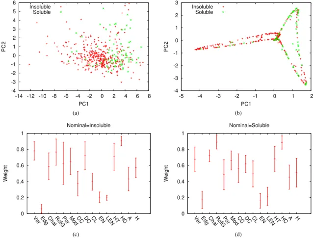
Fig. 6. First two components of DS-454-PCA and DS-454-KPCA. The difficulty of the problem can be appreciated from the high overlap between the two classes. Average weight values learned by the algorithm on DS-454-FEATURE, considering insoluble and soluble proteins for the nominal class. (a) PCA. (b) Kernel PCA. (c) Average weights for features with insoluble as nominals. (d) Average weights for features with soluble as nominals.
of networks. Therefore, we also consider the corresponding graph-based representation of such proteins. Vertices of such graphs are labeled with 3-D numeric vectors, which convey a compressed version of the information provided by the chemicophysical attributes of the related amino acids. Edges are labeled with the Euclidean distance between the residues. However, among the 1811 proteins, only 454 currently have a resolved 3-D structure in the Protein Data Bank.1 As a consequence, we were able to generate a data set of labeled graphs containing 454 proteins. This data set is denoted as DS-454-GRAPH. In this case, dI(·,·)is implemented by using
a graph edit distance algorithm [61].
By starting from DS-454-GRAPH, we develop four additional data representations. The first one contains the sequences of 3-D numeric vectors associated with the graph vertices. This data representation is obtained by “seriating” the graphs. Therefore, a sequence contains a number of elements equal to the number of vertices in the related graph (see [62] for details on the seriation algorithm). In this case, dI(·,·) is implemented by using the dynamic time
warping algorithm, equipped with a weighted Euclidean distance for computing the distances between the 3-D vectors composing the sequences. In addition, we also extracted a collection of numeric features from the graph representations,
1http://www.rcsb.org/pdb/home/home.do
by considering topological characteristics describing both structural and dynamical features of such graphs. This consists in mapping each graph in DS-454-GRAPH with a 15-D feature vector. We denote this data set as DS-454-FEATURE. Finally, in order to reduce dimensionality of DS-454-FEATURE, we postprocess such data with principal component analysis and the related kernel version. In the first case, we retain the first five components (explaining≈85% of total variance); in the second case, instead, we retain only three components. The two resulting data sets are denoted as DS-454-PCA and DS-454-KPCA, respectively. First two components of DS-454-PCA and DS-454-KPCA are shown in Fig. 6(a) and (b), respectively. In the last three cases, we always use the weighted Euclidean metric for dI(·,·).
Table V shows the AUC results obtained by considering all data representations. We take into account both the cases for defining the class of nominal data, i.e., either the soluble and insoluble proteins. Results obtained on DS-1811-SEQ are not comparable with the others, due to the different numbers of samples. However, related AUC values show that, in both cases, the results are comparable with the others. Let us focus on the remaining five data representations. When the nominal class is populated with insoluble proteins, significantly better results ( p<0.0001) are obtained on DS-454-GRAPH. On the other hand, when considering the soluble proteins as nominal, better results ( p < 0.0001) are obtained on DS-454-SEQV.
TABLE V
AUC TESTSETRESULTS ONALLDATAREPRESENTATIONSTAKENINTO
ACCOUNT FOR THEPROBLEM OFPROTEINSOLUBILITYRECOGNITION
This suggests that the rich information provided by the graph representations of proteins is useful for discriminating the degree of protein solubility.
It is worth stressing that the results with DS-454-FEATURE are significantly better than those obtained with both DS-454-PCA and DS-454-KPCA. In fact, AUC is significantly higher ( p < 0.0001 with respect to DS-454-PCA; with DS-454-KPCA, p < 0.0003 when insoluble proteins are considered as nominal and p < 0.0001 otherwise). This fact suggests that the selection of the weights p∗ based on the proposed mutual information minimization criterion also results in an effective mechanism of feature selection. In Fig. 6(c) and (d), we show the average values of the weights found by the algorithm for the two scenarios for the nominal class. Significant features with high average weight are preserved in both cases, yet with some small numerical differences. The most relevant features are the number of vertices (“Ver”), number of chains in the molecule (“Chai”), radius of gyration (“RofG”), modularity of the graph (“Mod”), average degree (“DC”), and two diffusion characteristics called heat trace (“HT”), and heat content (“HC”), calculated by using Laplacian matrix of the graphs.
V. CONCLUSION
In this paper, we presented a design methodology for one classifiers based on entropic spanning graphs. Input data are first mapped into a dissimilarity representation, allowing to deal with several input data representations. Embedding vectors are constructed by using a (parametric) dissimilarity measure. An entropic spanning graph is then constructed over the embedded data and successively processed to derive a model for the classifier. Entropic spanning graphs are well known in the literature for providing a nonparametric approach to estimate information-theoretic quantities, such as entropy and divergence. Here, we have also proposed to use a kNN graph (a particular instance of entropic spanning graphs) to define the model of the one-class classifier. In particular, decision regions have been derived by partitioning the kNN graph vertices considering the related connected components induced during training. We proposed to guide the selection of the best-performing graph partition by using an optimization criterion based on mutual information minimization. Notably, we searched for the best-performing parameters p of the input dissimilarity measure and k, inducing a partition of order d with minimum statistical dependence. This was performed to ensure the maximum independence between the different clusters of vertices (i.e., the decision regions forming the model). Mutual information has been computed by exploiting
a convenient formulation defined in terms of the α-Jensen difference.
In order to associate a confidence level with each classifier decision, after training, we constructed a fuzzy model on the resulting graph partition. A membership degree is assigned to each vertex of the kNN graph, denoting the membership of the related input sample to the class of nominal data. The fuzzification of the vertices is based only on the topological information derived from the kNN graph, hence allowing to model data sets with complex geometries.
Experimental evaluation of the proposed one classifier is performed on both benchmarking data sets (containing sam-ples represented as either feature vectors and labeled graphs) and by facing an application involving protein molecules. Benchmarking results on numerical data showed that the proposed method performs well with respect to several state-of-the-art one-class classifiers. A drawback of our approach is the computational complexity, which does not scale well when the sample size grows [it is of the order of O(n5/2)]. On the other hand, our approach allows to deal with a wide range of problems, regardless of the data representation adopted for the input data.
Here, we tackled the important problem of recognizing the degree of solubility of the data sets of E. coli pro-teins. Such data have been analyzed by considering several different data representations, including sequences, labeled graphs, and numeric features. The possibility to address a given problem from different angles is a valuable design asset characterizing the proposed method. The analysis of protein solubility revealed the possibility to achieve good performances by considering different data representations, especially with those based on labeled graphs. In addition, in the case of numeric features used to represent proteins, the proposed method provided a selection of the most relevant ones that could be exploited for further analyses.
Future research efforts will focus on improving the compu-tational complexity, by conceiving approximate or alternative algorithmic solutions for the computation of kNN graph and vertex centrality. In addition, it could be interesting to conceive a variant of the method able to dealing with time-variant environments. In fact, it is reasonable to think that the nominal conditions might change over time, for instance due to concept drifts (e.g., aging) affecting the data generating process. The one-class classifier should be able to adapt the model on-the-fly with such new nominal conditions, possibly forming new decision regions and/or integrating the already existing ones with new data.
REFERENCES
[1] F. Dufrenois, “A one-class kernel Fisher criterion for outlier detection,” IEEE Trans. Neural Netw. Learn. Syst., vol. 26, no. 5, pp. 982–994, May 2015.
[2] F. Dufrenois and J. C. Noyer, “One class proximal support vector machines,” Pattern Recognit., vol. 52, pp. 96–112, Apr. 2016. [3] L. Livi, A. Giuliani, and A. Sadeghian, “Characterization of graphs
for protein structure modeling and recognition of solubility,” Current Bioinformatics, vol. 11, no. 1, pp. 106–114, Jan. 2016.
[4] J. Oster, J. Behar, O. Sayadi, S. Nemati, A. E. W. Johnson, and G. D. Clifford, “Semisupervised ECG Ventricular beat classification with novelty detection based on switching kalman filters,” IEEE Trans. Biomed. Eng., vol. 62, no. 9, pp. 2125–2134, Sep. 2015.
[5] C. Alippi, G. Boracchi, and M. Roveri, “Hierarchical change-detection tests,” IEEE Trans. Neural Netw. Learn. Syst., doi: 10.1109/TNNLS.2015.2512714, to be published.
[6] G. Boracchi and M. Roveri, “Exploiting self-similarity for change detection,” in Proc. Int. Joint Conf. Neural Netw. (IJCNN), Jul. 2014, pp. 3339–3346.
[7] M. Radovanovi´c, A. Nanopoulos, and M. Ivanovi´c, “Reverse nearest neighbors in unsupervised distance-based outlier detection,” IEEE Trans. Knowl. Data Eng., vol. 27, no. 5, pp. 1369–1382, May 2015. [8] Z. S. Abdallah, M. M. Gaber, B. Srinivasan, and S. Krishnaswamy, “Any
novel: Detection of novel concepts in evolving data streams,” Evolving Syst., vol. 7, no. 2, pp. 73–93, 2016.
[9] M. A. F. Pimentel, D. A. Clifton, L. Clifton, and L. Tarassenko, “A review of novelty detection,” Signal Process., vol. 99, pp. 215–249, Jun. 2014.
[10] E. De Santis, L. Livi, A. Sadeghian, and A. Rizzi, “Modeling and recognition of smart grid faults by a combined approach of dissimi-larity learning and one-class classification,” Neurocomputing, vol. 170, pp. 368–383, Dec. 2015.
[11] L. Livi, A. Sadeghian, and W. Pedrycz, “Entropic one-class classifiers,” IEEE Trans. Neural Netw. Learn. Syst., vol. 26, no. 12, pp. 3187–3200, Dec. 2015.
[12] L. Livi and C. Alippi, “One-class classification through mutual infor-mation minimization,” in Proc. IEEE Int. Joint Conf. Neural Netw., Vancouver, BC, Canada, Jul. 2016, pp. 1–8.
[13] L. Livi, A. Rizzi, and A. Sadeghian, “Optimized dissimilarity space embedding for labeled graphs,” Inf. Sci., vol. 266, pp. 47–64, May 2014. [14] F.-M. Schleif and P. Tino, “Indefinite proximity learning: A review,”
Neural Comput., vol. 27, no. 10, pp. 2039–2096, 2015.
[15] B. Xiao, E. R. Hancock, and R. C. Wilson, “Geometric characterization and clustering of graphs using heat kernel embeddings,” Image Vis. Comput., vol. 28, no. 6, pp. 1003–1021, 2010.
[16] R. C. Wilson, E. R. Hancock, E. Pekalska, and R. P. W. Duin, “Spherical and hyperbolic embeddings of data,” IEEE Trans. Pattern Anal. Mach. Intell., vol. 36, no. 11, pp. 2255–2269, Nov. 2014.
[17] J. Chen, H.-R. Fang, and Y. Saad, “Fast approximate k-nn graph construction for high dimensional data via recursive Lanczos bisection,” J. Mach. Learn. Res., vol. 10, pp. 1989–2012, Dec. 2009.
[18] J. R. Bertini, Jr., L. Zhao, R. Motta, and A. D. A. Lopes, “A nonpara-metric classification method based on K-associated graphs,” Inf. Sci., vol. 181, no. 24, pp. 5435–5456, 2011.
[19] N. Toma˘sev, M. Radovanovi´c, D. Mladeni´c, and M. Ivanovi´c, “The role of hubness in clustering high-dimensional data,” IEEE Trans. Knowl. Data Eng., vol. 26, no. 3, pp. 739–751, Mar. 2014.
[20] N. Toma˘sev, M. Radovanovi´c, D. Mladeni´c, and M. Ivanovi´c, “Hubness-based fuzzy measures for high-dimensional k-nearest neighbor classifi-cation,” Int. J. Mach. Learn., vol. 5, no. 3, pp. 445–458, 2014. [21] B. Chen, Y. Zhu, J. Hu, and J. C. Principe, System
Parame-ter Identification: Information CriParame-teria and Algorithms. AmsParame-terdam, The Netherlands: Elsevier, 2013.
[22] J. Kybic and I. Vnuˇcko, “Approximate all nearest neighbor search for high dimensional entropy estimation for image registration,” Signal Process., vol. 92, no. 5, pp. 1302–1316, 2012.
[23] J. R. Vergara and P. A. Estévez, “A review of feature selection methods based on mutual information,” Neural Comput. Appl., vol. 24, no. 1, pp. 175–186, 2014.
[24] H. Liu, J. Sun, L. Liu, and H. Zhang, “Feature selection with dynamic mutual information,” Pattern Recognit., vol. 42, no. 7, pp. 1330–1339, 2009.
[25] M. R. Sabuncu and P. Ramadge, “Using spanning graphs for effi-cient image registration,” IEEE Trans. Image Process., vol. 17, no. 5, pp. 788–797, May 2008.
[26] A. Bardera, M. Feixas, I. Boada, and M. Sbert, “Image registration by compression,” Inf.Sciences, vol. 180, no. 7, pp. 1121–1133, 2010. [27] G. Brown, A. Pocock, M.-J. Zhao, and M. Luján, “Conditional likelihood
maximisation: A unifying framework for information theoretic feature selection,” J. Mach. Learn. Res., vol. 13, no. 1, pp. 27–66, 2012. [28] J. H. Plasberg and W. B. Kleijn, “Feature selection under a complexity
constraint,” IEEE Trans. Multimedia, vol. 11, no. 3, pp. 565–571, Apr. 2009.
[29] K. S. Balagani and V. V. Phoha, “On the feature selection criterion based on an approximation of multidimensional mutual information,” IEEE Trans. Pattern Anal. Mach. Intell., vol. 32, no. 7, pp. 1342–1343, Jul. 2010.
[30] V. V. Vikjord and R. Jenssen, “Information theoretic clustering using a k-nearest neighbors approach,” Pattern Recognit., vol. 47, no. 9, pp. 3070–3081, 2014.
[31] A. Alush, A. Friedman, and J. Goldberger, “Pairwise clustering based on the mutual-information criterion,” Neurocomputing, vol. 182, pp. 284–293, Mar. 2015.
[32] A. Kraskov, H. Stogbauer, R. G. Andrzejak, and P. Grassberger, “Hier-archical clustering using mutual information,” Eur. Phys. Lett. (EPL), vol. 70, no. 2, p. 278, 2005.
[33] P. Shen and C. Li, “Distributed information theoretic clustering,” IEEE Trans. Signal Process., vol. 62, no. 13, pp. 3442–3453, Jul. 2014. [34] E. Gokcay and J. C. Principe, “Information theoretic clustering,” IEEE
Trans. Pattern Anal. Mach. Intell., vol. 24, no. 2, pp. 158–171, Feb. 2002. [35] M. Rosvall and C. T. Bergstrom, “An information-theoretic framework for resolving community structure in complex networks,” Proc. Nat. Acad. Sci. USA, vol. 104, no. 18, pp. 7327–7331, 2007.
[36] E. Ziv, M. Middendorf, and C. H. Wiggins, “Information-theoretic approach to network modularity,” Phys. Rev. E, vol. 71, p. 046117, Apr. 2005.
[37] A. Raj and C. H. Wiggins, “An information-theoretic derivation of min-cut-based clustering,” IEEE Trans. Pattern Anal. Mach. Intell., vol. 32, no. 6, pp. 988–995, Jun. 2010.
[38] M. Yu et al., “Hierarchical clustering in minimum spanning trees,” Chaos, Interdiscipl. J. Nonlinear Sci., vol. 25, no. 2, p. 023107, 2015. [39] S. Still, “Information bottleneck approach to predictive inference,”
Entropy, vol. 16, no. 2, pp. 968–989, 2014.
[40] N. Slonim, N. Friedman, and N. Tishby, “Multivariate information bottleneck,” Neural Comput., vol. 18, no. 8, pp. 1739–1789, 2006. [41] H. Neemuchwala, A. O. Hero, III, and P. Carson, “Image matching using
alpha-entropy measures and entropic graphs,” Signal Process., vol. 85, no. 2, pp. 277–296, 2005.
[42] A. O. Hero, III, B. Ma, O. J. J. Michel, and J. Gorman, “Applications of entropic spanning graphs,” IEEE Signal Process. Mag., vol. 19, no. 5, pp. 85–95, Sep. 2002.
[43] K. A. Dill and J. L. MacCallum, “The protein-folding problem, 50 years on,” Sci., vol. 338, no. 6110, pp. 1042–1046, 2012.
[44] A. O. Hero and O. J. J. Michel, “Asymptotic theory of greedy approx-imations to minimal k-point random graphs,” IEEE Trans. Inf. Theory, vol. 45, no. 6, pp. 1921–1938, Sep. 1999.
[45] N. Leonenko, L. Pronzato, and V. Savani, “A class of Rényi information estimators for multidimensional densities,” Ann. Statist., vol. 36, no. 5, pp. 2153–2182, 2008.
[46] B. Bonev, F. Escolano, D. Giorgi, and S. Biasotti, “Information-theoretic selection of high-dimensional spectral features for structural recogni-tion,” Comput. Vis. Image Understand., vol. 117, no. 3, pp. 214–228, 2013.
[47] D. Pál, B. Póczos, and C. Szepesvári, “Estimation of Rényi entropy and mutual information based on generalized nearest-neighbor graphs,” in Advances in Neural Information Processing Systems, J. D. Lafferty, C. K. I. Williams, J. Shawe-Taylor, R. S. Zemel, and A. Culotta, Eds. Red Hook, NY, USA: Curran Associates, Inc., 2010, vol. 23, pp. 1849–1857.
[48] D. Stowell and M. D. Plumbley, “Fast multidimensional entropy esti-mation by k-d partitioning,” IEEE Signal Process. Lett., vol. 16, no. 6, pp. 537–540, Jun. 2009.
[49] J. A. Costa and A. O. Hero, III, “Determining intrinsic dimension and entropy of high-dimensional shape spaces,” Statist. Anal. Shapes, H. Krim and A Jr.. Yezzi, Eds. Birkhäuser Boston, MA, USA, 2006. [50] J. A. Costa and A. O. Hero, “Manifold learning using Euclidean
k-nearest neighbor graphs,” in Proc. IEEE Int. Conf. Acoust., Speech, Signal Process., vol. 3. Montreal, QC, Canada, May 2004, pp. 988–991. [51] K. Sricharan and A. O. Hero, III, “Weighted k-NN graphs for Rényi entropy estimation in high dimensions,” in Proc. IEEE Statist. Signal Process. Workshop, Nice, France, Jun. 2011, pp. 773–776.
[52] J. A. Costa and A. O. Hero, III, “Geodesic entropic graphs for dimension and entropy estimation in manifold learning,” IEEE Trans. Signal Process., vol. 52, no. 8, pp. 2210–2221, Aug. 2004.
[53] E. P¸ekalska and R. P. W. Duin, The Dissimilarity Representation for Pattern Recognition: Foundations and Applications. Singapore, World Scientific, 2005.
[54] M. Borassi, P. Crescenzi, and A. Marino. (Jul. 2015). “Fast and sim-ple computation of top-k closeness centralities.” [Online]. Available: https://arxiv.org/abs/1507.01490
[55] Results on One-Class Classification, assessed on 2016. [Online]. Available: http://homepage.tudelft.nl/n9d04/occ/index.html
[56] K. Riesen and H. Bunke, “IAM graph database repository for graph based pattern recognition and machine learning,” in Structural, Syntactic, and Statistical Pattern Recognition, N. da Vitoria Lobo et al., Eds. Orlando, FL, USA: Springer, 2008.
[57] P. G. Wolynes, “Evolution, energy landscapes and the paradoxes of protein folding,” Biochimie, vol. 30, pp. 50–56, Dec. 2014.
[58] F. Agostini, M. Vendruscolo, and G. G. Tartaglia, “Sequence-based prediction of protein solubility,” J. Molecular Biol., vol. 421, nos. 2–3, pp. 237–241, 2012.
[59] A. Giuliani, R. Benigni, J. P. Zbilut, C. L. Webber, Jr., P. Sirabella, and A. Colosimo, “Nonlinear signal analysis methods in the elucidation of protein sequence-structure relationships,” Chem. Rev., vol. 102, no. 5, pp. 1471–1492, 2002.
[60] T. Niwa et al., “Bimodal protein solubility distribution revealed by an aggregation analysis of the entire ensemble of Escherichia coli proteins,” Proc. Nat. Acad. Sci., vol. 106, no. 11, pp. 4201–4206, 2009. [61] L. Livi and A. Rizzi, “The graph matching problem,” Pattern Anal.
Appl., vol. 16, no. 3, pp. 253–283, 2013.
[62] L. Livi, A. Giuliani, and A. Rizzi, “Toward a multilevel representation of protein molecules: Comparative approaches to the aggregation/folding propensity problem,” Inf. Sci., vol. 326, pp. 134–145, Jan. 2016.
Lorenzo Livi (M’14) received the B.Sc. and M.Sc. degrees from the Department of Computer Science and the Ph.D. degree from the Department of Infor-mation Engineering, Electronics, and Telecommuni-cations, Sapienza University of Rome, Rome, Italy, in 2007, 2010, and 2014, respectively.
He has been with the ICT industry. From 2014 to 2016, he was a Post-Doctoral Fellow with Ryerson University, Toronto, ON, Canada. In 2016, he was a Post-Doctoral Fellow with the Politecnico di Milano, Milan, Italy, and Università della Svizzera Italiana, Lugano, Switzerland. He is currently a Lecturer (Assistant Professor) in data analytics with the Department of Computer Science, University of Exeter, Exeter, U.K. His current research interests include computational intelligence methods, time series analysis, and complex dynamical systems, with focused applications in computational biochemistry and biophysics.
Dr. Livi is a member of the Editorial Board of Applied Soft Computing (Elsevier) and a Regular Reviewer for several international journals, including the IEEE TRANSACTIONS ONFUZZYSYSTEMSand Information Sciences (Elsevier).
Cesare Alippi (F’06) received the M.Sc. degree in electronic engineering in 1990, and the Ph.D. degree from the Politecnico di Milano, Milan, Italy, in 1995.
He has been a Visiting Researcher with University College London, London, U.K., the Massachusetts Institute of Technology, Cambridge, MA, USA, ESPCI ParisTech, Paris, France, CASIA (RC), and A*STAR (SIN). He is currently a Full Professor of Information Processing Systems with the Politecnico di Milano, and of Cyber-Physical and Embedded Systems with the Università della Svizzera Italiana, Lugano, Switzerland. He holds five patents, has published a monograph entitled Intelligence for Embedded Systems (Springer, 2014), and co-authored over 200 papers in international journals and conference proceedings. His current research interests include adaptation and learning in nonstationary environments and intelligence for embedded systems.
Dr. Alippi is a Distinguished Lecturer of the IEEE CIS, a member of the Board of Governors of INNS, the Vice-President education of the IEEE CIS, an Associate editor (AE) of the IEEE Computational Intelligence Magazine, the past AE of the IEEE TRANSACTIONS ON INSTRUMENTATION AND
MEASUREMENTSand the IEEE TRANSACTIONS ONNEURALNETWORKS, and a member and the Chair of other IEEE committees. In 2004, he received the IEEE Instrumentation and Measurement Society Young Engineer Award; in 2013, he received the IBM Faculty Award. He also received the 2016 IEEE TNNLS outstanding paper award and the 2016 INNS Gabor award. Among the others, he was the General Chair of the International Joint Conference on Neural Networks in 2012, the Program Chair in 2014, and the Co-Chair in 2011. He was the General Chair of the IEEE Symposium Series on Computational Intelligence 2014.