Approximate Nearest Subspace Search with Applications to Pattern Recognition
Ronen Basri
†Tal Hassner
†Lihi Zelnik-Manor
‡†
Weizmann Institute of Science
‡
California Institute of Technology
Rehovot, Israel
Pasadena, CA 91125, USA
{ronen.basri, tal.hassner}@weizmann.ac.il [email protected]
Abstract
Linear and affine subspaces are commonly used to de-scribe appearance of objects under different lighting, view-point, articulation, and identity. A natural problem arising from their use is – given a query image portion represented as a point in some high dimensional space – find a subspace near to the query. This paper presents an efficient solution to the approximate nearest subspace problem for both lin-ear and affine subspaces. Our method is based on a simple reduction to the problem of nearest point search, and can thus employ tree based search or locality sensitive hashing to find a near subspace. Further speedup may be achieved by using random projections to lower the dimensionality of the problem. We provide theoretical proofs of correctness and error bounds of our construction and demonstrate its capabilities on synthetic and real data. Our experiments demonstrate that an approximate nearest subspace can be located significantly faster than the exact nearest subspace, while at the same time it can find better matches compared to a similar search on points, in the presence of variations due to viewpoint, lighting etc.
1. Introduction
Linear and affine subspaces are a common means of rep-resenting information in computer vision and pattern recog-nition applications. In computer vision, for example, sub-spaces are often used to capture the appearance of objects under different lighting [4, 18], viewpoint [21, 19], artic-ulation [7, 20], and even identity [3, 5]. Typically, given a query image portion, represented as a point in high di-mensional space, a database of subspaces is searched for the subspace closest to the query. A natural problem which arises from this type of search problems is, can the near-est (or a near) subspace be found faster than a brute force sequential search through the entire database?
R.B and T.H. were supported in part by the A.M.N. Fund for the promotion of science, culture and arts in Israel and by the European Community grant IST-2002-506766 Aim@Shape. The vision group at the Weizmann Insti-tute is supported in part by the Moross Foundation. L.Z.-M. was supported by ONR grant N00014-06-1-0734 and NSF grant CMS-0428075. Author names are ordered alphabetically due to equal contribution.
The related problem of finding the nearest neighbor within a database of high dimensional points has become an important component in a wide range of machine vision and pattern recognition applications. As such, it has attracted considerable attention in recent years, and a number of ef-ficient algorithms forapproximate nearest neighbor(ANN) search have been proposed (e.g., [2, 8, 11, 13]). These algo-rithms achieve sub-linear search times when locating a near, not necessarily the nearest neighbor, suffices. In light of the success of ANN methods our goal is to design an approxi-mate nearest subspace(ANS) algorithm for efficient search through a database of subspaces.
We present an ANS algorithm, based on a reduction to the problem of point ANN search. Our algorithm can thus work in concert with any ANN method, enjoying fu-ture improvements to these algorithms. For a query point and a database of n subspaces of dimension kembedded in Rd, ANS query running time, using our construction, isO(kd2) +T
AN N(n, d2), where TAN N(n, d)is the run-ning time for a choice of an ANN algorithm, on a database of n points inRd. We achieve further speedup by using random projections to lower the dimensionality of the prob-lem. Our method is related to recent work by Magen [15], who reduced ANS to a nearest hyperplane search. Magen’s method, however, requiresO(nd2)preprocessing time and space while our preprocessing requires onlyO(nkd2).
We next describe our method, provide theoretical proofs of correctness and error bounds of our construction, and present both analytical and empirical analysis. We further demonstrate our method’s capabilities on synthetic and real data, with an emphasis on image and image-patch retrieval applications.
2. Nearest Subspace Search
Thenearest subspace problemis defined as follows. Let
{S1,S2, ...,Sn} be a collection of linear(or affine) sub-spaces inRd, each with intrinsic dimensionk. Then, given a query pointq∈ Rd, denote bydist(q,Si)the Euclidean distance between the queryqand a subspaceSi,1≤i≤n, we seek the subspace S∗ that is nearest to q, i.e., S∗ =
arg minidist(q,Si).
We approach the nearest subspace problem by reducing it to the well explored nearest neighbor (NN) problem for points. To that end we seek to define two transformations,
u=f(S)andv=g(q), which respectively map any given subspaceSand query pointqto pointsu,v∈ Rd0for some
d0, such that the distancekv−ukincreases monotonically withdist(q,S). In particular, we derive below such trans-formations for whichkv−uk2 = µdist2(q,S) +ν for
some constantsµandν. This is summarized below.
Linear Subspaces: We represent a linear subspaceS by a
d×k matrixS with orthonormal columns. Our transfor-mations mapS andqontoRd0 withd0 =d(d+ 1)/2. For
a symmetricd×dmatrixAwe define an operatorh(A), wherehrearranges the entries of A into a vector by tak-ing the entries of the upper triangular portion ofA, with the diagonal entries scaled by1/√2, i.e.,
h(A) = (a√11 2, a12, ..., a1d, a22 √ 2, a23, ..., add √ 2) T ∈ Rd0 (1) Finally, we denote byn= √2h(I) ∈ Rd0 (I denotes the identity matrix) a vector whose entries are one for each di-agonal entry inh(.)and zero elsewhere. We are now ready to define our mapping. Denote by
u = f(S) =−h(I−SST) +αn v = g(q) =γ h(qqT) +βn , (2) with α = d−k d√2 β = −kqk 2 d√2 γ = 1 kqk2 r k(d−k) d−1 . (3)
We show this construction satisfies the following claim.
Claim 2.1 kv−uk2 =µdist2(q,S) +ν
, where the con-stantsµ=γ >0andν≥0satisfies
ν = 1−k d k− r k(d−k) d−1 !
In particular,µ= 1/kqk2andν = 0whenk= 1for alld,
andµ≈√k/kqk2andν ≈k−√kwhenkd.
Affine Subspaces: We represent a k dimensional affine
subspaceAby a(d+ 1)×(d−k)matrixZˆwhose firstd
rows contain orthonormal columns, representing the space orthogonal toA, and last row contains a vector of offsets. We further represent the query by homogeneous coordi-nates, qˆ = (qT,1)T. Our transformations mapA andqˆ toRdˆ0, where nowdˆ0 = (d+ 1)(d+ 2)/2 + 1. Finally,
using the(d+ 1)×(d+ 1)matrixIA = diag{1, ...1,0}, we denote by nˆ = (√2h(IA),0) ∈ Rd 0 . We define our mapping as follows: ˆ u = fˆ(A) =−(h( ˆZZˆT),ˆc(A)) + ˆαnˆ ˆ v = gˆ(q) = ˆγ(h(ˆqˆqT),0) + ˆβnˆ. (4) with ˆ c(A) = s M4− kZˆZˆTk2 f ro 2 ˆ α = d−k d√2 ˆ β = −kqk 2 d√2 ˆ γ = 1 kqk2 r dM4−(d−k)2 d−1 , (5)
with a sufficiently large constantM (see Section 2.3). We show this construction satisfies the following claim:
Claim 2.2 kvˆ−uˆk2 = ˆµdist2(q,A) + ˆν
, with constants
ˆ
µ >0andˆν≥0.
The remainder of this section provides a detailed deriva-tion of these claims. We begin by focusing on the case of linear subspaces (Section 2.1) and investigate the properties of our derivation (Section 2.2). Later on (Section 2.3) we extend this derivation to the case of affine subspaces.
2.1. Linear subspaces
Our derivation is based on the relation between inner products and norms in Euclidean spaces. We first show that the squared distance between a pointqand a subspaceS,
dist2(q,S), can be written as an inner product, and then that the vectors obtained in this derivation have constant norms. This leads to a basic derivation, which we later mod-ify in Section 2.2 to achieve the final proof of Claim 2.1. Let
S be ad×kmatrix whose columns form an orthonormal basis forS, and letZbe ad×(d−k)matrix whose columns form an orthonormal basis to the null space ofS. The dis-tance betweenqandS is given bydist(q,S) =kZZTqk, where ZZTq is the projection ofq onto the columns of
Z. SinceZZT is symmetric andZTZ =I, implying that
(ZZT)T(ZZT) =ZZT, we obtain:
dist2(q,S) =qTZZTq. (6) This can be written as
qTZZTq= d X i=1 d X j=1 [ZZT ⊗qqT]ij, (7)
where we use the symbol ’⊗’ to denote the Hadamard (element-wise) product of two matrices. In other words, if
we rearrange the elements of the matricesZZT andqqT as two vectors inRd2then the squared distance can be written as an inner product between those vectors.
Exploiting the symmetry of bothZZT andqqT we can embed the two vectors inRd0 withd0 =d(d+ 1)/2. This
can be done using the operatorh(.)defined earlier in (1):
¯
u = −h(ZZT)∈ Rd0
¯
v = h(qqT)∈ Rd0. (8)
Note, thatZZT = I−SST, and so it is unnecessary to explicitly construct a basis for the null space. It can now be readily verified that
¯ uTv¯=−1 2 X ij [ZZT ⊗qqT] =−1 2dist 2 (q, S). (9) Therefore, ku¯−v¯k2=ku¯k2+k¯vk2+ dist2(q, S), (10) and it is left to show that bothku¯kandk¯vkare constants. Next we show that k¯uk is constant for all subspaces of a given intrinsic dimension k, while kv¯k varies with the query. To see this notice that
ku¯k2= (1/2)kZZTk2
F ro, (11)
where k.kF ro denotes the Frobeneous norm, defined as
kZZTk2
F ro = Tr(ZZT(ZZT)T), and Tr(.) denotes the trace of a matrix. Using the identityZZT(ZZT)T =ZZT and the properties of the trace we obtain Tr(ZZT) =
Tr(ZTZ) = Tr(I) =d−k, and soku¯k2= (1/2)(d−k),
implying that our transformation maps each subspace in the database to a point on the surface of a sphere. Similarly,
kv¯k2 = (1/2)kqqTk2
F ro = (1/2)kqk4 is a constant that depends onq.
In summary, we found a mapping u¯ = ¯f(S)andv¯ = ¯ g(q)which satisfies ku¯−v¯k2= dist2 (q,S) +1 2(d−k+kqk 4), (12)
where the additive constant depends on the query pointq
and is independent of the database subspaceS.
Subspaces of varying intrinsic dimension: When the
database {S1, , ...,Sn} contains subspaces with different intrinsic dimensionk1, ..., kn, we obtain a different norm for each: k¯uik2 = (1/2)(d−k
i). We can handle this by introducing an additional entry to eachu¯ias follows:
˘
ui = −(h(ZZT),c˘(Si))∈ Rd0+1 ˘
v = (h(qqT),0)∈ Rd0+1. (13)
withc˘(Si)) = p
(1/2)(ki−kmin), wherekminis the di-mension of the thinnest subspace in the database. Note, that the additional entry does not changek¯vkor the inner prod-uctu¯Tv¯.
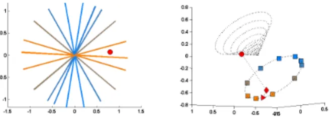
Figure 1.The geometry of our mapping.Example of 1D subspaces in R2, color coded according to distance from a query (left) and their
map-ping (right). In the basic construction (8) the database lines and potential queries are mapped respectively to a ring and a cone inR3. The figure
shows the query mapped to the cone, then projected to the hyperplane and scaled to lie on the ring.
2.2. The geometry of the mapped database
The transformations introduced earlier in Section 2.1 map all the linear subspaces of dimension kto points on the surface of a sphere of radiusp(d−k)/2inRd0. Fur-ther inspection of this mapping reveals that all these points also lie on an affine hyperplane. This is a consequence of Tr(ZZT) = d−k, which implies that the sum of the components ofu¯that correspond to the diagonal element of
ZZTis constant. At the same time query points are mapped to the surface of a spherical cone, whose apex is in the ori-gin and whose main axis is orthogonal to this hyperplane. We can use these facts to further project the query to the same hyperplane, and thus reduce the additive constant in-troduced to the distances by our mapping. This is illustrated in Figure 1, which shows an example of a database of 1D linear subspaces in 2D and their mapping to points in 3D. As is discussed later in Section 3 this will further improve the performance of the nearest neighbor search.
Using the vectorndefined in the beginning of Section 2 we can express the hyperplane by the following formula
−√2nTu¯=d−k. (14) We can shift this hyperplane so that it goes through the ori-gin by settingu= ¯u+αnwithα= (d−k)/(d√2). The hyperplane after this translation is then given bynTu= 0. Given a query qand its mapped version v¯ we seek to projectv¯ onto this translated hyperplane. That is, we seek a scalarβsuch thatv= ¯v+βnlies on the hyperplane:
nT(¯v+βn) = 0. (15) Notice that√2nTv¯=kqk2andnTn=d, and so
kqk2+√2dβ= 0,
(16) from which we obtainβ =−kqk2/(d√2). Therefore, we
can map the query pointqtov= ¯v+βnand by this reduce the additive constant in (12) by(kqk2+d−k)2/(2d).
By uniformly scaling the query point q we can bring it even closer to the mapped database. Note that uniform
scaling of q maintains the monotonicity of the mapping. Specifically, we can scaleqsuch that its norm after scal-ing becomes((d−k)k/(d−1))1/4. Then, after mapping
and projection the query will fall on the intersection of the database sphere and its hyperplane. The obtained squared distances after these transformations will be relatedlinearly to the original squared distances byµdist2(q,S) +ν with the constantsµandν as given in Claim 2.1. Interestingly, in the case of subspaces of rank 1ν = 0, and so ifqlies on
S thenuandvcoincide regardless ofd. For subspaces of higher rank (1< k < d)ν >0and souandvcannot coin-cide because the subspaces only sparsely occupy the sphere. Note, that the case of subspaces of varying dimension is somewhat more complicated since in this case the mapped subspaces lie on parallel hyperplanes according to their in-trinsic dimension. In this case the query can only be pro-jected to the nearest hyperplane.
2.3. Affine subspaces
With few modifications similar transformations can be derived for databases containing a collection of affine spaces. An affine subspace A is represented by a linear subspaceS, provided as ad×kmatrixSwith orthonormal columns (or by its null space, provided as ad×(d−k) ma-trixZ) and a vector of offset valuest∈ Rd−k. Below we denote byZˆthe(d+ 1)×(d−k)matrix whose firstdrows containZand last row containstT. Given a queryq∈ Rd we use homogenous coordinates, denotingˆq= (qT,1)T.
We define a mapping similar to that of linear spaces, this time usingZˆ andˆqinstead. The columns ofZˆare not or-thonormal due to the additional last row. To account for this we will need to slightly modify our mapping, as follows.
˜
u = fˆ(A) =−(h( ˆZZˆT),cˆ(A))∈ Rdˆ0
˜
v = ˆg(q) = (h(ˆqqˆT),0)∈ Rdˆ0. (17)
˜
u and v˜ lie in Rdˆ0, where now dˆ0 = (d + 1)(d +
2)/2 + 1. The last entry is added to make the norm of u˜ equal across the database. To achieve this we set
ˆ c(A) = q(M4− kZˆZˆTk2 f ro)/2, where kZˆZˆ Tk2 f ro = kZZTk2 f ro+2kZtk 2+ktk2=d−k+3ktk2andMis a
pos-itive constant;M must be sufficiently large to allow taking the square root for all the affine subspaces in the database (thus it is determined by the affine space with largestktk). Note, that we set the last entry of v˜ to zero, so that the last entry of u˜ does not affect the inner product of u˜Tv˜. Consequently,ku˜k2 = (1/2)M4,kv˜k2= (1/2)kˆqk4, and ˜ uTv˜ =−1 2 P ij[ ˆZZˆ T ⊗qˆqˆT] = −1 2dist 2 (q,A), and we obtain ku˜−v˜k2= dist2(q,A) +1 2(M 4+ kˆqk4), (18)
where the additional constant depends on the query pointq
and is independent of the database subspaceA.
Similar to the case of linear subspaces, the affine sub-spaces too are mapped to the intersection of a sphere (of ra-diusM2/√2) and a hyperplane−√2nTu˜ =d−k, and so the query can be projected into this hyperplane in the same way as in Section 2.2, yielding the result stated in Claim 2.2.
3. Nearest Neighbor Search
Once the subspaces in the database are mapped to points we can find the nearest subspace to a query by applying a nearest neighbor search for points. Naturally, we wish to employ an efficient solution to this problem. The prob-lem of nearest neighbor search has been investigated exten-sively in recent years, and algorithms for solving both the exact and approximate versions of the problem exist. For example, for a database containing npoints inRd, exact nearest neighbor can be found by transforming the prob-lem to a point location probprob-lem in an arrangement of hy-perplanes [1], which can in turn be solved using Meiser’s ray shooting algorithm in timeO(d5logn)[14]. This
algo-rithm, however, requires preprocessing time and storage of
O(nd+1), which may be prohibitive for typical vision
ap-plications.
Approximate solutions to the nearest neighbor problem can achieve comparable query times using a linear (O(dn)) preprocessing time and storage. These algorithms return, given a query and a specified constant > 0, a point whose distance from the query is at most a (1 +)-factor larger from the distance of the nearest point from the query. Tree based techniques [2] perform this task using at most
O(dd+1−dlogn), and despite the exponential term they appear to run much faster than a sequential scan even in fairly high dimensions. Another popular algorithm is the locality sensitive hashing (LSH) [8, 11]. LSH is designed to solve thenear neighborproblem, in which givenrandwe seek a neighbor of distance at mostr(1 +)from the query, provided the nearest neighbor lies within distance r from the query. LSH finds a near neighbor inO(dn1/(1+)logn)
operation. An approximate nearest neighbor can then be found using an additional binary search onr, increasing the overall runtime complexity by aO(logn/)factor.
Both tree search and LSH provide attractive ways for solving the nearest subspace problem by applying them af-ter mapping. However, we should take notice of two issues. First, our formulation maps subspaces of dimension d to points of dimensiond0 =O(d2). In many vision applica-tions this may be intolerably large. Second, the mapping in-creases the distances from a query to items in the database linearly, with a constant offset that may be large, particu-larly when the nearest affine subspace is sought. Therefore, to guarantee finding an answer that is not too far from the nearest neighbor we may need to use a significantly smaller
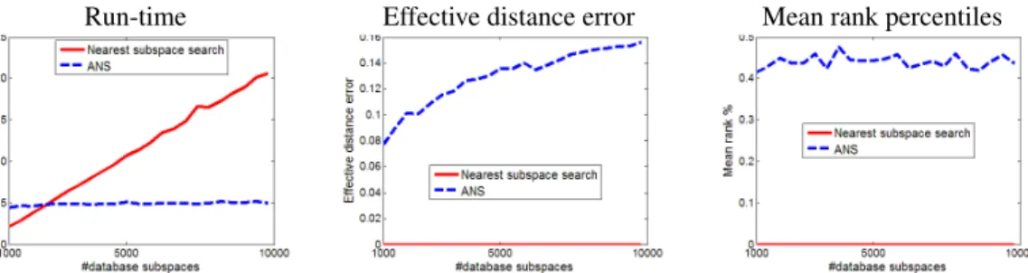
Run-time Effective distance error Mean rank percentiles
Figure 2.Varying database sizen.Comparing ANS with nearest subspace search, where ambient dimension isd= 60and intrinsic dimension isk= 4.
Run-time Effective distance error Mean rank percentiles
Figure 3.Varying ambient dimensiond. Comparing ANS with nearest subspace search, where database size isn= 5000and intrinsic dimension is k= 4.
. In particular, suppose we expect the nearest neighbor to lie at some distancetfrom a query, and denote byµt2+ν
the corresponding squared distance produced by our map-ping. Leta=ν/t2, then to obtain an approximation ratio
of1 +in the original spaceRdwe would need to select a ratio1 +0 ≈(1 +)/√µ+ain the mapped spaceRd0
, which can be very small particularly if we expect tto be small. Both issues can lead to a significant degradation in the performance of the nearest neighbor algorithm.
We would like to note further that whenk >1the non-zero constant offsetνis in fact inherent to our method. Us-ing simple arguments it can be shown that there exists no re-duction of the nearest subspace problem to nearest neighbor with points such thatν = 0, except for the trivial mapping. Specifically, ifν = 0any query point that is incident to a subspace, and consequently any two subspaces with non-trivial intersection, must be mapped to the same point. As there exists a chain of intersections between any two sub-spaces, the only possible mapping in the case thatν = 0is the trivial mapping.
We approach these problems by projecting the mapped database and query onto a space of lower dimension and applying nearest neighbor search to the projected points. Random projections are commonly used in ANN searches wheneverd logn. For a set ofnpoints, the celebrated Johnson-Lindenstrauss Lemma [12] guarantees with high probability that a random projection intoO(−2logn)
di-mension does not distort distances by more than a factor of
1 +. Magen [15] (see also [16]) has extended this Lemma
to affine spaces, showing that for a set ofnaffine spaces of rankk a random projection intoO(−3klog(kn))
dimen-sion distorts distances by no more than a factor of 1 +. Utilizing these results we can either first map the subspaces in the database to points and then project to a lower dimen-sional space which is logarithmic inn. Alternatively, we can first project the subspaces to a space of lower dimen-sion and then map the projected subspaces to points, this time obtaining a polylogarithmic dimension inn.
3.1. Algorithmic details
Given a database subspace we apply the mapping (2) if the subspace is linear, or (4) for affine subspaces. We then preprocess the database as required by our choice of ANN scheme (e.g., build kd-trees, or hash tables). Our prepro-cessing thus requires the same amount of space as would be used by the selected ANN method, on a database of points inO(d2).
Given a query our search proceeds by mapping it us-ing (2) or (4), based on a search for linear or affine sub-spaces. We then call our selected ANN method to report a database point near to our query. Our query running time is thusO(kd2) +T
AN N(n, d2), whereO(kd2)is the time required for mapping, andTAN N(n, d)is the running time for a choice of an ANN method (e.g., kd-trees, LSH), on a set ofnpoints inRd.
In the experiments reported below, we have found that good results can be obtained with significant speedup, if both the database and queries are first projected to a low
dimension, before mapping. We do this forNP projections each of dimensionb. On each random projection we extract
capproximate nearest neighbors. Finally, we compute the true distance between the query and allcNPcandidates, and report the closest match across all projections. Our overall query running time isNP(O(bd)+O(kb2)+TAN N(n, b2)+
cO(dk)), whereO(bd)is the time for projecting onto ab di-mensional subspace, andO(dk)the time for measuring the true distance between the query and a candidate database subspace.
4. Experiments
We applied our ANS scheme to both synthetic and real data. Run times were measured on a P4 2.8GHz PC with 2GB of RAM (thus, data was loaded to memory in its en-tirety). Our implementation is in C and uses the ANN kd-tree code of [2], with requested= 100. We expect similar results when using the LSH scheme. For all our matrix rou-tines we used the OpenCV library. For all our ANS experi-ments we chose to first project the data to randomly selected subspaces of dimensionb =k+ 1, and then map the pro-jected subspaces to points.
Synthetic data. Figs. 2 and 3 compare run-times and
quality of our ANS scheme and sequential subspace search. In Fig. 2 we vary the number of database subspaces, and in Fig. 3 the dimension d. Each test was performed three times with NQ = 1000 queries. For stability we report the median result. We usedNP = 23random projections measuring the true distance to the bestc= 15subspaces in each projection and reporting the best one.
Subspaces were selected uniformly, at random. Follow-ing [22], we generate queries such that at least one database subspace is at a distance of no more than(1 +)2Rp(d)
from each query, whereR= 0.1and= 0.0001.
Match quality was measured in two ways. First, the effective distance error [2, 13], defined as Err = (1/NQ)Pq(Dist
0/Dist∗−1), whereDist0is the distance
from queryqto the subspace selected by our algorithm, and
Dist∗ is the distance betweenq and its true nearest sub-space, computed off line. In addition, we present the mean rank percentile (MRP) for each query, measuring what per-centage of the database is closer to the query than the sub-space selected by our algorithm.
The results show that our algorithm is faster than sequen-tial database scan, while maintaining fairly lowErrrates. In addition, the MRP remains largely robust to the database sizen, increasing only moderately in larger dimensions.
Image approximation. We next demonstrate the use
of subspaces to represent local translations of intensity patches. Our goal here is to approximate the intensities of a query image by tiling it with intensity patches obtained from an image of an altogether different scene. A similar procedure is frequently used in the so called “by-example”
patch based methods for applications including segmenta-tion [6] and reconstrucsegmenta-tion [10].
A 1000 random coordinates were selected in a single im-age (Fig. 5). Then, 16 different, overlapping5×5patches around each coordinate were used to produce ak= 4 sub-space by taking their 4 principal components. These were stored in oursubspacedatabase. In addition, all 16 patches were stored for ourpoint(patch) database.
Given a novel test image we subdivided it into a grid of non-overlapping5×5patches. For each patch we searched the point database for a similar patch using (exact) sequen-tial and point ANN based search. The selected database patch was then used as an approximation to the original in-put patch. Similarly, we used both (exact) sequential and ANS searches to select a matching subspace in the subspace database for each patch. The point on the selected subspace, closest to the query patch, was then taken as its approxima-tion.
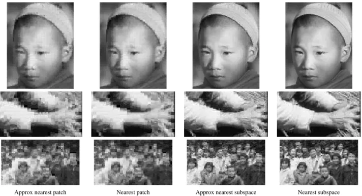
Fig. 4 presents the results obtained by each of the meth-ods. The full images and additional results are included in the supplemental material. Note the improved quality of the subspace based reconstructions over the point based meth-ods, evident also in the mean L1 error reported in Fig. 5. In addition, with the exception of the point ANN method, which did the worst in terms of quality, our ANS method was fastest, implying that an ANS method can be used to quickly and accurately capture local translations of image patches.
Yale faces. We tested the performance of our ANS
scheme on a face recognition task, using faces under vary-ing illumination. In our experiments we used the YaleB face database [9], with images scaled down by a factor of 10. We ran leave-one-out tests, taking one out of the 65 illumi-nations as a query, and using the rest to produce a database with intrinsic dimensionk= 9(following [4, 18]). With 10 subjects and 9 poses, the database is too small to provide the ANS method with a running time advantage over sequential scan (see Fig. 2). However, a comparison of the accuracy of the two methods is reported in Fig. 6. These results imply that although an approximate method makes more mistakes identifying the correct pose and subject, it is comparable to sequential search in detecting either the correct pose or subject.
Yale patches. Motivated by methods using patch data
for detection and recognition (e.g. [17]), we tested the ca-pabilities of the ANS method when searching for matching patches sampled from extremely different illumination con-ditions. For each subject+pose combination (90 altogether) in the YaleB database, we located 50 interest points. We then extracted, from all illuminations, the9×9patches cen-tered on each point. Patches from 19 roughly frontal illumi-nations, were then stored in apointdatabase, containing a total of90×50×19 = 85500patches. These same patches
Approx nearest patch Nearest patch Approx nearest subspace Nearest subspace
Figure 4.Image reconstruction results.Reconstructed using a single outdoor scene image. See Fig. 5 for run-times and error rates. Full images and more reconstructions included in the supplemental material.
Method Run time
Approx nearest patch 0.6 sec. Approx nearest subspace 1.2 sec. (Exact) Nearest subspace 4.2 sec. (Exact) Nearest patch 27.7 sec.
Figure 5.Image reconstruction details. From left to right, the single database image used for reconstruction, mean run times for each method, and L1 error reconstruction error. Both database and query images were taken from the Corel data set.
were further used to produce asubspacedatabase, contain-ing subspaces of dimensionk= 9, by taking the nine prin-cipal components of sets of corresponding 19 patches. A total of 4500 database subspaces were thus collected. Of the remaining illuminations, we took patches from the most extreme, to be our queries. Fig. 7 presents examples of illu-minations used to produce the database and queries.
We evaluate performance as the ability to locate a database item originating from the same semantic part as the query (e.g., eye, mouth etc.) We took a random selec-tion of 1000 query patches, all from the same pose. We then search both point and subspace databases for matches, using exact and approximate nearest neighbor (subspace) methods. Each database item matched with a query then votes for the location of the face center by computing
(cx, cy) = (qx, qy) + (dbdx, dbdy), where(cx, cy)is the es-timated center of mass,(qx, qy)is the position of the query
and (dbdx, dbdy) is the position of the selected database item, relative to its image’s center (using cropped images, where the face center is located in the center of the image). The vote histograms computed by each method are pre-sented in Fig. 7. Under the extreme lighting conditions used, point based methods failed completely since there are no good near neighbors in the data. Both subspace methods managed to locate the correct center of mass, where exact scan did significantly better, but at a higher running time.
5. Conclusion
The advantages of subspaces in pattern recognition and machine vision have been demonstrated time and again. In this paper we have presented a method which facilitates har-nessing subspaces, and extending their use to applications involving large scale databases of high dimensions. To this end we have provided an algorithm for sub-linear
approx-Wrong nearest neighbor Wrong person Wrong person AND pose
Figure 6.Faces under varying illumination. Comparison of face recognition results on the Yale-B face database [9] between exact nearest subspace search and the proposed approximate search. (Left) The approximated search has more errors than exact search. (Middle) The number of times a wrong person was detected by ANS is small and shows that in many cases the nearest neighbor returned by ANS is of the same person in a wrong pose. (Right) In other cases a different person in the correct pose was detected. The frequency at which both the wrong person and the wrong pose were detected is comparable to that of exact search.
Database Query
(a) (b) (c)
Figure 7. Yale patches. (a) Two examples of images used for the databases. (b) Two examples of images used for query patches. Queries were produced from images under extreme illuminations, simulating dif-ficult viewing conditions. (c) Histograms of face-center votes by each se-lected database item. From top to bottom: Nearest subspace, our ANS method, and nearest patch. These demonstrate the number of times the correctsemanticitem (e.g., eye, mouth) was selected from the database by each method. Run-times were 16.3 seconds for exact subspace search, 11.0 seconds for our ANS method, and 9.2 seconds for the point search.
imate nearest subspace search. Our goal is now to fur-ther this study, by investigating different applications which might benefit from these improvement in quality and speed.
References
[1] P.K. Agarwal, J. Erickson, “Geometric range searching and its rela-tives,”Contemporary Mathematics,223: 1–56, 1999.
[2] S. Arya, D. Mount, N. Netanyahu, R. Silverman, A. Wu. “An opti-mal algorithm for approximate nearest neighbor searching in fixed dimensions,”Journal of the ACM,45(6): 891–923, 1998. Source code available from www.cs.umd.edu/ mount/ANN/.
[3] J.J Atick, P.A. Griffin, A.N. Redlich, “Statistical Approach to Shape from Shading: Reconstruction of Three-Dimensional Face Surfaces from Single Two- Dimensional Images,”Neural Computation,8(6): 1321-1340, 1996.
[4] R. Basri, D. Jacobs, “Lambertian reflectances and linear subspaces,”
IEEE TPAMI,25(2): 218–233, 2003.
[5] V. Blanz, T. Vetter, “Face Recognition based on Fitting a 3D Mor-phable Model,”IEEE TPAMI,25(9): 1063–1074, 2003.
[6] E. Borenstein, S. Ullman, “Learning to Segment,” ECCV,3023: 315–328, 2004.
[7] M.E. Brand, “Morphable 3D models from video,”CVPR,2: 456–463, 2001.
[8] M. Datar, N. Immorlica P. Indyk, V. Mirrokni, “Locality-sensitive hashing scheme based on p-stable distributions,”SCG ’04: Proceed-ings of the twentieth annual symposium on Computational geometry: 253–262, 2004.
[9] A.S. Georghiades, P.N. Belhumeur, and D.J. Kriegman, “From few to many: illumination cone models for face recognition under variable lighting and pose,”IEEE TPAMI,23(6): 643–660, 2001.
[10] T. Hassner, R. Basri, “Example based 3D reconstruction from single 2D images,” InBeyond Patches workshop, CVPR., 2006.
[11] P. Indyk, R. Motwani, “Approximate nearest neighbors: towards re-moving the curse of dimensionality,” InSTOC’98: 604–613, 1998. [12] W. Johnson, J. Lindenstrauss, “Extensions of Lipschhitz maps into a
Hilbert space,”Contemporary Math: 189–206,26, 1984.
[13] T. Liu, A.W. Moore, A. Gray, K. Yang, “An Investigation of Practical Approximate Nearest Neighbor Algorithms,”NIPS: 825–832, 2004. [14] S. Meiser, “Point location in arrangements of hyperplanes,”
Informa-tion and ComputaInforma-tion,106: 286–303, 1993.
[15] A. Magen, “Dimensionality reductions that preserve volumes and distance to ane spaces, and their algorithmic applications”, Random-ization and approximation techniques in computer science. Lecture Notes in Comput. Sci.,2483: 239–253, 2002.
[16] A. Naor, P. Indyk, “Nearest neighbor preserving embeddings,”,ACM Transactions on Algorithms, forthcoming.
[17] L. Fei-Fei, R. Fergus, P. Perona, “One-Shot Learning of Object Cat-egories.”IEEE TPAMI,28(4): 594–611, 2006.
[18] R. Ramamoorthi, P. Hanrahan, “On the relationship between radi-ance and irradiradi-ance: determining the illumination from images of convex Lambertian object.”Journal of the Optical Society of Amer-ica,18(10): 2448–2459, 2001.
[19] C. Tomasi, T. Kanade, “Shape and Motion from Image Streams under Orthography: A Factorization Method,”IJCV,9(2): 137–154, 1992. [20] L. Torresani, D. Yang, G. Alexander, C. Bregler, “Tracking and Mod-eling Non-Rigid Objects with Rank Constraints,”CVPR: 493–500, 2001.
[21] S. Ullman, R. Basri, “Recognition by Linear Combinations of Mod-els,”IEEE TPAMI,13(10): 992–1007, 1991.
[22] P.N. Yianilos, “Locally lifting the curse of dimensionality for nearest neighbor search (extended abstract),”Symposium on Discrete Algo-rithms: 361–370, 2000.
![Figure 6. Faces under varying illumination. Comparison of face recognition results on the Yale-B face database [9] between exact nearest subspace search and the proposed approximate search](https://thumb-us.123doks.com/thumbv2/123dok_us/802068.2601374/8.918.144.748.108.273/figure-illumination-comparison-recognition-database-subspace-proposed-approximate.webp)
