DOI 10.1007/s00530-015-0479-0
SPECIAL ISSUE PAPER
Uncertainty‑aware estimation of population abundance using
machine learning
Bastiaan J. Boom1 · Emma Beauxis‑Aussalet2 · Lynda Hardman2 · Robert B. Fisher1
Published online: 3 September 2015 © Springer-Verlag Berlin Heidelberg 2015
1 Introduction
We introduce a method to improve counting of elements in classes based on the scores given by machine learn-ing. It addresses user needs for evaluating interclass confusions and their potential biases (e.g., a large class overwhelms a smaller class with False Positives). For instance, video monitoring of fish populations can com-pare species abundance, or cell recognition can evaluate concentrations of blood cells. In these cases, users need accurate counts of elements per class, with limited inter-class confusions (e.g., systematically inter-classifying elements in the same wrong class). Our method addresses this need beyond the usual methods determining optimal selection thresholds in the parameter settings. Thresholds are usu-ally set on a single parameter, e.g., a similarity score, representing the similarity (e.g., a distance or likelihood ratio) between a candidate element and a class model. The threshold is chosen to balance type I and II errors [i.e., False Positive (FP), False Negative (FN)] depending on use cases. Our method does not discard elements below a threshold. It uses all elements and similarity scores to estimate interclass confusions, and obtain probabilities of class membership. These probabilities can provide more accurate counts of elements per class, by weighting ele-ments given their similarity scores. Our method is par-ticularly robust to unbalanced groundtruth that under- or over-represents some classes. We do not claim to classify individuals more accurately. Rather, we claim that the use
of similarity scores of groundtruth samples, when applied
to modeling the probability of class membership, allows more accurate estimate of the true counts of individuals per class.
Furthermore, we address uncertainty issues with data visualization. Machine learning errors are usually
Abstract Machine learning is widely used for mining
collections, such as images, sounds, or texts, by classify-ing their elements into categories. Automatic classification based on supervised learning requires groundtruth datasets for modeling the elements to classify, and for testing the quality of the classification. Because collecting groundtruth is tedious, a method for estimating the potential errors in large datasets based on limited groundtruth is needed. We propose a method that improves classification quality by using limited groundtruth data to extrapolate the potential errors in larger datasets. It significantly improves the count-ing of elements per class. We further propose visualization designs for understanding and evaluating the classifica-tion uncertainty. They support end-users in considering the impact of potential misclassifications for interpreting the classification output. This work was developed to address the needs of ecologists studying fish population abundance using computer vision, but generalizes to a larger range of applications. Our method is largely applicable for a variety of Machine learning technologies, and our visualizations further support their transfer to end-users.
Keywords Supervised machine learning · Uncertainty
visualization · Logistic regression
* Emma Beauxis-Aussalet
[email protected] Bastiaan J. Boom [email protected]
1 University of Edinburgh, Edinburgh, UK 2 CWI, Amsterdam, The Netherlands
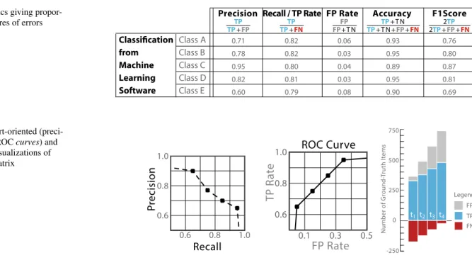
visualized with graphs such as ROC and Precision/Recall curves, or measures such as F1 score (Figs. 1, 2). These do not differentiate noise from potential biases due to interclass confusion. They typically support the choice of parameter thresholds, which is not relevant for our method. Finally, they are tedious to understand for non-expert users who need to evaluate the classification uncertainty. Hence we developed visualization designs addressing user needs for evaluating interclass confusions, and supporting non-experts in understanding uncertainty. Our contributions are two-fold:
Estimation of classification biases We specify a method
applying logistic regression on similarity scores (i.e., simi-larity of elements with class models). It is applicable for both two-class and multi-class problems. It estimates the probability of confusing classes, and the biases due to the similarity of classes’ elements (i.e., given their
similar-ity scores). The biases estimation is used to significantly
improve the task of counting elements in each class.
Visualization of biases due to interclass confusions We
specify user requirements for estimating and visualizing classification uncertainty. We design original visualizations supporting both the understanding of the classification method, and the evaluation of interclass confusions. They provide non-expert users with accessible descriptions of the biases due to systematic misclassifications.
2 Related work
Counting individuals, and classifying them into catego-ries, is a basic task for a variety of studies. For instance,
ecologists largely study population abundance for dif-ferent organisms, which is based on classifying the spe-cies of individuals [10]. Machine learning algorithms can automate classification, and is cost- and time-effective. However, classification uncertainty is a major issue for the uptake of such technologies. Likewise the visualiza-tion community identifies uncertainty as a major challenge [8, 9, 16]. Uncertainty needs to be considered along with the data transformation steps, and the machine learning components are typically concerned. As an example, com-puter vision was applied for marine ecology, and its reli-ability compared to other techniques [4, 12, 15, 28–30]. In the ecology domain, the main approach to deal with uncer-tainty consists of repeating measurements and applying statistical techniques (e.g., ANOVA) [24, 25]. Only [4, 12] used evaluation methods specific to the applied computer vision techniques. This gap between ecology and computer vision practices highlights the need for handling, explain-ing and visualizexplain-ing potential misclassifications.
Several methods have been developed to automati-cally estimate counts of objects, mostly from image data. In this case, approaches can be divided according to [20] into feature-, score- and decision-level algorithms. In [11,
17], the estimation of automatic land cover categories is improved based on the confusion matrix, where these papers use a confusion matrix (decision-level) determined from groundtruth to correct the under and overestimates. In computer vision, counting cells [19] and crowds [7] is often performed using regression on the image features, which achieve very accurate counts (feature level). By performing the count on features, in the case of cells, a single cell is not identified with these kind of methods, but by looking at the Fig. 1 Metrics giving
propor-tional measures of errors PrecisionTP
TP+FP Recall / TP Rate TP TP+FN FP Rate FP FP+T N Accuracy TP+T N TP+T N +FP+FN F1Score 2TP 2TP+FP+FN 0.71 0.82 0.06 0.93 0.76 0.78 0.82 0.03 0.95 0.80 0.95 0.80 0.04 0.89 0.87 0.82 0.81 0.03 0.95 0.81 0.60 0.79 0.08 0.90 0.69 Classification Class A from Class B Machine Class C Learning Class D Software Class E
Fig. 2 Expert-oriented (preci-sion/recall, ROC curves) and simplified visualizations of confusion matrix 0.6 0.8 1.0 0.6 0.8 1.0 Pre cisio n Recall 0.1 0.3 0.5 0.6 0.8 1.0 TP Ra te FP Rate ROC Curve 0 250 500 750 -250 FN FP Legend: TP Number of Ground-Truth It em s t1 t2 t3 t4
higher level features like color, edges, etc., these methods give a direct estimate of the count. In the case of crowds [7], this has privacy advantages because their method does not directly recognise a single individual, which will give us privacy sensitive information. Often machine learn-ing methods for findlearn-ing or identifylearn-ing a slearn-ingle individual object are available, but the feature level approach in this case does not use this information. Finally, there are only a few papers that tackle the problem of biased estimation of a classifier. In [26], bias correction is based on the estimated decisions of the classifier. While in [23], authors estimate the a priori distribution of a new dataset based on the fea-tures. The main difference with previous approaches is that we use the similarity scores from automatic classification methods to determine the counts, while previous meth-ods work either directly at the decision level (having less information) or at the feature level (can not use classifier output).
Common metrics evaluating misclassifications are based on confusion matrices (Fig. 3). Uncertainty visualizations commonly use pairs of metrics (e.g., Precision/Recall, ROC curves with TP and FP rates), computed for different
similarity score thresholds. They are typically complicated
for non-experts, and likely to be overwhelming or mislead-ing [3]. Non-experts may not identify the aspects of uncer-tainty revealed, or concealed, by expert visualizations. [5] provides a first attempt to simplify the visualization of confusion matrices and address the needs novices (Fig. 2). Other approaches such as [1] address expert usages and parameter setting tasks, without addressing end-user inter-pretation of classifiers’ end-results.
3 Biases‑aware classification method
We introduce a method for estimating the probabilities of classification errors, and use these probabilities to correct biases in counting tasks. Counting typically con-sists in estimating the numbers of elements belonging to each class. In tasks such as population monitoring, users particularly require estimates of interclass confu-sions. They need to know which species are often con-fused with one another [2], because they ultimately need to evaluate the potential biases in counts of individuals
in each class. By computing the probabilities, we do not improve the recognition performance but obtain a statis-tical estimate of bias given a large dataset. Compared to common methods based on thresholding, this method is able to estimate and correct biases due to interclass con-fusions. Here, we introduce a method providing accurate biases estimations, improving the counting of elements in each class, and addressing end-user needs for uncer-tainty evaluation.
3.1 Comparison with methods based on thresholding
Classification methods use groundtruth sets (i.e., collec-tions of manually classified elements) for (1) training
models of classes’ elements, using features measured amongst examples (e.g., shape, color, size of objects);
(2) validations, to refine models’ parameters and (3)
testing the quality of the classification results. The
lat-ter two (e.g., the validation and test sets) are used in a innovative approach to provide the counts. Elements of
the validation and test set are compared to class models
using descriptive features, such as shape or color in com-puter vision. The closeness of their feature values is usu-ally synthesized in a single metric by a classifier. Such metric is referred here as a similarity score si,c, for an
item i, a candidate class c, yielding a class membership yi,c = {0, 1}. The higher a score, the more likely elements belong to a class. But the likelihood of class membership is not itself evaluated. Boolean class membership is usu-ally decided by setting thresholds on similarity scores
(i.e., yi,c= 1 if si,c>tc). Our counting method introduces
an original use of all similarity scores without requiring a threshold setting.
The choice of threshold depends on the machine learn-ing method, where t=0 is a natural choice for Adaboost
and log-likelihood ratios. Thresholds are usually optimized using ROC or Precision/Recall curves to balance type I and II errors. For instance, ROC curves can be use to limit FP rate against FN rate, if appropriate. A threshold’s effect on counting tasks is ambiguous: e.g., thresholds optimal for a training set may bias the classification of the test set. In the multiclass case, thresholds are not necessary for cases where items are classified in the class for which they have the highest similarity score.
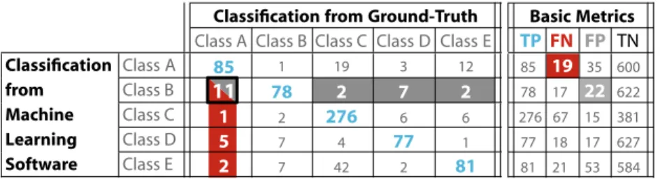
Fig. 3 Example of confusion matrix, and counts of True Positive TP, False Negative FN, False Positive FP, True Nega-tive TN
Classification from Ground-Truth Class A Class B Class C Class D Class E
Classification Class A 85 1 19 3 12 from Class B 11 78 2 7 2 Machine Class C 1 2 276 6 6 Learning Class D 5 7 4 77 1 Software Class E 2 7 42 2 81 Basic Metrics TP FN FP TN 85 19 35 600 78 17 22 622 276 67 15 381 77 18 17 627 81 21 53 584
3.2 Original counting method based on logistic regression
Logistic Regression is able to compute the probability of cor-rect and incorcor-rect classification of items given their similar-ity scores, by estimating the error distribution over the scores (observed in the validation set) for a potentially unbalanced groundtruth. This technique is very similar to Platt scaling [22] except that we assume similarity scores as input instead of adding a normalisation function to the classifier to compute the probability. We explain this new method first for the two class problem and afterwards for the multiclass problems.
3.2.1 Two class problem
Logistic Regression computes the probability P(yi|si) that item i belongs to a given label yi= {0, 1}. This depends on
the similarity score si from the classifier which indicates
how item i is similar to the positive class. Logistic Regres-sion is able to translate the similarity scores si, which can
be in any range, to a probability. This is achieved by the following calculation:
The unknown parameters β0, β1 in Eq. (1) need to be com-puted based on a validation set. This validation set should be randomly sampled from the test set for which we would like to obtain the final count. However, the validation set should have groundtruth labels, which are unknown on the final test set. The parameters β0, β1 allow to describe a function that
extrapolate the counts learned on the validation set to the test set. These parameters can be calculated by most statis-tical software packages, by using the maximum likelihood estimation that finds the parameters for which the probabil-ity on the validation data is best. In [21], the maximum like-lihood estimation is performed using an iterative weighted least-squares method, because there is no close-form solu-tion to compute the parameters β. The iterative weighted
least-squares method proposed in [21] is equivalent to the Newton-Raphson method for finding the optimal value of the likelihood function. In our explanation of Logistic Regression we used the “logit” kernel, however our experi-ments gave very similar results for both the logit kernel and the probit kernel [6]. Based on the input score and labels, this function searches for the optimal parameters β that fit
the labels. The estimated final count of positive items, for all N items i in the test set, is given by Ey =iN=1P(yi|si).
3.2.2 Multiclass problem
The multiclass problem can be seen as very simi-lar to the two class problem, where each multiclass
(1)
P(yi|si)=
1 1+e−(β0+β1si)
problem can be converted into a two class problem. Instead of having a label that can have multiple outcomes
yi= {0, 1, 2, 3,. . .,M}, we use a binary label yi,c= {0, 1}
indicating whether item i belongs to class c (i.e., yi,c=1) or does not belong to that class (i.e., yi,c=0). For the mul-ticlass problem, instead of having a single score, we have for each class a score si,c. It might be counterintuitive that
we do not have two scores for the two class problem. But the scores indicate the similarity towards a certain class with respect to another class. For the two class problem one score suffices. But for an M class problem, for every class, we need a score indicating whether items do not belong to all other classes, which results in M scores. Given a set of groundtruth labels yi,c = {0, 1} and scores si,c, for
improv-ing item counts for one class, we could use only the scores indicating similarity to that class (e.g., si,c1 for class 1). In this case, Eq. (1) is sufficient. However, the scores for all other classes provide additional information, and better results can be obtained with the following equation:
This equation estimates the probability that item i belongs to a class c given the similarity scores for all classes
ζ = {c1,. . .,cM}. We calculate for each class a different
parameter vector β using Logistic Regression. For each
item i we obtain M probabilities of class membership, i.e., one for each of the M classes. The M probabilities are com-puted using the same set of scores si,ζ, but different
param-eter vectors β. A problem with this approach is that we can
not guarantee that the M probabilities for a single item will sum to one. This is possible if we use multinomial logis-tic regression. The large amount of data made multinomial logistic regression not usable for our problem where the estimation of the parameters β for the multinomial case
could not be found in a reasonable time frame (under a day). The approach described here already provides accu-rate count, especially because of the large amount of data used for the estimation, where normalizing the probabilities based on a single item did not work. The final count for a certain class c is obtain by the sum of the probabilities for each item Ey,c=Ni=1P(yi,c|si,c).
3.3 Sampling strategy
To estimate the counts over a given dataset, the sampling strategy for collecting groundtruth sets is of vital impor-tance. This work assumes the following sampling strategy: Given the entire dataset, we select two subsets, one for
training and one for validation, to estimate item’s counts
for the remaining data (considered as the test set). For
training and validation sets, we obtain groundtruth
infor-mation by manual annotation. The training set allows to (2) P yi,c|si,ζ= 1 1+e− β0,c+β1,csi,c1+···βM,csi,cM
train a classifier (using any machine learning method). This set does not have to be a representative subset of the entire dataset. It might be even better to balance the classes for better recognition performance. The validation set is used to verify the performance of the classifier on untrained examples. It is of vital importance that this set is represent-ative of the test set, i.e., the distribution of items amongst classes and similarity scores need to be similar to that of
the test set. This can be achieved by random sampling.
Based on the scores for the correct (TP, TN) and erroneous (FP, FN) classifications performed on the validation set, our method estimates the counts in the test set.
4 Evaluation of the counting method
We evaluate the performance of our counting method for 3 counting tasks, with binary and multiclass problems. We evaluate the accuracy of counts based on logistic regres-sion, compared to the results of thresholding methods. Finally, we evaluate the estimated values (FP, FN, etc.) from logistic regression to compute the visualizations.
4.1 Experimental datasets
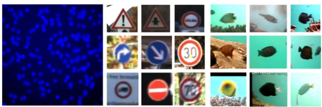
Real-world groundtruth sets are often unbalanced, which significantly impacts on machine learning performances. The datasets are chosen to demonstrate our approach, and its robustness to good and bad classification results and bal-anced and unbalbal-anced datasets. Figure 4 gives examples of the datasets’ elements.
Cell images (binary classification) The task is to count cells in each image. The experimental dataset is produced with a simulation program [18]. It is very unbalanced due to scarce positive examples. The groundtruth consists of 16 images for training and validation and 16 for testing. Two simple classifiers based on circular features [i.e., linear dis-criminative analysis (LDA) and Adaboost] are trained on this dataset.
Traffic signs (multiclass problem) The task is to count
traffic signs (Fig. 4; [13]). 43 Classes of traffic signs need to be recognized. The machine learning algorithm extracts
color dense SIFT features on which k mean clustering is applied. The feature vectors are processed with both Ada-boost and SVM techniques. The original training set is ran-domly split into training and validation sets, the obtained results are over 20 random runs where we use the original 22,011 item testset.
Fish images (multi-class problem) The task is to count
fish from 12 species in the collection described in [14]. A hierarchical SVM classifier was specifically designed for this problem. In the experiment, the data is 20 times ran-domly divided into a validation and test set. This data was not used to create the fish model.
4.2 Impact on counting tasks
The goal of this research is not to improve the recogni-tion results of classifiers, although better classifiers can be used for some of the problems. The goal of this research is however to exploit the large amount of data to estimate the underlining statistics like the counts per class, even in case of “error-prone” classifiers. Section 3.1 shows that the decision depends on a threshold t, where for the classifi-ers Adaboost and LDA (which uses a log-likelihood ratio)
t=0 is a natural choice. Due to the large imbalance in
the cell dataset, with images of 256×256 containing only
around the 150 cells, it is difficult for a classifier to perform well. Logistic regression does not improve the performance after running it on the similarity score. However it gives probabilities that are representative for the expected perfor-mance. Given these probabilities, the expected count can be estimated accurately as is shown in Table 1, even for bad classifiers.
For the multiclass problems, we experimented with two strategies to set the thresholds. The first strategy is simi-lar to the cell example where in the case of Adaboost the threshold is set to t=0. The second strategy is to use the
class with the maximum score for a given element, which is done for both Adaboost and SVM. Although the sec-ond strategy seems to perform better when estimating the counts, as can be observed from Table 1, it might depend very much on the automatic classifier used. The perfor-mance of SVM in Table 1 shows that this classifier already Fig. 4 The datasets used for
evaluation: images of cells, traf-fic signs and fish
works very well, although it was biased towards a couple of classes, which is the reason why our estimate of the counts are better still.
For the fish species recognition dataset, the outputs of a classifier specifically designed for this problem are used on a new dataset. The set of fish species is unbalanced, e.g., obtaining enough examples of rare species was a challenge. By running the fish recognition on new videos, we discov-ered that although the recognition methods have good rec-ognition rates, the classifier is biased toward certain classes
and underestimates the amounts of false positives from the detection stage. The correction based on logistic regression is able to correct this where the final errors in estimated counts are much smaller (see Table 1).
4.3 Uncertainty of the counting method
To create the visualization especially in the multi-class cases, not only is it important that the final count is cor-rectly estimated, but also the other information in the
0 5 10 15 20 25 30
FN for two closest classes FP for two closest classes FN FP count
Average absolute error ofLogistic Regression
FN for all other classes FP for all other classes
0 2 4 6 8 10 12 14 16
FN for two closest classes FP for two closest classes FN FP count
Percentage of error given of Logistic Regression given counts per class
FN for all other classes FP for all other classes
0 5 10 15 20 25 30
FN for two closest classes FP for two closest classes FN FP count
FN for all other classes FP for all other classes
Average absolute error ofLogistic Regression
0 2 4 6 8 10 12 14 16
FN for two closest classes FP for two closest classes FN FP count
FN for all other classes FP for all other classes
Percentage of error given of Logistic Regression given counts per class
Traffic sign: (a) Numbers of errors with Adaboost (b) Percentage of error with Adaboost
Traffic sign: (c) Numbers of errors with SVM
Fish: (e) Numbers of errors with Hierarchical SVM
(d) Percentage of error with SVM
(f) Percentage of error with Hierarchical SVM
0 5 10 15 20 25 30
FN for all other classes FP for all other classes FN for two closest classes FP for two closest classes FN FP count
Average absolute error of Logistic Regression
0 5 10 15
FN for two closest classes FP for two closest classes FN FP count
FN for all other classes FP for all other classes
Percentage of error given of Logistic Regression given counts per class
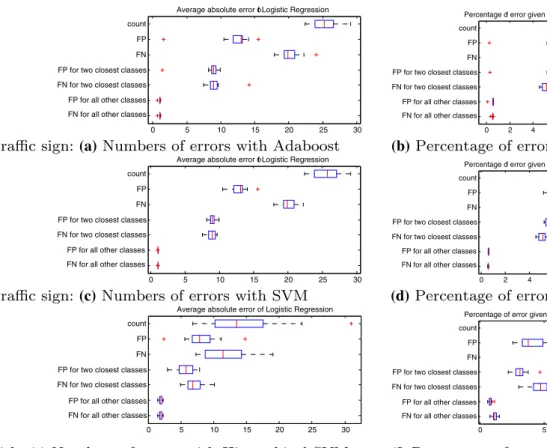
Fig. 5 Average errors over 20 cross-validations estimating: overall counts (TP + FP), total counts of FP and FN, counts of FP and FN for the two most similar classes only, average
counts of FP and FN for all other classes (i.e., for all classes
cj in ζ= {c1,. . .,cM},M1 Mj=1FPζ→cj/(TPcj+FPζ→cj) and
1 M
M
j=1FNcj→ζ/(TPcj+FNcj→ζ) are used for (a), (c) and (e))
Table 1 Error in counts for the different datasets, showing that our approach is able to correct errors based on the similarity scores from other machine learning methods and works significantly better in all cases
The standard deviation is estimated over 20 cross-validation folds
Dataset Machine learning Error in counts
Normal Corrected
Cell Adaboost 2075.7 (±444.7) 11.86 (±1.26)
65536 examples (average 180 positives) LDA 1910.2 (±997.0) 11.13 (±2.66)
Traffic signs Adaboost (threshold) 3146.3 (±155.91) 23.38 (±1.92)
12630 examples Adaboost (max score) 521.50 (±19.35) 23.38 (±1.92)
SVM (max score) 31.92 (±1.92) 25.40 (±2.00)
Fish Hierarchical SVM 693.74 (±5.96) 13.05 (±3.44)
graphs should be correct. More specifically, it is also important to know how well the estimations for the False Positives and False Negative are on three levels, namely:
overall estimation given the rest of the classes, estimation
for the two most similar classes which thus bring most uncertainty, and finally the estimation for all the classes. Figure 5 shows the error of our estimates with respect to these three levels, in both absolute numbers and in percent-ages given the true counts for each class. This figure shows that the estimates by our logistic regression are not perfect, which can be expected given that they are statistical esti-mates, but that the errors are in an acceptable range allow-ing the user to get a feelallow-ing of what kind of errors to expect from the machine learning methods. The errors for the two
most similar classes (the classes with which a particular
class is most confused) are around 5–10 %, while the error for all the classes is around 1 %. For classes that are easy to separate, the method is able to predict more accurately that these classes do not belong to a certain class. In Fig. 5, we can also observe that the results over different data-sets and classifiers are similar, showing the stability of the methodology.
5 Visualization of classification biases
User understanding of classification errors is crucial for trusting classification systems, and for successful technol-ogy transfer. Hence we developed visualizations addressing the needs of non-expert users for estimating interclass con-fusions. We provide both explanations of the classification method, a basic requirement for understanding uncertainty, and evaluations of potential biases in end-results.
5.1 Explaining the classification method
Developing user acceptance of complex machine learning solutions is a difficult task for technology suppliers. For end-users, their solutions often appear as opaque compo-nents which underlying technology is hardly verifiable (i.e., a black box). User-friendly explanations can help to develop a dialogue with potential users, to build informed trust from uninformed skepticism. Hence we designed explanatory visualizations of the step-by-step procedure of our logistic regression method. They describe the under-lying principles of the machine learning processes, and empower users with accessible system knowledge.
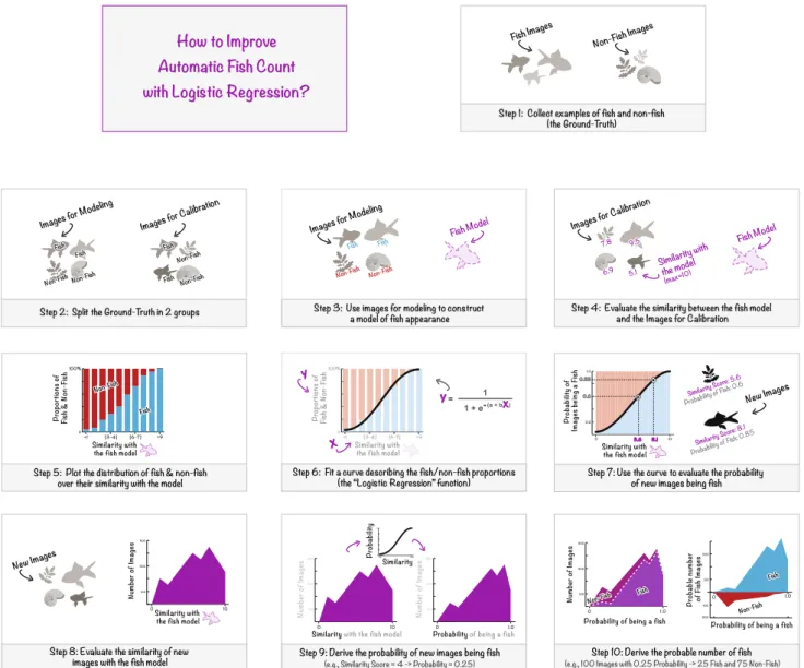
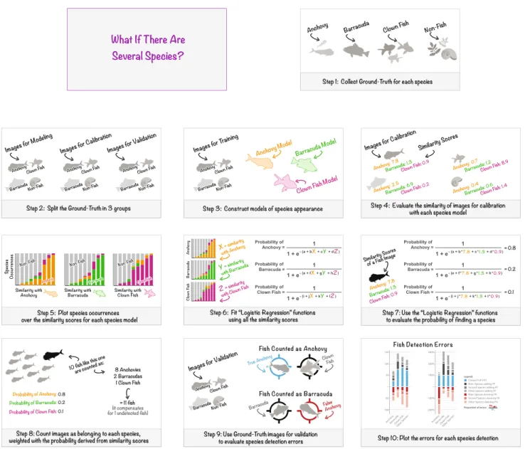
We designed 2 explanatory visualizations. The first explains logistic regression for binary classification (Fig. 6). The second extends its application to multiclass problems (Fig. 7). Their narrative comic strip-like approach, with user-friendly fonts and simple phrasing, aims at rendering the technical content more welcoming and accessible. We
collected informal feedback from potential users of our system. The comic-strip style was welcomed. The explana-tions were found engaging and encouraged users to explore the complexity of machine learning uncertainty.
The main issue concerned the tradeoff between intro-ducing technical terms, and vulgarizing logistic regression theory. Technical terms that can be avoided are replaced with common vocabulary, to make explanations more accessible. But for a user who was familiar with logistic regression, common vocabulary was confusing, and techni-cal terms were preferred. Further, semantic gaps can occur between the terms most commonly used by either technol-ogy or domain experts. It can lead to confusions and mis-understandings. For instance, biologists commonly refer to
calibration and validation sets of groundtruth, which are
usually called validation and test sets in computer vision, respectively. Hence, to develop the dialogue between users and technology suppliers, unfamiliar users should learn the appropriate technical terminology, and conversely, technol-ogy suppliers should learn the terms used in the applica-tion domain. Thus we recommend that explanatory visuali-zations are customized for the application domain so as to introduce both terminologies and their correspondences.
Finally, we observed the need for an additional tuto-rial explaining the process of groundtruth evaluation, prior to describing logistic regression. Users required more information regarding: the groundtruth collection proce-dure (e.g., annotator profiles, levels of agreement), the construction of class models (e.g., features used to train algorithms), and the initial errors observed before logistic regression (e.g., groundtruth evaluation using similarity score thresholds).
5.2 Visualizing interclass confusions
Uncertainty due to misclassification is measured using groundtruth evaluations. Error measurements are encoded in confusion matrices (Fig. 3). All possible interclass con-fusions are encoded in terms of misclassifications between pairs of classes. Confusion matrices indicate how many FN were missed for one class and erroneously attributed to another class as FP. The counts of misclassifications are given for all pairs of classes. The information on mis-classification errors is complete, however it is complex to visualize.
We simplified the visualization of interclass confusion as shown in Figs. 8, 9. We use three simple visual con-cepts: Missed items (FN) in red below the zero line,
Cor-rect items (TP) in blue above the zero line, and Added
items in grey and stacked on top of TP. The design intends
to be more tangible than ROC or Precision/Recall curves. The multiple interclass confusions are synthesized with a limited level of detail. For each class, the main sources of
confusion are indicated. We select the 2 classes yielding the most FP and FN, and display the magnitude of errors they imply. Errors remaining for other classes are dis-played together in one block. Details of the errors impact-ing one class are provided when users select a class of interest (Fig. 9, bottom).
Our design addresses 5 issues with confusion matri-ces: (1) error interdependence, as FN for one class are FP for another; (2) multiplicity of pairwise confusions, i.e., with n classes, a total of n(n− 1) interclass confu-sions are measured; (3) relative error magnitude in unbal-anced groundtruth (i.e., scarcity or excess of groundtruth for some classes), or in end-results (i.e., containing larger and smaller classes); (4) considering type I and II errors in accordance to application requirements; (5) complexity of uncertainty metrics, which is potentially misleading.
Error interdependence Users need to identify which
classes are likely to be confused with another, as FN for one class are FP for another. For instance, in Fig. 3 the cell with a black contour indicates both 11 FN missed for Class A, and 11 FP added to Class B. Hence confusion matrices need to be read both column- and row-wise. This demands a high cognitive load (e.g., to memorize all cell values and their semantics), which is error prone (e.g., users may read only columns or rows, or forget cell values and semantics). The number of cells to read is usually reduced by cumulat-ing misclassifications for each class. Figure 3 illustrates the synthesis of FN (column with red background) and FP (row with grey background). However, with this synthesis users can no longer identify which classes are likely to be con-fused with another, and this information is required for esti-mating potential biases in end-results. E.g., a large increase Fig. 6 User-friendly explanations of logistic regression for binary classification
Barracuda Anch ovy Clown Fish Other Specie s 100% 200% 300% -200% -100% Barracuda Anch ovy Clown Fish Other Specie s 50 100 150 -100 -50
Main Species drawing FN Second Species drawing FN Other Species drawing FN Second Species adding FP Correct Fish (TP)
Legend:
Proportion of errors:
Main Species adding FP Other Species adding FP
FNa b
TPa
Fig. 7 User-friendly explanations of logistic regression for multiclass classification
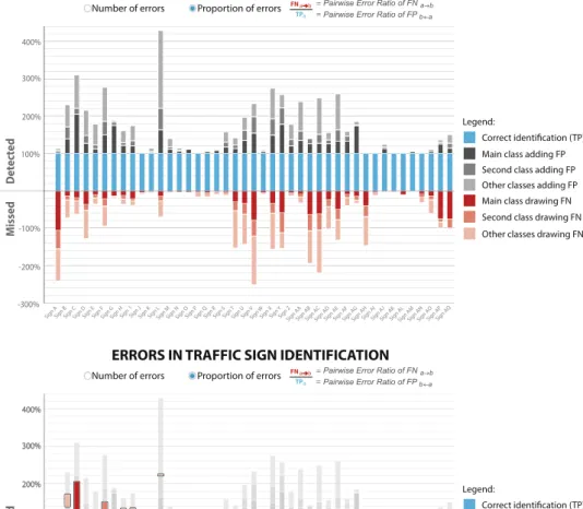
Fig. 8 Visualization of inter-class confusions using numbers of TP, FP and FN -400 -200 200 400 600 800 Detec te d Missed
ERRORS IN TRAFFIC SIGN IDENTIFICATION
Number of errors Proportion of errors
Sign B Sign C Sign A Sign D Sign N Sign M Sign L Sign K Sign J Sign I Sign H Sign G Sign F Sign E Sign O Sign Q Sign R Sign P Sign S Sign AC Sign AB Sign AA Sign Z Sign Y Sign X Sign W Sign V Sign U Sign T
Sign AD Sign AFSign AG Sign AHSign AI Sign AE Sign Sign AK
AJ Sign AQ Sign AP Sign AO Sign AN Sign A M Sign AL
Main class drawing FN Second class drawing FN Other classes drawing FN Second class adding FP Correct identification (TP) Legend:
Main class adding FP
Other classes adding FP
= = FNa b
of one class implies an increase of its FN, and can thus induce a deceptive increase of other classes. To address this issue, we recommend not to synthesize all errors in accu-mulated numbers of FP and FN, so as to preserve the neces-sary information originally encoded in confusion matrices.
Multiple pairwise confusions Numerous confusions
between 2 classes need to be visualized. This can easily clutter visualizations and overwhelm users. Hence, we rec-ommend to select the most important pairwise confusions, and to synthesize the remaining errors. For each class, we select the 2 classes receiving the most FN, and the 2 classes from which most FP are originated. The remaining errors are accumulated.
Unbalanced datasets The proportions of items per class
can greatly vary within groundtruth sets, and within sets of end-results. In this case, basic (TP, FN, FP, TN) and
advanced metrics can be misleading. The magnitude of FP is dependent on the magnitude of their original classes, i.e., the larger a class the more FP it yields for other classes. A small class can be overwhelmed by FP from a larger class, whereas few FN are missed. Inversely, a large class in the groundtruth set can be underwhelmed by errors from a smaller class, whereas in end-results the smaller class can be the largest. Hence, comparing raw numbers of errors (e.g., FP and TP), or rates such as Precision can be mis-leading. Ideally, groundtruth sets need to be representative of the distribution of items in end-results (e.g., by randomly sampling groundtruth items). However, it may not be feasi-ble, or end-results’ distributions may inherently vary.
To address this issue, we first recommend to discard TN, which inherently outnumber TP, FN and FP in mul-ticlass classification. Further, TN are not contained in the Fig. 9 Visualization of
inter-class confusions using propor-tions of FP and FN relatively to
TP, i.e., Eq. (3) Sign B Sign C Sign A Sign D Sign N Sign M Sign L Sign K Sign J Sign I Sign H Sign G Sign F Sign E Sign O Sign Q Sign R Sign P Sign S Sign AC Sign AB Sign AA Sign Z Sign Y Sign X Sign W Sign V Sign U Sign T
Sign AD Sign AFSign AG Sign AHSign AI Sign AE Sign Sign AK
AJ Sign AQ Sign AP Sign AO Sign AN Sign A M Sign AL 100% 200% 300% 400% Detecte d Missed
Main class drawing FN Second class drawing FN Other classes drawing FN Second class adding FP Correct identification (TP) Legend:
Main class adding FP Other classes adding FP
ERRORS IN TRAFFIC SIGN IDENTIFICATION
-300% -200% -100%
Number of errors Proportion of errors FNa b==
TPa Sign B Sign C Sign A Sign D Sign N Sign M Sign L Sign K Sign J Sign I Sign H Sign G Sign F Sign E Sign O Sign Q Sign R Sign P Sign S Sign AC Sign AB Sign AA Sign Z Sign Y Sign X Sign W Sign V Sign U Sign T
Sign AD Sign AFSign AG Sign AHSign AI Sign AE Sign Sign AK
AJ Sign AQ Sign AP Sign AO Sign AN Sign A M Sign AL 0% 20% 40%20%20%60% 80%60%60% 120%140% 160%140%140%180% 200% 220% 240%220%220%260% 280%260%260%300% 320% 340% 360% 380%400% 420% 440% 100% 100% 100% 100% 100% 100% 100% 100% 100% 100% 100% 200% 200% 200% 200% 200% 200% 300% 300% 300% 300% 300% 300% 300% 300% 300% 300 300% 300% 300% 300% 300% 300% 300% 400% 400% 400% 400% 400% 400% 400% 400%00%00% 400% 400% 400% 400% 400% 400% 400% Detecte d Missed
Main class drawing FN Second class drawing FN Other classes drawing FN Second class adding FP Correct identification (TP) Legend:
Main class adding FP Other classes adding FP
ERRORS IN TRAFFIC SIGN IDENTIFICATION
-300% -200% -100%
Number of errors Proportion of errors FNa b==
TPa
100% 200% 300% 400%
end-results and are not interesting for end-users. We also recommend that magnitudes of errors are displayed with both: (1) numbers of groundtruth items, showing possible groundtruth scarcity for some classes; and (2) proportions of errors, calculated proportionally to the original true classes of FN, using Eq. (3). We chose to use numbers of TP as denominators because (1) it is close to what is con-tained in end-results (FN are assigned to other classes, while FP are excluded for depending on the magnitude of their original classes); and (2) it is easy to visualize unam-biguously. As shown in Fig. 9b, all blue bars representing TP have the same height, hence TP obviously appear as the reference for normalizing errors. When displaying error ratios, we indicate the 2 most important ratios of FN and FP, and sum error ratios for the remaining classes.
Equation (3) Pairwise error ratio A to B is the error ratio of FN items belonging to class A and erroneously attributed to class B (FNa→b). It is also the ratio of FP items attributed to class B but actually belonging to class A (e.g., grey bars in Fig. 9). FNa→b is the number of groundtruth items attrib-uted to class B while truly belonging to class A. TPa is the
total number of TP for class A. Note that FNa→b is differ-ent from FNb→a, and pairwise error ratio A to B is different
from pairwise error ratio B to A.
Considering type I and II errors The sensitivity to either error type depends on application domains. For some domains type I are the most critical, while type II are more tolerated: e.g., fraud detection involving automatic sus-pension of services (bank, mail, social media), biometric identification, recommendation, optical sorting (Case A). For other domains type II are the most critical, while type I are more tolerated: e.g., medical diagnosis, threat detection
(Case B). Finally, some domains are sensitive to both error
types: e.g., character recognition, monitoring of population dynamics (e.g., ecology research) (Case C). To address this issue, we use distinguishable color coding for type I and II errors (i.e., FN in red, FP in grey).
Complexity of uncertainty metrics Uncertainty is
usu-ally described using advanced metrics, e.g., rates of correct and incorrect classifications over total numbers of items to detect or discard. Figure 1 shows widely used metrics and their formulas. These are complicated for non-experts. They may not know which metrics suit their use case, or misinterpret them. Precision does not convey the errors critical for Case A, nor Recall and FP Rate for Case B, nor
Accuracy and F1 score convey the errors critical for neither
Case A and B. For Case C, using only one metric amongst
Precision, Recall and FP Rate does not convey
suffi-cient information. Further, high TN may conceal critical errors by yielding low FP Rate and high Accuracy. Usual (3) Pairwise error ratio A → B=FNa→b
TPa
visualization of ROC and Precision/Recall curves, using pairs of advanced metrics, increases the risk of overwhelm-ing and confusoverwhelm-ing users. To help end-users manage this complexity, we recommend to provide a limited set of met-rics, that are appropriate to the domain requirements, and with a reminder of their formula. Although not addressing the full scope of expert usages targeted by the specialized metrics in Fig. 1, our metric in Eq. (3) and visualization in Fig. 9 address the above-mentioned issues: high TN can be misleading; and all types of domain requirements are addressed (Cases A–C), as both type I and II errors are highlighted.
5.3 User feedback
We collected informal feedback from potential users in 3 domains: Ecology (1 professor, in a semi-structured inter-view), Machine Learning (2 professors and 2 students, in informal discussions) and Visualization (1 professor and 1 practitioner, in informal discussions). The simplicity of our design, compared to traditional ROC and Precision/Recall curves (Fig. 2), was unanimously approved. Machine learn-ing students found our visualization easier to learn. Nov-ices quickly understood the three concepts of TP, FN and FP. On the contrary, they were generally overwhelmed by explanations of confusion matrix tables, and repelled by the formulas of uncertainty metrics (Fig. 1)
Machine learning experts acknowledged that our approach minimizes the risk of using misleading metrics (e.g., Accuracy and FP Rates can show low uncertainty due to high numbers of TN and conceal large amounts of FN or FP). They also welcomed that we restored two pieces of missing information: (1) the number of groundtruth items; and (2) the origin of misclassifications, i.e., the true classes of FP. However, they questioned the relevance of hiding the numbers of TN in the case of binary classification. In some cases, the uncertainty of positive and negative classes are equally important. In that situation, we recommend to rep-resent the binary classification as a multiclass problem with two classes.
Visualization experts suggested other types of graph, such as force network or hive plots. However these have three disadvantages. First, with large numbers of classes, the number of links between nodes of the network graph would clutter the display. Second, visualizing the mag-nitude of interclass confusions is highly approximate: the available visual encoding (e.g., width, transparency of links between nodes) are difficult to compare. The human visual perceptions are not as precise with these visual encodings (e.g., exact numbers of FN would be difficult to perceive), compared to the use of bar length in histograms [27]. Third, these graphs are not as common as the bar chart, hence they are likely to add an extra cognitive load whereas the
complexity of machine learning and logistic regression is already overwhelming. Hence, we consider that the lack of novelty of bar charts is a crucial advantage.
The use of bar width to encode the number of groundtruth items was also suggested. It can allow to merge the two visualizations Fig. 9 top and middle into a single one. However, with large number of classes, the horizontal space is limited. Further, bar charts with varying width are not as common as simple bar charts with fixed width. As simplicity is our main requirement, we decided to keep the two visualizations separate.
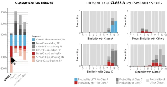
Finally, 2 potential users requested the visualization of errors over similarity scores, prior to applying logistic regression. We thus devised the visualization in Fig. 10
where users can select a class to investigate, and visualize error distributions over (1) the similarity scores of the class of interest, (2) the similarity scores of the most confused classes, and (3) compare these with the overall distribution for other classes. Such visualizations can support users in acquiring a better understanding of the uncertainty and of the underlying computational processes. It can also help technology providers improve their algorithm (e.g., modi-fying the computation of similarity scores by weighting the underlying features used to recognize objects), or detect the need for collecting additional groundtruth items (e.g., classes implying high numbers of errors for high similarity scores, which may indicate that the groundtruth sets are not discriminative enough). Other use cases or user groups may require different designs visualizing other types of distribu-tion (e.g., over low-level item features).
Future work will investigate visualizations for exploring error distribution over similarity scores or other features. Future work will also empirically evaluate our design. We will compare user behaviour with our visualization, the usual ROC and Precision/Recall curves, or with confu-sion matrix enhanced with overlaid heatmap (coloring the
cells according to error magnitudes). We will investigate user effectiveness and efficiency in understanding potential biases in end-results, as well as user trust in the machine learning system. Experiments will include both machine learning experts and non-experts.
6 Conclusion
We specified and evaluated a novel method for estimating the biases of supervised machine learning classification. It significantly improves counting results by fitting logistic regression functions on similarity scores.1 We provide
tem-plates for user-friendly visualization of the end-results’ uncertainty, and explanations of the counting method. Our work addresses user needs for visualizing biases due to interclass confusions. It is robust to end-usage issues with groundtruth test sets under- or over-representing relative classes’ abundance, and distribution of similarity scores
amongst actual items to classify. It is widely applicable to automatic counting tasks, and provides an accessible uncer-tainty evaluation.
References
1. Alsallakh, B., Hanbury, A., Hauser, H., Miksch, S., Rauber, A.: Visual methods for analyzing probabilistic classification data. Vis. Comp. Graph. IEEE Trans. 20(12), 1703–1712 (2014) 2. Beauxis-Aussalet, E., Hardman, L., van Ossenbruggen, J.:
Deliv-erable D2.1 of the Fish4Knowledge Project-User information needs. Tech. rep. http://groups.inf.ed.ac.uk/f4k/DELIVERA-BLES/Del21.pdf
1 A measure of features’ similarity comparing an item to classify and
a class model (Sect. 3.1). Fig. 10 Visualization of error
distributions over similarity scores
Similarity with Class A
0 1 Probabilit y 1 2 3 4 5 6 7 8 9 10 0
Probability of TP for Class A Probability of FP for Class A
Probability of Class C Probability of other Classes Probability of Class F
PROBABILITY OF CLASS A OVER SIMILARITY SCORES
CLASSIFICATION ERRORS Class C Class A Class F Average O ther 100% 200% 300% -200% -100%
Similarity with Class C 0
1
1 2 3 4 5 6 7 8 9 10 0
Probability
Mean Similarity with Others
0 1 1 2 3 4 5 6 7 8 9 10 0 Probabilit y
Similarity with Class F
0 1
1 2 3 4 5 6 7 8 9 10 0
Probability
Main Class drawing FN Second Class drawing FN Other Class drawing FN Second Class adding FP
Legend:
Main Class adding FP Other Class adding FP
3. Beauxis-Aussalet, E., Arslanova, E., Hardman, L., van Ossen-bruggen, J.: A case study of trust issues in scientific video col-lections. In: Proceedings of the 2nd ACM international workshop on Multimedia analysis for ecological data. ACM (2013) 4. Beauxis-Aussalet, E., Arslanova, E., Hardman, L., van
Ossen-bruggen, J.: A video processing and data retrieval framework for fish population monitoring. In: Proceedings of the 2nd ACM international workshop on Multimedia analysis for ecological data. ACM (2013)
5. Beauxis-Aussalet, E., Hardman, L.: Visualization of confusion matrix for non-expert users. In: Poster at the IEEE Conference on Visualization—IEEE VIS (2014)
6. Bliss, C.: The method of probits. Science 79(2037), 38–39 (1934)
7. Chan, A.B., Liang, Z.S., Vasconcelos, N.: Privacy preserving crowd monitoring: counting people without people models or tracking. In: Conference on computer vision and pattern recogni-tion—CVPR, pp. 1–7. IEEE (2008)
8. Chen, C.: Top 10 unsolved information visualization problems. Computer Graphics and Applications, IEEE 25(4), 12–16 (2005) 9. Correa, C.D., Chan, Y.H., Ma, K.L.: A framework for
uncer-tainty-aware visual analytics. In: IEEE Symposium on visual analytics science and technology—VAST, pp. 51–58 (2009) 10. Gibson, R., Barnes, M., Atkinson, R.: Practical measures of
marine biodiversity based on relatedness of species. Oceanogr. Mar. Biol. Ann. Rev. 39, 207–231 (2001)
11. Hay, A.: The derivation of global estimates from a confusion matrix. Int. J. Remote Sens. 9(8), 1395–1398 (1988)
12. Hetrick, N.J., Simms, K.M., Plumb, M.P., Larson, J.P.: Feasibil-ity of using video technology to estimate salmon escapement in the Ongivinuk River, a clear-water tributary of the Togiak River. US Fish and Wildlife Service, King Salmon Fish and Wildlife Field Office (2004)
13. Houben, S., Stallkamp, J., Salmen, J., Schlipsing, M., Igel, C.: Detection of traffic signs in real-world imagvucetices: the ger-man traffic sign detection benchmark. In: International Joint Conference on Neural Networks. No. 1288 (2013)
14. Huang, P.X., Boom, B.J., Fisher, R.B.: GMM improves the reject option in hierarchical classification for fish recognition. In: IEEE Winter Conference on applications of computer vision—WACV, pp. 371–376 (2014)
15. Irvine, J., Ward, B., Teti, P., Cousens, N.: Evaluation of a method to count and measure live salmonids in the field with a video camera and computer. North Am. J. Fish. Manag. 11(1), 20–26 (1991)
16. Johnson, C.: Top scientific visualization research problems. Comput. Graph. Appl. IEEE 24(4), 13–17 (2004)
17. Jupp, D.L.B.: The stability of global estimates from confusion matrices. Int. J. Remote Sens. 10(9), 1563–1569 (1989)
18. Lehmussola, A., Ruusuvuori, P., Selinummi, J., Huttunen, H., Yli-Harja, O.: Computational framework for simulating fluores-cence microscope images with cell populations. Med. Imaging IEEE Trans 26(7), 1010–1016 (2007)
19. Lempitsky, V.S., Zisserman, A.: Learning to count objects in images. In: NIPS. vol. 1, p. 2 (2010)
20. Lip, C., Ramli, D.: Comparative study on feature, score and deci-sion level fudeci-sion schemes for robust multibiometric systems. In: Sambath, S., Zhu, E. (eds.) Frontiers in computer education, advances in intelligent and soft computing, vol. 133, pp. 941– 948. Springer, Berlin, Heidelberg (2012)
21. McCullagh, P., Nelder, J.A.: Generalized linear models, vol. 2. Chapman and Hall, London (1989)
22. Platt, J.C.: Probabilistic outputs for support vector machines and comparisons to regularized likelihood methods. In: Advances in large margin classifiers. Citeseer (1999)
23. Saerens, M., Latinne, P., Decaestecker, C.: Adjusting the outputs of a classifier to new a priori probabilities: a simple procedure. Neural Comput. 14(1), 21–41 (2002)
24. Tulp, I., Bolle, L.J., Rijnsdorp, A.D.: Signals from the shallows: in search of common patterns in long-term trends in dutch estua-rine and coastal fish. J. Sea Res. 60(1), 54–73 (2008)
25. Visser, H.: Estimation and detection of flexible trends. Atmos. Environ. 38(25), 4135–4145 (2004)
26. Vucetic, S., Obradovic, Z.: Classification on data with biased class distribution. In: Proceedings of the 12th European confer-ence on machine learning. pp. 527–538. Springer (2001) 27. Ware, C.: Information visualization: perception for design.
Else-vier (2013)
28. Watson, D.L., Harvey, E.S., Anderson, M.J., Kendrick, G.A.: A comparison of temperate reef fish assemblages recorded by three underwater stereo-video techniques. Mar. Biol. 148(2), 415–425 (2005)
29. Willis, T.J., Babcock, R.C.: A baited underwater video system for the determination of relative density of carnivorous reef fish. Mar. Freshw. Res. 51(8), 755–763 (2000)
30. Yoshida, T., Akagi, K., Toda, T., Kushairi, M., Kee, A., Othman, B.: Evaluation of fish behaviour and aggregation by underwater videography in an artificial reef in tioman island, malaysia. Sains Malays. 39(3), 395–403 (2010)