Applied Machine Learning for Classification of Musculoskeletal Inference using Neural Networks and Component Analysis

(1)

University of Denver University of Denver

Digital Commons @ DU

Electronic Theses and Dissertations Graduate Studies

1-1-2019

Applied Machine Learning for Classification of Musculoskeletal

Inference using Neural Networks and Component Analysis

Shaswat Sharma

University of Denver

Follow this and additional works at: https://digitalcommons.du.edu/etd

Part of the Artificial Intelligence and Robotics Commons

Recommended Citation Recommended Citation

Sharma, Shaswat, "Applied Machine Learning for Classification of Musculoskeletal Inference using Neural Networks and Component Analysis" (2019). Electronic Theses and Dissertations. 1619.

https://digitalcommons.du.edu/etd/1619

This Thesis is brought to you for free and open access by the Graduate Studies at Digital Commons @ DU. It has been accepted for inclusion in Electronic Theses and Dissertations by an authorized administrator of Digital

(2)

Applied Machine Learning for

Classification of Musculoskeletal Inference using Neural Networks and Component Analysis

A Thesis Presented to the Faculty of the Daniel Felix Ritchie School of Engineering and Computer Science

University of Denver

In Partial Fulfillment

of the Requirements for the Degree Master of Science

by

Shaswat Sharma June 2019

(3)

(4)

Author: Shaswat Sharma

Title: Applied Machine Learning for Classification of Musculoskeletal Inference using Neural Networks and Component Analysis

Advisor: Matthew Rutherford Degree Date: June 2019

Abstract

Artificial Intelligence (AI) is acquiring more recognition than ever by researchers and machine learning practitioners. AI has found significance in many applications like biomedical research for cancer diagnosis using image analysis, pharmaceutical research, and, diagnosis and prognosis of diseases based on knowledge about patients’ previous conditions. Due to the increased computational power of modern computers implementing AI, there has been an increase in the feasibility of performing more complex research.

Within the field of orthopedic biomechanics, this research considers complex time-series dataset of the “sit-to-stand” motion of 48 Total Hip Arthroplasty (THA) pa-tients that was collected by the Human Dynamics Laboratory at the University of Denver. The research focuses on predicting the motion quality of the THA patients by analyzing the loads acting on muscles and joints during one motion cycle. We have classified the motion quality into two classes: “Fair” and “Poor”, based on muscle forces, and have predicted the motion quality using joint angles.

We address different types of Machine Learning techniques: Artificial Neural Net-works (LSTM - long short-term memory, CNN - convolutional neural network, and merged CNN-LSTM) and data science approach (principal component analysis and parallel factor analysis), that utilize remodeled datasets: heatmaps and 3-dimensional vectors. These techniques have been demonstrated efficient for the classification and prediction of the motion quality.

The research proposes time-based optimization by predicting the motion quality at an initial stage of musculoskeletal model simulation, thereby, saving time and efforts required to perform multiple model simulations to generate a complete musculoskele-tal modeling dataset. The research has provided efficient techniques for modeling neu-ral networks and predicting post-operative musculoskeletal inference. We observed

(5)

the accuracy of 83.33% for the prediction of the motion quality under the merged LSTM and CNN network, and autoencoder followed by feedforward neural network. The research work not only helps in realizing AI as an important tool for biomedical research but also introduces various techniques that can be utilized and incorporated by engineers and AI practitioners while working on a multi-variate time-series wide shaped data set with high variance.

(6)

Acknowledgements

It gives me great pleasure to thank all the important people who have helped me during the thesis, without whom, thesis completion would have been next to impossible.

My heartiest thanks to my parents, Jagdish and Jyotsna, and my brother, Ateet, for their endless love and faith in me that always inspired me to work harder.

I want to express my sincere gratitude towards my research advisor, Dr. Matthew Rutherford, who has been very generous in providing me the knowledge and his time for troubleshooting and brainstorming. While working on the research, he scheduled numerous meetings with me and always guided me in the right direction; applying that in the research work produced tremendously improved and accurate results. I could not think of any better mentor than Dr. Matt.

I would also like to thank my defense committee members, Rinku Dewri and Laleh Mehran, for reviewing my thesis and for being part of my oral defense committee. Their valuable insights have helped me incredibly in delivering the work.

The University of Denver is a wonderful school that has always maintained an accomplishing sentiment in my heart. I feel proud to be a graduate student at the school where I have learned a great deal of science.

Last but not the least, I would like to thank my friends and colleagues for their continuous encouragement.

(7)

List of Figures

2.1 Total Hip Arthroplasty : Before surgery1 _{. . . .} ₈

2.2 Total Hip Arthroplasty : After surgery1 _{. . . .} ₈

2.3 Types of motion [23] . . . 11

2.4 Motion capture system2 _{. . . .} ₁₁

2.5 Before normalization . . . 14

2.6 After mean centering . . . 14

2.7 After relative variation scaling . . . 15

2.8 PCA, mean squared error minimization on two components . . . 18

2.9 Logistic regression curve [23] . . . 24

2.10 Schematic of biological neuron [38] . . . 25

2.11 Schematic of ANN . . . 26

2.12 Schematic of artificial neuron [37] . . . 26

2.13 Recurrent neural network . . . 30

2.14 Long Short-Term Memory . . . 30

2.15 LeNet5 [24] . . . 31

2.16 AlexNet [25] . . . 32

2.17 Undercomplete autoencoder . . . 34

2.18 Autoencoder contrast with PCA 2.5.1 . . . 34

2.19 ANN approach by Danaee et. al for cancer detection [42] . . . 36

2.20 Logistic sigmoid function . . . 38

2.21 Hyperbolic tangent function . . . 39

2.22 Rectified linear unit . . . 40

3.1 Sit To Stand Motion Cycle . . . 43

3.2 Three stages of OpenSim motion analysis [40] . . . 44

3.3 Hip Musculature 1 3 _{. . . .} ₄₄

3.4 Quadriceps femoris muscles 3 _{. . . .} ₄₅

3.5 Supervised learning using the dataset . . . 48

3.6 Original input sequence for patient 1 . . . 50

3.7 Mean centered input sequence for patient 1 . . . 51

3.8 Relative variation scaled sequence for patient 1 . . . 51

3.9 Patient 1 profile with selected features . . . 53

(11)

3.11 Patient 46 profile with selected features . . . 54

3.12 Contrasting forces on left knee joint of patient 32 with other patients 55 4.1 Research and Analysis flow chart, Phase 1 . . . 58

4.2 Vastus Medialis Load Delta, Patient 29 . . . 60

4.3 Dominant section occurrences for all the patients using the Feature Set 1 62 4.4 (a) Feature delta contrast for patient 3 using Feature Set 1 . . . 63

4.5 (b) Feature delta contrast for patient 3 using Feature Set 1 . . . 64

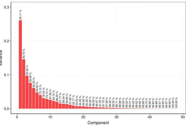
4.6 Variance in the components generated by the PCA on the mean cen-tered inverse kinematic features . . . 67

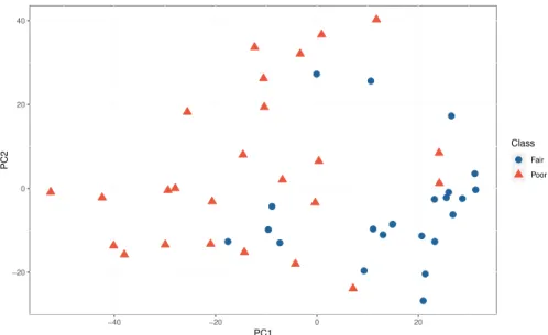
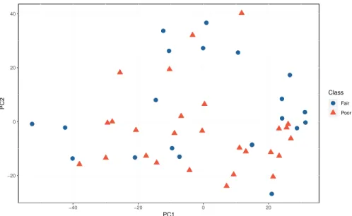
4.7 Clustering of the patients using motion quality categories using the Feature Set 1, and components generated using all the mean centered inverse kinematics features . . . 68

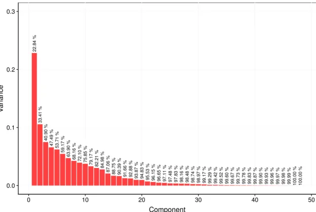
4.8 Variance in the components generated by the PCA on the relative variation scaled inverse kinematic features . . . 69

4.9 Clustering of the patients using motion quality categories using the Feature Set 1, and components generated using all the relative variation scaled inverse kinematics features . . . 70

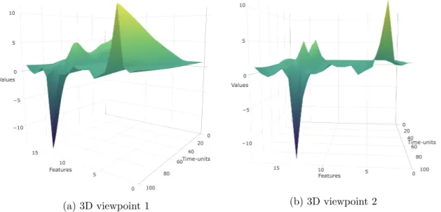
4.10 3D model of original inverse kinematic features for patient 1 . . . 71

4.11 3D visualization of mean centered inverse kinematic features for patient 1 72 4.12 Clustering of the patients using motion quality categories using the Feature Set 1, and PARAFAC components generated using all the mean centered inverse kinematics features . . . 72

4.13 3D model of relative variation scaled inverse kinematic features for patient 1 . . . 73

4.14 Clustering of the patients using motion quality categories using the Feature Set 1, and PARAFAC components generated using all the relative variation scaled inverse kinematics features . . . 74

4.15 PC1 loadings for mean centered inverse kinematics features . . . 79

4.16 Clustering form by PCA using mean centered top 6 inverse kinematics features and motion quality quantified using Feature Set 3 . . . 80

5.1 Bridging the gap between inverse kinematics and motion quality . . . 81

5.2 Research and Analysis, Phase 2, work flow . . . 82

5.3 Undercomplete autoencoder used for dimensionality and noise reduc-tion on inverse kinematics dataset . . . 86

5.4 Mean centered feature set 3 . . . 87

5.5 Feature set 3, Remodeled, Range 0 to 1 . . . 87

5.6 Reconstructed input dataset using the autoencoder . . . 88

5.7 Output of the encoding layer for patient 1 . . . 89

5.8 Feedforward followed by autoencoder, iteration 1, 64.58% accuracy . . 90

(12)

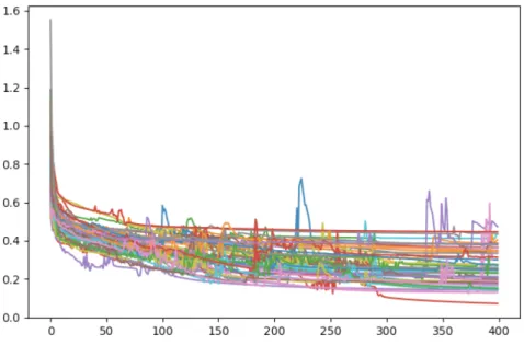
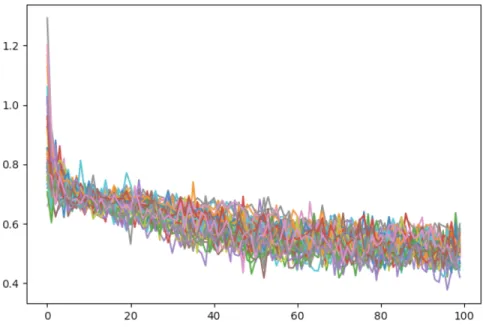
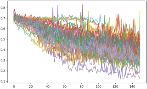
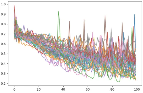
5.12 Feedforward followed by Autoencoder, final iteration, 83.33% accuracy 93 5.13 Loss curve of the 48 cross-validation training steps using network in the final iteration . . . 93

5.14 Feedforward, iteration 1, 75.0% accuracy . . . 95

5.15 Feedforward, iteration 2, 75% accuracy . . . 96

5.16 Feedforward, iteration 3, 77% accuracy . . . 97

5.17 Feedforward, final iteration, 81.25 % accuracy . . . 98

5.18 Loss curve of the 48 cross-validation training steps using the feedfor-ward network in the final iteration . . . 99

5.19 Convolutional neural network, iteration 1, accuracy 58.33% . . . 99

5.22 Convolutional Neural Network, final iteration, accuracy 79.16% . . . 101

5.23 Loss curve of the 48 cross-validation training steps using the CNN network in the final iteration . . . 102

5.24 LSTM, iteration 1, accuracy 60.41% . . . 103

5.28 Loss curve of the 48 cross-validation training steps using the LSTM network in the final iteration . . . 107

5.29 Merged CNN LSTM, accuracy 83.33% . . . 108

5.30 Loss curve of the 48 cross-validation training steps using the merged CNN LSTM network . . . 109

1 Bias-variance dilemma . . . 117

2 Bias-variance error . . . 118

3 Clustering by PCA using inverse kinematic mean centered features and motion quality quantified using feature set 2 . . . 129

(13)

10 Clustering by PCA using inverse kinematic mean centered features and motion quality quantified using feature set 9 . . . 132 11 Clustering by PCA using inverse kinematic relative variation scaled

features and motion quality quantified using feature set 2 . . . 133 12 Clustering by PCA using inverse kinematic relative variation scaled

features and motion quality quantified using feature set 9 . . . 136 19 Clustering by PARAFAC using inverse kinematic mean centered

fea-tures and motion quality quantified using feature set 2 . . . 137 20 Clustering by PARAFAC using inverse kinematic mean centered

fea-tures and motion quality quantified using feature set 9 . . . 140 27 Clustering by PARAFAC using inverse kinematic relative variation

scaled features and motion quality quantified using feature set 2 . . . 141 28 Clustering by PARAFAC using inverse kinematic relative variation

(14)

31 Clustering by PARAFAC using inverse kinematic relative variation scaled features and motion quality quantified using feature set 6 . . . 143 32 Clustering by PARAFAC using inverse kinematic relative variation

(15)

Chapter 1

Introduction

Machine Learning (ML), a subfield of Artificial Intelligence (AI), is the field of computer science that attempts to mimic the cognitive functions like learning and problem solving that a human brain does. With the help of AI techniques, machines have been successful in demonstrating intelligent behavior imitating human intelli-gence. Based on past experience, the machines can make decisions on a new set of information that represents the analytical ability to respond to a new environment. Some of the practical applications of AI are natural language processing like Siri, Alexa and Cortana, image analysis for object recognition, medical diagnosis, time-series predictions for stock markets, and so on. Recently, AI is powered by Artificial Neural Networks (ANN) to analyze big data and enable such applications.

ANN is a self-learning programming framework loosely inspired by the biological organization of animal brains. The design of ANN is such that they are meant to replicate the way humans learn. ANN aid the computing systems to assimilate and learn using observational data and ML algorithms. The ANN model performs tasks by “learning” from a set of input-output examples, rather than being programmed with a set of rules. The accuracy of a neural network depends on multiple factors, one of which is the size of the dataset (number of input-output examples) available as input to the network. A larger dataset gives more information on the input test cases, and hence, it enables robust learning.

(16)

Due to the increasing availability of data, AI has also flourished in the field of med-ical science by helping doctors and clinicians improve different aspects of health care like prevention of diseases, providing effective treatments to patients, disease progno-sis, pre-operative and post-operative care of surgical procedures and pharmaceutical drugs, among others. The availability of a patient’s medical history and previous medical cases allows systems to extract knowledge and analyze future instances. In the biomedical orthopedic industry, scientists are using the latest technologies exten-sively to improve orthopedics with robot-assisted surgery, improved designs of pros-thetic implants, shoe designing for different purposes for the best comfort of users, and many more.

Human dynamics, a branch of orthopedic biomechanics, focuses on studying the human musculoskeletal system to improve clinical diagnosis and treatment through biomechanical measurement and analysis. A human musculoskeletal system encom-passes the organ system that gives humans the ability to perform movements using the muscular and skeletal systems. It consists of joints, bones, muscles, ligaments, cartilage, and various other connective tissues. The availability of software for biome-chanical modeling, simulation, and analysis has helped in improving the study of human dynamics with efficient data collection of the human body movements [3].

Human motion analysis of a subject’s gait, sit-to-stand, and step-down movements has been useful in the field of sports, kinesiology, physical therapy, and surgical anal-ysis. Surgeries like knee arthroplasty, hip joint replacement, laminectomy, and spinal fusion are the consequences of reduced mobility of human body movements and are common in United States [1]. Motion analysis has enabled clinicians to assess and treat patients with deficiencies in body movement. Motion discrepancy in the mus-culoskeletal system can be observed at a fine level of detail with the help of advanced machinery that captures the motion of patients, which is further analyzed by simu-lating a virtual musculoskeletal model. Quantifying the human motion into joint and muscle forces helps in assessing post-operative impacts on the patients.

Total Hip Arthroplasty (THA) or hip replacement surgery is a common surgical procedure used for the treatment of joint failure caused by osteoarthritis. The hip joint is the amalgamation of the femoral head (the highest part of the thigh bone) and acetabulum (cavity where femoral head and pelvis meet). THA involves the

(17)

substitu-tion of both femoral head and acetabulum with prosthetic implants. The alignment of the three synthetic components significantly influences post-surgical motion qual-ity [4]. To study the component alignment for the hip replacement surgery, scientists and researchers in the Human Dynamics Laboratory (HDL) at the University of Den-ver have collected the musculoskeletal data of THA patients using equipment like force platforms, electronic markers, motion capture systems, and OpenSim software. We use the same musculoskeletal dataset to assess the motion quality of THA patients with ML.

1.1

Problem Statement

This research addresses the application of machine learning and data science in the field of orthopedic biomechanics by utilizing various ANN architectures and applying data science approaches. The work comprises of the quantitative analysis of the THA patients’ body movements and assessment of their motion quality, based on data science and ML models. The resulting motion quality metric can help modify the component alignment to improve the results of a surgical procedure and enable improved prosthetic implantation.

We have used the musculoskeletal data quantified by the HDL for the post-surgical “sit-to-stand” motion of 48 THA patients. The dataset contains variables corre-sponding to skeletal joints (pelvis, hip, knee, ankle and lumbar) and muscles (biceps femoris, semimembranosus, semitendinosus, gluteus, rectus, vastus, gastrocnemius, and soleus) of the lower extremity. Thus, the attributes of the patient dataset en-tirely correspond to the bio-medical field and are more understandable to the doctors and the clinicians. We, being the researchers in the field of Computer Science, at-tempt to comprehend the data and make inferences using ML techniques. The dataset has 48 records each with 7502 columns, with 75 time-series features, each having 100 time units. However, standard ML algorithms prefer many thousands of records, and to account for that, we have analyzed the data efficiently by applying various ANN models.

The motion quality of THA patients is quantified using data science approaches like principal component analysis and parallel factor analysis, and it is classified into two classes: “Fair” and “Poor”. The research proposes to predict the quantified motion

(18)

quality from the first stage of data simulation, inverse kinematics, instead of simulat-ing the variables of the other two consecutive stages - inverse dynamics and muscle force prediction. The motion quality is thus, predicted from time-series variables of inverse kinematics using ANN models like feedforward, CNN (Convolutional neural network), LSTM (Long short-term memory), and auto-encoders.

1.2

Summary of Contributions

The research work has addressed various methods, techniques, and approaches, for engineers and researchers engaged in the field of machine learning. The contributions can be summarized as follows:

• Motion quality quantification: This work discusses how we use the THA patients’ dataset and remodel it by applying various techniques to quantify the motion quality. As there is no standard way to assess the motion quality from the available muscle force attributes of the dataset, we have devised a method for relative analysis between the patients that can help us quantify the motion quality.

• Motion quality discovery: Using component analysis techniques, we dis-covered the existence of quantified motion quality in the joint angle dataset of the lower extremity. Further, we used the results of the analysis for inverse kinematics feature selection and to improve the motion quality quantification.

• Shortened process to predict motion quality: This research describes the application of various ANN models to predict the quantified motion quality from the time-series variables of inverse kinematics (the first stage of musculoskeletal data simulation). It eliminates the need to calculate the variables of inverse dynamics and muscle force prediction.

• Wide-shaped and high variance data utilization: The dataset used is wide-shaped and has high variance; such a dataset is considered unreliable in machine learning. This work demonstrates efficient data science techniques and neural network models for such an input dataset.

• Remodeled time-series data analysis: We remodeled the time-series dataset into 2-dimensional and 3-dimensional vectors and used them in two different component analysis techniques for the discovery of motion quality in the joint

(19)

angle dataset. Also, we used the remodeled datasets along with heatmaps to train the neural network models to learn and classify the motion quality of each patient efficiently.

• Motion quality prediction: We have predicted the classified motion quality via muscle forces, using the joint angles by ANN, with an accuracy of 83.33%.

1.3

Organization of Thesis

The thesis work is structured around the following chapters:

• Related Work and Background: This chapter explores the previous research work and relevant contributions made in the field of ANN and musculoskeletal modeling. It also describes various ANN models and data science approaches, and concepts related to them, that are used in this research.

• System Description: This chapter encompasses the data collection process and data normalization techniques. It has a description of the data simulation stages for musculoskeletal modeling viz inverse kinematics, inverse dynamics, and muscle force predictions. It also focuses on narrowing the body features that are most relevant to the motion quality analysis. The chapter also presents the relative motion analysis of one patient against other patients.

• Research and Analysis: This chapter constitutes the primary research work and analysis that builds this thesis. It consists of the following:

– Motion quality analysis, quantification, classification, and verification.

– Application of the component analysis to get the most concentrated and relevant information from the wide-shaped dataset, achieved by data re-modeling.

– Motion quality evolution by selection of relevant features for prediction and classification.

– Assessment of conventional regression methods over the dataset in appli-cation.

– Exploration and application of ANN models to perform data compression and prediction of motion quality, using different remodeled datasets like heatmaps, time-series, 2-dimensional and 3-dimensional vectors.

(20)

– Development of good performance networks to achieve high accuracy for motion quality prediction.

• Conclusions and Future Work: This chapter summarizes the contributions of the research work and talks about the ways to explore this work further.

(21)

Chapter 2

Related Work and Background

2.1

Total Hip Arthroplasty

The hip joint is analogous to a ball-socket joint where the spherical ball lying in the socket enables the rotation and multi-directional movement of the coupling. In a hip joint, the femoral head (top of the thigh bone) acts as the ball, and the acetabulum (cavity where femoral head and pelvis meets) serves as the socket, allowing the smooth movement of the hip joint [20]. Figure 2.1 depicts the hip joint and its components.

Hip joint deterioration can be caused by osteoarthritis A.2.1, inflammatory arthritis A.2.2, infancy hip disorders, trauma and osteonecrosis A.2.3. Non-surgical treatments like physical therapy, weight loss, using a walker, medications or steroid injections are recommended to treat a bad hip before resorting to the surgical procedure of Total Hip Arthroplasty (THA).

In the procedure of THA, prosthetic implants made from metal or plastic replace the deteriorated hip joint. The femoral head and the acetabulum are replaced with a prosthetic femoral component and an acetabular cup respectively. The femoral component is made of the femoral head and femoral stem. In the surgical procedure, the acetabular cup is fitted with the femoral component with a plastic liner to enable a smooth, realistic movement of the prosthetic hip joint. Figure 2.2 depicts the post-surgical view of the hip joint along with the prosthetic components.

Hip replacement surgeries have been one of the most common orthopedic surgical operations in the United States with a reliable success rate [16]. As THA involves

(22)

Figure 2.1: Total Hip Arthroplasty : Before surgery 1

Figure 2.2: Total Hip Arthroplasty : After surgery 1

the replacement of the hip with prosthetic implantation, the component alignment significantly impacts the post-surgical quality of motion. Component mishaps like impingement, dislocation, component degradation, and edge loading, affect the com-ponent alignment which consecutively incurs changes in femoral anteversion and in-creases hip joint contact forces [17]. Such issues lead to a revision THA which is undesirable. Inferring knowledge about the post-surgical quality of motion can be beneficial to reduce the number of revision THA, and also perform the first THA in other patients with more precision.

(23)

Machine learning techniques have been used for the optimization of joint replace-ments. Cilla et al. [41] used the following two techniques to solve the prosthetic implant optimization problem:

• Artificial Neural Networks (ANN)

• Support Vector Machines (SVM)

They investigated the geometry of a commercial short stem hip prosthesis using the following implant geometrical parameters:

• Total stem length

• Thickness in the lateral and medial stem sides

• Distance between the central stem surface and the implant neck

The machine learning techniques they used on these parameters showed that opti-mization in the prosthetic implant is significantly dependent on the decrease in stem length and reduction in the length of the surface in contact with the bone.

2.2

Motion Capture

The process of capturing the human body movements into a digital environment, using motion capture equipment like high-resolution cameras and electronic markers (sensors) is known as motion capture. The process of motion capture involves record-ing the motion usrecord-ing marker placements, transformrecord-ing the data into digital form and integrating the data using analytical software.

There are three types of motion capture systems:

1. Magnetic: Sensor-based system where sensors are placed on different body parts. The sensors are wired to a computer that fetch the data correspond-ing to marker coordinates.

2. Mechanical: Motion is captured using a skeleton-shaped body suit. Each joint is attached with a sensor that gives the relative coordinates of the sensors. 3. Optical: Motion is captured digitally using reflective and pulse LEDs. Multiple

cameras are placed at different angles in the environment to create a sense of three dimensions. The sensors are placed on the body, and their positions are mapped into a 3D environment using a computer software.

(24)

Researchers working with the Human Dynamics Lab at the University of Denver have used an optoelectronic sensor-based motion capture system to record the “sit-to-stand” motion of THA patients. The sensors attached to the body are called markers. Figure 2.4 gives an overview of the working of the marker-based motion capture system.

Vicon motion capture [13] is one of the most precise marker based optoelectronic motion capture system with a system error of less than 2mm (between actual marker position and software generated marker coordinates) [19]. During the process of mo-tion capture, each body movement is captured across multiple time frames (many times per second) by the electronic markers placed at different places on the body. The markers, acting as sensors, broadcast the captured data to the motion capture software which then generates a 3-dimensional simulated skeleton model correspond-ing to the body motion.

2.3

Musculoskeletal Modeling

The musculoskeletal models are computational models simulating the human skele-tal system that are composed of rigid bodies replicating the bones bridged by me-chanical joints. Actuators represent the muscles to provide joint torques mirroring the body movement. Figure 2.3 depicts a simulated musculoskeletal model for three types of motion: gait, step down and sit-to-stand.

External forces on the human body have an impact on the internal muscle loads. To observe the relation between the human body movements and loads on the muscles during the movements, motion analysis is performed using musculoskeletal models. With the advancement in technology, the external forces are quantifiable with the force platforms (instruments to measure the ground reaction forces generated by the motion of the body) but quantifying internal muscle loads, and joint reaction forces are not feasible due to its invasiveness. Musculoskeletal models have been introduced to reach an almost accurate estimation of the parameters.

Musculoskeletal Simulation

The marker-based motion capture system records the human motion and trans-forms it into a musculoskeletal model with the motion capture software. The

(25)

ex-Figure 2.3: Types of motion [23]

Figure 2.4: Motion capture system 2

perimental techniques performed using the marker placement lack to bridge the gap between the muscular dynamics and human motion, and hence, the human body motion analysis is performed by mirroring the recorded human motion into a mus-culoskeletal simulation using tools like OpenSim [11], which is then segmented into three consecutive stages for motion analysis:

(26)

• Inverse Kinematics

• Inverse Dynamics

• Muscle Force Prediction

Inverse Kinematics

In inverse kinematics modeling, the best fit model is generated to match the ex-perimental markers with the model markers for the simulated motion by minimizing the sum of weighted squared errors of the markers and coordinates throughout the motion cycle. The Inverse Kinematics (IK) toolkit, available with the OpenSim soft-ware, enables the implementation of the inverse kinematics stage. The output of this simulation stage contains generalized coordinate trajectories in the form of joint angles and translations of the motion.

Inverse Dynamics

In inverse dynamics, forces and torques, that produce the body movement, are measured at each joint, based on the kinematics information available for the motion of the model. The inverse dynamics analysis is performed using the Inverse Dynamics (ID) toolkit of OpenSim. The output of this simulation stage contains time-based joint forces and torques that produces the accelerations based on measured exper-imental movement and external forces acting on the model. Overall, the inverse dynamics stage focuses on solving the equation of motions for the unknown general-ized forces by using the known motion of the model, where the positions, velocities, and accelerations define the motion of the model.

Muscle Force Prediction

Using the outputs of the inverse kinematics stage and the inverse dynamics stage, along with a Hill-type muscle model, the muscle forces are predicted. A Hill-type muscle model corresponds to the Hill’s equations for the tetanic muscle contraction in investigations over cadavers [22].

To perform post-surgical motion analysis of the THA patients, the quality of the motion is measured based on the forces acting on the muscles during the body move-ment. Due to the infeasibility of the process to measure such forces, musculoskeletal

(27)

simulation is used to estimate the forces acting on the muscles during the human body movement.

2.4

Statistics : Prerequisites

2.4.1

Mean Centering

A subject dataset in an application can consist of multiple features having different measuring units and magnitude ranges. The difference in magnitude ranges will affect the significance of the features when analyzed all together. To overcome this issue, we perform mean centering on the data so that the values of features bounds around the mean zero. This process introduces a new dataset with a comparable range of magnitudes of the features that enhance the overall significance of the data.

Algorithm 1 is used to perform mean centering on every data point in a time series by subtracted by the mean of the complete series.

Algorithm 1 Mean Centering

Input: F1. . . Fm f or P1. . . Pn

Output: Zero M ean Centered Series

1: function MeanCentering(F) 2: for p←1 to n do 3: mean[p] = Pm to=1F[p,to] m 4: for t←1 to m do 5: F[p, t] =F[p, t]−mean[p] 6: end for 7: end for 8: return F 9: end function

Figure 2.5 represents three time series with different range of magnitudes. After performing mean centering, the series transforms to a comparable magnitude range as shown in Figure 2.6.

2.4.2

Relative Variation Scaling

Relative Variation Scaling, algorithm 2, is a technique to normalize the data by calculating the factor of change in a time series with respect to the initial data point

(28)

0 100 200 300 400 0 100 200 300

Time Series Features

V

alues

Figure 2.5: Before normalization

−20 0 20

0 100 200 300

V

alues

Figure 2.6: After mean centering

in the series. Applying this technique, a time series transforms to originate from value 1 and the overall magnitude range of the series gets minimized by the factor of the initial data point of the original series. By concatenating multiple time series, variability in each series can be compared.

If the time series starts with a negative number, before performing the normal-ization, the time series should be transformed so that every data point in the series becomes positive. This preserves the relative variation in the series, viz growth or descent.

(29)

Algorithm 2 Relative Variation Scaling

Input: F1. . . Fm f or P1. . . Pn

Output: Relative V ariation Scaled Series

1: function Relative Variation Scaling(F) 2: for p←1 to n do 3: for t←1 to m do 4: F[p, t] =F[p, t]/F[p,0] 5: end for 6: end for 7: return F 8: end function

Taking the same example in Figure 2.5, after relative variation scaling, the three time series will be transformed as depicted in Figure 2.7. The overall range of con-catenated series will be between the highest growth factor and the smallest descent factor. 0.9 1.0 1.1 1.2 1.3 0 100 200 300

V

alues

Figure 2.7: After relative variation scaling

2.5

Dimensionality Reduction

When working with multivariate time series data, the count of columns exceeds by the factor of time series intervals and increases the complexity of data by adding more dimensions to statistical regression models. To simplify the regression methods and

(30)

condense the information included in the original data to a more comprehensible form, dimensionality reduction [30] plays an important role. Principal Component Analysis (PCA) and Parallel Factor Analysis (PARAFAC) are the techniques we explore to perform dimensionality reduction. Both the methods work similarly by projecting the original data points to a set of orthogonal vectors called principal components. PCA is an efficient technique for a dataset with a shape like a 2-dimensional matrix, whereas, PARAFAC is an advanced version of PCA which applies to a more complex, multi-way dataset that has more than two dimensions. Both the techniques are used to perform dimensionality reduction on the musculoskeletal time series data. The compressed information is used to visualize the relationship between musculoskeletal inferences and the input time series data.

2.5.1

Principal Component Analysis (PCA)

Pearson coined the idea of PCA in 1901 [31]. It was also independently developed by Hotelling in 1936 [32, 33]. Phinyomark et al. provided a review of how the PCA techniques were used for gait analysis for various research questions [44] as follows:

• Differentiating between healthy and unhealthy female runners

• Predicting the response to exercise treatment for patients with patellofemoral pain and knee osteoarthritis

• Analyzing body movement differences occurring due to wearing shoes with dif-ferent midsoles

Kirkwood et al. applied PCA on the gait kinematics data of elderly women suffering from knee osteoarthritis. They found the PCA technique to be effective to analyze the kinematic gait form during the gait cycle. They were able to find the most significant component which acted as the discriminatory factor between the group of females with and without osteoarthritis. This component could be used for physical therapy evaluation and treatment of the women with osteoarthritis [45].

PCA is a linear technique for dimensionality reduction of a large number of data points correlated with each other that maps the original data points to a lower dimen-sional linear vector called Principal Component (PC), such that the variance of the data points in the lower dimension maximizes. The variance of the original dataset is

(31)

condensed and retained cumulatively in all the PCs. The new calculated components are a transformed representation of the original data on orthogonal vectors.

When multiple PCs are calculated, the PCA algorithm orders the principal compo-nents such that retention of original variation decreases with PCs. Therefore, the first principal component will have maximum variance, and the second principal compo-nent will have the second highest variance and so on. The last principal compocompo-nent will account to minimum variation of the original dataset but cumulatively accounts for 100% variance of the original dataset. The PCs are the eigenvectors of a covariance matrix and hence are orthogonal to each other.

PCA is characterized by the following generative model:

xp,q= F X

f

ap,fbp,f +εp,q

where xp,q is the measured value, ap,f and bp,f are parameters to estimate, εp,q is the

residual and F is the number of components extracted.

Data scaling is an essential and required step before applying PCA to the original dataset. PCA is not sensitive to the units of data points but is sensitive to the magnitude of data points. Hence, not performing scaling on the original dataset can lead to loss of information and variables with higher magnitude will become the deciding factors of the final analysis. Therefore, techniques like mean centering and relative variation scaling can be applied to the dataset before performing PCA.

Figure 2.8 illustrates the PCA with a 2-dimensional dataset by reducing the dimen-sions from two viz x and y, to two seperate 1-dimensional vectors called components viz PC1 and PC2. The initial random state of the components is shown by two orthogonal lines respectively. The data points are projected on the components per-pendicularly, indicated by the dotted lines, and by using the length of projections, the mean squared error is computed for both components. For minimizing the mean squared error, components are adjusted spatially by translation and rotation. The final components generated by the PCA model has a minimum mean squared error of projected data points.

The two components cumulatively consist of a 100% variance of the original dataset. In Figure 2.8, PC1 has a higher variance than PC2 as depicted by an oval

(32)

circum-Figure 2.8: PCA, mean squared error minimization on two components

scribing the projected data points. Considering the components separately, we achieve dimensionality reduction, and each component addresses some condensed information contained the original dataset.

PCA Algorithm and Implementation

Let the dataset be

D={x(1), x(2), ..., x(m)}

with n dimensional inputs such that :

x(i) ∈R(n) 1. Data Normalization:

Mean is calculated across each dimension, and it is subtracted from each of the data dimension. This produces a dataset whose mean is zero. Let the mean

(33)

vector bem, such that : m = 1 n n X k=1 (xk) Let the new dataset be

Dnorm ={x0(1), x0(2), ..., x0(m)}

where,

x0(i)=x(i)−m 2. Compute Covariance Matrix:

Covariance matrix is computed between 2 dimensions. If the dataset has more than 2 dimensions, then multiple covariance matrices are computed.

Σ = 1 m m X i=1 (x0(i))(x0(i))T

3. Compute Eigenvectors and Eigenvalues from the Covariance Matrix:

As the covariance matrix is a square matrix, eigenvectors and eigenvalues can be calculated. The eigenvector u1 becomes the top eigenvector for principal

component 1 and subsequentlyu2 becomes the second eigenvector for principal

component 2. The matrix of eigenvectors can be shown as:

U =     | | | u1 u2 ... un | | |    

Let eigenvalues beλ1, λ2, ..., λn. Here, u1 corresponds to the largest eigenvalue

λ1, u2 corresponds to the second largest eigenvalue λ2 and so on. The

eigen-vectors are unit eigen-vectors and they help in getting useful information about the dataset. The eigenvectors forms a new basis in which the data can be repre-sented. Using eigenvectors, length of projection of normalized data points can be calculated as following :

(34)

Let the magnitude of projection of x0(i) on u1 be Mag(x0(i), u1), then:

M ag(x0(i), u1) =uT1.x 0

(i)

Similarly, the magnitude of projection ofx0(i) on u2 will be:

M ag(x0(i), u2) =uT2.x 0

(i)

4. Data Rotation:

The magnitude of projections calculated for the normalized data on eigenvectors produces a rotation of data points around the eigenvectors, and the data points are now scattered around the eigenvector. The rotated normalized data points can be calculated as follows:

x0_rotated=UTx0 =       uT 1x 0 uT 2x 0 | uT_nx0      

The eigenvectors are orthogonal to each other which satisfies the following : UTU =U UT =I

From which, it is possible to calculate back the original normalized data points as follows:

x0 =U x0_rotated as,

U x0_rotated=U UTx0 =x0 5. Dimension Reduction:

(35)

The direction of the principal component 1 will be the direction of the rotated data on the first eigenvector. Let ˜x(i)₁ be the transformed dataset on first principal component, Therefore:

˜

x0₁(i) =x0_rotated,₁(i)=uT₁x0(i) ∈R

For reduction ofn dimensions to pdimensions, where p < n, we can choose the firstpeigenvectors. Computing them with original normalized data will convert the dataset to be projected on p dimensions:

˜ x0 =               x0_rotated,₁ x0_rotated,₂ | x0_rotated,p 0 | 0               ≈               x0_rotated,₁ x0_rotated,₂ | x0_rotated,p x0_rotated,p₊₁ | x0_rotated,n               =x0_rotated

Since, remaining n−p components are zeros, we define ˜x0 _{as a}_p₋_dimensional

vector with only the first pnon-zero components. The maximum number of principal components will be:

M ax P Cs =min(N um cols, N um rows) where,

Max PCs = Maximum number of components that can be calculated using PCA Num cols = Number of columns in the dataset used in PCA

Num rows = Number of rows in the dataset used in PCA

2.5.2

Parallel Factor Analysis (PARAFAC)

PARAFAC [23] has been proved to be helpful in gait analysis of a normal person and a person with a motion discrepancy. Helwig et al. showed how PARAFAC could be used for distinguishing ankle and knee motion for the above two categories of

(36)

people [46]. It proved to be a descriptive model to interpret such shape differences with high accuracy.

Hsiao-Wecksler et al. used the PARAFAC analysis technique to distinguish sym-metric and asymsym-metric gaits among infants, and, typical and atypical developing children [47]. They also used the method to analyze gaits of the people whose walk-ing ability was affected due to injuries. Moreover, they also correlated the asymmetric movement with increased stress which could result in harmful effects to other body parts.

PARAFAC is a dimensionality reduction technique which is superior to PCA as it can be used with dataset having higher dimensions than two-dimensional matrices. PARAFAC simultaneously fits multiple two-way arrays or slices of a multi-way array in terms of common set of factors with different relative weights in each slice [34]. Mathematically, it is straight generalization of bi-linear model of component analy-sis to a tri-linear model. The PARAFAC analyanaly-sis is characterized by the following generative model: xp,q,r = F X f ap,fbp,fcr,f +εp,q,r

with an associated sum of squares loss:

min A,B,C X p,q,r kxp,q,r− F X f ap,fbp,fcr,fk 2 or: Loss(a11, a12, ...cRF) = P X p=1 Q X q=1 R X r=1 (xp,q,r− F X f ap,fbp,fcr,f)2

where, xp,q,r is the measured value, ap,f, bp,f and cr,f are the parameters to estimate,

εp,q,r is the residual and F is the number of factors extracted.

2.6

Statistical Regression Analysis

Regression analysis is a type of statistical modeling that estimates the relationship amongst the variables of a multivariate dataset. It examines the influence of the ex-planatory variables (independent/predictors) on the response variable (dependent/to be predicted) by estimating the average value of the dependent variable based on the

(37)

fixed values of the independent variables. It is significantly used for prediction and forecasting in the field of machine learning where it can determine the significant and non-significant factors in the dataset. There are two types of techniques to perform a regression:

To perform regression, data points of the response variable v/s explanatory variable are plotted to generate a best-fit regression line/curve (an equation) which depicts the correlation between the two variables. There are various types of regression models like: • Linear Regression • Logistic Regression • Polynomial Regression • Stepwise Regression

2.6.1

Logistic Regression

Logistic regression is one of the statistical regression models for predictive analysis where the dependent variable is a binary indicator variable (variable can have only two possibilities). The logistic regression method corresponds to predicting the pa-rameters of a binomial regression based logistic model. In binomial regression, the response variable is the outcome of Bernoulli trials (success/failure or 1/0). For ex-ample, do the explanatory variables like body weight, calorie intake, exertion, and age affect the probability of having a heart attack?

Logistic regression has found many applications in the field of machine learning, medical science, and social science. For example, Boyd et al. developed a logistic regression-based method to measure the trauma and severity score of a patient with injuries [26].

Logistic regression uses a logistic function to gauge the correlation between the re-sponse variable and the explanatory variable. The logistic function/curve is a sigmoid (S-shaped) curve [27]:

f(x) = L

(38)

where,

e = natural logarithm base x∈[−∞, +∞]

x0 =x-value of sigmoid’s midpoint

L = maximum value of the curve

k = logistic growth rate or curve steepness

Threshold = 0.5 Threshold = 0.5 Threshold = 0.5 Threshold = 0.5 Threshold = 0.5 Threshold = 0.5 Threshold = 0.5 Threshold = 0.5 Threshold = 0.5 Threshold = 0.5 Threshold = 0.5 Threshold = 0.5 Threshold = 0.5 Threshold = 0.5 Threshold = 0.5 Threshold = 0.5 Threshold = 0.5 Threshold = 0.5 Threshold = 0.5 Threshold = 0.5 Threshold = 0.5 Threshold = 0.5 Threshold = 0.5 Threshold = 0.5 Threshold = 0.5 Threshold = 0.5 Threshold = 0.5 Threshold = 0.5 Threshold = 0.5 Threshold = 0.5 Threshold = 0.5 Threshold = 0.5 0.00 0.25 0.50 0.75 1.00 10 15 20 25 30 35 Variable Prediction

Figure 2.9: Logistic regression curve [23]

Figure 2.9 depicts the sigmoid logistic regression curve where the red dots represent the predictions corresponding to the variable value based on the threshold of 0.5. It can be seen that there are five misclassified predictions - three on the top and two at the bottom.

2.7

Neural Networks : Overview

Artificial Neural Network(ANN) is modeled into a network of interconnected ar-tificial neurons inspired by the biological neurons of the brain. Each connection, mirroring the biological synapses of the brain, is enabled for signal transmission be-tween the artificial neurons. The biological neurons are devised into artificial neurons in the form of mathematical functions where one or more inputs (simulating post-synaptic potentials of the biological neurons) are given to the artificial neurons which

(39)

are processed to output the results (simulating action potential of the biological neu-rons) depending on the input and activation (change in their internal state). Figure 2.10 represents a neuron with input-output flow via dendrites and axons respectively.

Figure 2.10: Schematic of biological neuron [38]

In 1943, McCulloch and Pitts gave an explanation of the nervous system based on the propositional logic built from the boolean characteristic of the nervous activity [5]. They used electrical circuits to model a simple neural network that functioned on the outcomes of various logical expressions that mirrored the behavior of the neurons in the brain. The model proposed by them opened the gates for exploring research in the field of applied neural networks in AI.

The ANN can be viewed as a directed, weighted graph where the network is formed by connecting the outputs of some neurons to the input of other neurons. The process

oflearning aims to modify the synaptic weights and the weights act as a memory in the

network. Figure 2.11 represents the schematic of the ANN where the circular nodes represent the artificial neurons, and the arrows represent the connection between the artificial neurons (output of one neuron given as input to another neuron), simulating the synaptic connections in a biological brain. Each connection holds some weight (strength of the connection) which adjusts itself as the process of learning moves further. The artificial neurons are aggregated into multiple layers where each layer corresponds to a different transformation of the inputs. The signals travel from the

(40)

Figure 2.11: Schematic of ANN

first layer (input layer) to the last layer (output layer), traversing through multiple layers in between.

Figure 2.12: Schematic of artificial neuron [37]

Each artificial neuron can be represented as shown in Figure 2.12. Let the number of inputs given to the artificial neuron be n with input signals x0, x1, ..., xn and

weightsw0, w1, ..., wn for respective inputs. The input signals x0, x1, ..., xn are the

output of the predecessor neurons, and the weights are the synaptic weights of neural connections. The output of thekth neuron will be calculated as follows:

yk=φ( n X

j=0

(41)

where,φ is the activation function. The output of the artificial neuron simulates the axon of the biological neuron, the output value propagates as input to the next layer in the ANN via synaptic connection or exits as the final output of the ANN.

A multilayer ANN like one in Figure 2.11 responds to the input data with an output that corresponds to the learning of the model. It can be imitated by a mathematical function that calculates an output for a given set of input variables. Hence, a neural network is similar to an unknown function, and each layer in an ANN adds up to the composition of functions. The unknown function for the network in Figure 2.11 can be represented as follows:

f(X) =g(h(k(X)))

where X is the input vector with multiple variables or features and three function composition corresponds to the functions for each layer in the network respectively.

Learning Models

There are two major learning models used in the ANN depending on the input data:

• Supervised Learning: This learning paradigm uses example input-output pairs and designs a learning function using these pairs, where the mapping is derived from the input training data.

• Unsupervised Learning: This learning paradigm learns from the given unclas-sified, non-categorized and non-labeled data. Unsupervised learning identifies the common aspects present in the data and designs the learning function ac-cordingly.

This research focuses on the supervised learning paradigm. Rosenblatt initially proposed the algorithm for pattern matching called Perceptron, a supervised learning algorithm mirroring a biological neuron [8]. Mathematically, a perceptron is a learning algorithm to learn a threshold function (a binary classifier), which maps the input vector x with weightsw and bias b, to the binary output values:

f(x) =

(

1 if(w·x+b)>0 0 otherwise

(42)

where, w·x=Pn

i=1wixi for n inputs.

Although the idea of collaborating the biological aspects into programming ma-chines seemed to transfigure the world of AI, Minsky and Papert discovered the infeasibility of applied neural networks because of the limited processing power of computers and the inability of perceptrons to process the exclusive-OR circuit back in 1969 [7]. Hence research in the field of ANN became dormant until 1975 when Werbos’s backpropagation algorithm resolved the exclusive-OR problem by optimiz-ing the trainoptimiz-ing of multi-layer networks [10].

Backpropagation

Backpropagation involves distributing the errors throughout the layers of the ANN in the backward direction where the errors are computed at the output. The gradient descent optimization algorithm uses the backpropagation [39] to adjust the synaptic weights of a neural network by calculating the derivative of the loss function.

The significance behind applying backpropagation is to train a multi-layered ANN in such a way that the ANN can make appropriate adjustments to weights of the connections and be able to learn to map arbitrary input to output.

2.8

Supervised Learning

Russell and Norvig gave a study of Supervised Learning where the learning function uses the example input-output pairs to learn and build an inferred function to map new inputs to outputs [6]. An optimal learning function, in this case, would be the one which can label all the new, unseen instances based on the provided input-output pairs [9].

Solving a supervised learning problem involves the determination of the following aspects:

• Type of data in the training set.

• Accumulation of the training set (collection of input-output object pairs).

• Input object representation (Input object representation significantly impacts the learning function accuracy).

(43)

• Control parameters via cross-validation.

• Accuracy on the test set.

A brief description of the working of the supervised algorithm is as follows: Consider a training set with n example input-output pairs of the form (xi, yi) where xi ∈X,

X corresponds to the input feature vector (input space) and yi ∈ Y, Y corresponds

to the output label (output space) of the ith _{example pair. A supervised learning}

algorithm seeks a mapping function

f :X → Y

The idea is to improve the approximation of this mapping function such that it can map an input data X to respective output variableY.

2.9

ANN Variants

2.9.1

Feedforward Neural Network

The ANN described in Figure 2.11 is a feedforward network. It is the simplest form of neural network where the input data is forwarded from the input layer towards the output layer of artificial neurons to adjust the synaptic weights to perform learning. The layers other than input and output are called hidden layers which can help reduce noise in the data while propagating towards the output layer.

2.9.2

Recurrent Neural Network - Long Short Term Memory

Recurrent Neural Network(RNN) works on the principle of saving the output of a layer to use it as feedback to the same layer along with the next inputs. This helps in predicting the outcome of the layer for the input data that has subsequent information dependent on the preceding data points. The saved output from previous data maintains the persistence of information looping in the network as a short term memory.

In Figure 2.13, the first layer is formed similar to a feedforward network that is then connected to the RNN model. The RNN process starts with the arrival of output from the previous layer, and each neuron remembers the information from the last time-step to be used as feedback for the current time-step. Similar to feedforward,

(44)

Figure 2.13: Recurrent neural network

RNN uses loss and optimization functions to reduce the error rate and gradually tunes the network to make correct predictions with the help of back-propagation. Figure 2.13 shows a basic network for prediction of the next word in a sentence.

Long Short Term Memory (LSTM) is a special kind of RNN that is competent in learning long term dependencies. Hochreiter and Schimidhuber first introduced it in 1997 [21] which further got improved by researchers. An RNN is formed by a chain of repeating modules of the LSTM units.

Figure 2.14: Long Short-Term Memory

Figure 2.14 is a chain of three LSTM units each having the same structure as the middle one. The grey boxes are neural network layers, circles with x and + are pointwise operators for vector multiplication and addition respectively, and the arrows are vector transfers. Each arrow carries output from one node to another as an input vector. The line running at the top carries a cell state throughout the chain which undergoes minor operations. LSTM can add or remove information in the cell state regulated by a gate which is composed of the output of the sigmoid neural network

(45)

layer and pointwise multiplication operator. The LSTM has three of these gates to control information in the cell state.

The first gate decides which information needs to be removed from the cell state, which is called as the “forgot gate layer”. The next gate controls the new information that will be added in the cell state, which is called as the “input gate layer”. The third gate is the “output gate layer” which decides information that should be the output from the cell. Tanh function is used to convert the vectors to a range of numbers between -1 and 1.

2.9.3

Convolutional Neural Network

Convolutional Neural Networks (CNN) are an advanced version of feedforward neural networks. CNN have proven efficient in the areas such as image recognition, classification and signal processing. CNN have had successful applications in face recognition, object identifications and combining many applications, CNN has been powering the robotics significantly. CNN has become an important tool for machine learning researchers and practitioners due to its wide variety of capabilities.

Yann LeCun developed one of the very first CNN [24] and was named LeNet5 after many previous successful iterations since 1988. It was mainly used for character recognition for applications like reading zip codes, digits, and so on.

Figure 2.15: LeNet5 [24]

Figure 2.15 depicts the CNN developed by Yann LeCun [24] which illustrates a character recognition application using a handwritten letter “A”. CNN layers are the composition of 3 different layers namely convolution, pooling, and non-linearity. The convolutions are responsible for extracting spatial features of the input image, pooling

(46)

extracts average of the pool of a particular size from the output of convolutions and non-linearity is the output formed by non-linear activation functions like tanh or sigmoid. The result is further flattened into a 1-dimensional vector to be forwarded to a feedforward part of the network which is the final classifier.

During 1988, the computation power we had was inadequate for heavy computa-tional models of neural networks. With the advent of powerful CPUs, neural network architectures support better applications with faster computations and better re-sults. In 2012, Alex Krizhevsky invented a deeper and wider version of LeNet called AlexNet [25].

Figure 2.16: AlexNet [25]

Figure 2.16 illustrates the AlexNet CNN which is a more extensive neural network than LeNet that could be used to learn much more complex figures than alphabets and digits. The work in AlexNet contributed in use of rectified linear unit (ReLu) as non-linearities, use of dropout techniques to discard some neurons during training, back-propagation that could be a way to circumvent over-fitting the model, and use of max-pooling instead of average pooling which selects the most significant pixel from the output of convolution parts. The “Deep Neural Network” term was coined after the larger network was used for more complex learning with 10x faster training speeds by deploying Graphics Processing Units (GPUs).

The parts of CNN are defined as follows:

1. Kernel: It refers to a restricted subarea of input receptive field which is the output of the previous layer. It is a two-dimensional n×n matrix, typically square-shaped, which is called the size of a kernel, for example, 5 ×5. The kernel moves around the input space to all possible locations projecting smaller

(47)

input shapes to the pooling layer. A kernel is also called as a filter or a neuron. It is called neuron because the subarea of the receptive field acts as a specific input vector for a neuron in the convolutional layer.

2. Stride: The kernel slides over the input receptive field, which is called con-volving, and the number of pixels the kernel shifts is called a stride. The stride governs the size of the output of a convolutional layer which can help reduce spatial dimension and with different number of shifts, it can provide a better sectional separation to the kernels.

2.9.4

Undercomplete Autoencoder

This type of feedforward neural network works on the principle of supervised learn-ing, Section 2.8, where the input data and output data is provided, and the neural network is trained to yield the same results. While training, the input data and output data provided to the network are the same, that is, the network tries to recon-struct the provided input data. The recon-structure of an undercomplete autoencoder, as shown in Figure 2.17, is such that the hidden layers have a lesser number of neurons than the input and output layers. In the first part of the network, called encoder, subsequent layers have a decreasing number of neurons, and in the second part of the network, called decoder, subsequent layers have an increasing number of neurons and have the exact opposite architecture as that of an encoder. Therefore, the middle layer has the least number of neurons that can yield the most significant information contained in the original input in an encoded format, that can be used to reconstruct the original input with reduced noise.

The result of undercomplete autoencoder is fetched from the middle layer, and that is why undercomplete autoencoder is a type of dimensionality reduction technique that uses neural networks. For example, if the input and output layer has total 200 neurons, which should be the size of an input vector, and the middle layer has a total of 20 neurons, the output generated from the middle layer will have a total of 20 data points per sample. That is how the undercomplete autoencoder helps reduce the dimension by 10x.

Undercomplete autoencoder is inspired by the idea of a statistical dimensionality reduction technique called PCA 2.5.1 where the reduced dimensions are known as

(48)

Input Output

Figure 2.17: Undercomplete autoencoder

components. Using this neural network encoding technique, the most important information about the input dataset can be concentrated in the middle layer which can be further used for classification using neural networks with improved accuracy and minimized training duration.

(49)

In contrast with PCA 2.5.1, neural networks can learn non-linearity and hence, autoencoders are more powerful than the linear dimensionality reduction technique PCA 2.5.1. The components extracted from a PCA model are orthogonal and linear, but the components extracted from an autoencoder can be non-linear in nature and can describe the original dataset with better information than that of a PCA model. This is illustrated in Figure 2.18.

Artificial Neural Networks have been helpful in cancer diagnosis for various cancers like lung cancer, prostate cancer, and breast cancer. Floyd et al. developed a neural network model to predict breast cancer from the mammography of 260 patients. They had these biopsies analyzed by radiologists as well as fed them to the ANN model and found that the network predicted cancer with more accuracy than the radiologist [43]. Danaee and et al. devised a deep learning approach for detect