Environmental Research Letters
LETTER • OPEN ACCESS
Escaping from pollution: the effect of air quality on
inter-city population mobility in China
To cite this article: Can Cui et al 2019 Environ. Res. Lett. 14 124025
View the article online for updates and enhancements.
Recent citations
An investigation of the relationship between scientists’ mobility to/from China and their research performance
Zhenyue Zhao et al
-Air pollution lowers high skill public sector worker productivity in China
Matthew E Kahn and Pei Li
LETTER
Escaping from pollution: the effect of air quality on inter-city
population mobility in China
Can Cui1 , Zhen Wang1,2,9 , Pan He3,9 , Shanfeng Yuan4 , Beibei Niu5 , Ping Kang6
and Chaogui Kang7,8,9 1 School of Resource and Environmental Sciences, Wuhan University, Wuhan 430079, People’s Republic of China
2 College of Resources and Environment, Huazhong Agricultural University, Wuhan 430070, People’s Republic of China
3 Department of Earth System Science/Institute for Global Change Studies, Tsinghua University, Beijing 100084, People’s Republic of
China
4 Key Laboratory of Middle Atmosphere and Global Environment Observation, Institute of Atmospheric Science, Chinese Academy of
Science, Beijing 100029, People’s Republic of China
5 College of Resources and Environment, Shandong Agricultural University, Tai’an 271018, People’s Republic of China
6 Plateau Atmosphere and Environment Key Laboratory of Sichuan Province, School of Atmospheric Sciences, Chengdu University of
Information Technology, Chengdu 610225, People’s Republic of China
7 School of Remote Sensing and Information Engineering, Wuhan University, Wuhan 430079, People’s Republic of China 8 Center for Urban Science+Progress, New York University, NY 11201, United States of America
9 Authors to whom any correspondence should be addressed.
E-mail:[email protected],[email protected]@whu.edu.cn Keywords:air quality, population mobility, air pollution, cities, outdoor activities Supplementary material for this article is availableonline
Abstract
China faces severe air pollution issues due to the rapid growth of the economy, causing concerns for
human physical and mental health as well as behavioral changes. Such adverse impacts can be
mediated by individual avoidance behaviors such as traveling from polluted cities to cleaner ones. This
study utilizes smartphone-based location data and instrumental variable regression to try and
find out
how air quality affects population mobility. Our results confirm that air quality does affect the
population outflows of cities. An increase of 100 points in the air quality index will cause a 49.60%
increase in population outflow, and a rise of 1
μ
g m
−3in PM
2.5may cause a 0.47% rise in population
outflow. Air pollution incidents can drive people to leave their cities 3 days or a week later by railway or
road. The effect is heterogeneous among workdays, weekends and holidays. Our results imply that air
quality management can be critical for urban tourism and environmental competitiveness.
1. Introduction
Air pollution in China has resulted in severe health and economic losses. In 2015, particulate matter became the fifth largest contributor to disability-adjusted life-years in China(Forouzanfaret al2016), and the observed air pollution contributes to nearly 1.6 million(∼17%)deaths each year in China(Rohde and Muller 2015). If there is no new technology to control air pollutants, China may experience a 2.00% loss of GDP and health expenditure of USD 25.2 billion from PM2.5pollution by 2030(Xieet al2016).
Although the hospitalization cost is a large part of the economic loss from air pollution, the decline in productivity caused by air pollution decreases manu-facturing output(Fuet al2017)and the GDP per capita
(Haoet al2018). Air pollution also has an influence on people’s emotions and mental health. People tend to express less happiness on social media (Zheng et al 2019) and their dining-out satisfaction tends to decrease(Zhenget al2016)when air quality is poor.
While national and local governments are making great efforts to mitigate pollution emissions, indivi-duals have been taking avoidance behaviors to lower the adverse health impacts of air pollution. Compared with the pollution abatement policies that can some-times take a long time to improve air quality, avoid-ance behavior has advantages of low cost and effectiveness in relieving the adverse health impacts. Studies have found that air pollution can significantly shorten the time people spend outdoors(Bresnahan et al 1997, Laumbach et al 2015). Cycling behavior
OPEN ACCESS RECEIVED
13 May 2019
REVISED
11 October 2019
ACCEPTED FOR PUBLICATION
22 October 2019
PUBLISHED
29 November 2019 Original content from this work may be used under the terms of theCreative Commons Attribution 3.0 licence.
Any further distribution of this work must maintain attribution to the author(s)and the title of the work, journal citation and DOI.
reduces by 14%–35% in air-polluted weather( Saber-ianet al2017), and people tend to shift their travel time during the day because of health concerns(Welchet al 2005). With air quality alerts, attendance at places of entertainment, such as zoos or observatories, decrea-ses significantly(Zivin and Neidell2009), and dining-out frequency also decreases to avoid exposure(Zheng et al2016). Air pollution also affects the choice of des-tination when conducting such activities. The mech-anism is mainly attributed to health concerns, i.e. people are apt to following expert advice to stay indoors when the air is polluted (Laumbach et al 2015). As a result, air quality has become a factor infl u-encing travel behavior, and studies have found that the attraction of traveling to places is reduced when the air is more polluted(Mihalič2000), as social and recrea-tional purposes tend to be major reasons for traveling (Zavatteroet al1998).
In this sense, air quality can affect population migration. Current research focuses on the long-term effect. Studies have found that clean air has an attrac-tion for city residents and visitors, while cities with poor air quality are less competitive and stimulate peo-ple’s intention to emigrate(Qin and Zhu2018). Bayer et al(2009)used a hedonic method to estimate the effect of clean air as an amenity, and found that air quality could influence long-term migration. At the sub-national level, degradation of air quality from 1996 to 2010 has significantly decreased migration inflows in Chinese counties(Chenet al2017). How-ever, few studies have discussed the impact of air qual-ity on short-term population mobilqual-ity, especially in developing countries such as China where air pollu-tion tends to be more severe.
Knowledge on this topic would benefit the envir-onmental and transportation management of cities, specifically by providing an accurate estimation of health loss attenuated by the avoidance behavior as well as the economic loss to travel and tourism due to air pollution. It would also have implications for pol-icy making in attracting talent and immigration to desirable environmental amenities. This paper looks at the impact of air quality on short-term mobility by innovatively utilizing a nationwide smartphone-based city-level outflow mobility network and the daily air quality data in cities. Both datasets are daily and city-specific, covering a period of over 3 months and over 300 cities in China. We use instrumental variable(IV) regressions to analyze the impact of air quality on population mobility with a discussion of hetero-geneous effects. Wefind that people do escape from cities with high air pollution and the effects of air qual-ity on mobilqual-ity differ over time.
2. Methodology
We first adopt a fixed-effects regression model to investigate the effect of air quality on population
mobility across cities. Using the generalized least squares(GLS)strategy, the model is specified as
b a l e
= +X + + + ( )
Mobit 1AQit it i t it 1
whereMobitis the indicator of population mobility of
cityion dayt. Due to data availability, our data only cover the major outflows. Therefore, in this study we only focus on outflows, i.e. the population thatflows out of a city. AQit denotes the air quality variables
(introduced with details in section3).Xitis a vector of control variables that consist of climate factors includ-ing temperature, precipitation, wind speed and rela-tive humidity. The square of temperature is also controlled by referring to studies on the effects of temperature on human activities(Zhenget al2019). aiandlt are city and datefixed effects, respectively.
εitis the error term. We are interested inb1.Since the
air quality index(AQI)describes how bad the air is, this coefficient is expected to be positively significant for population outflow, showing that residents tend to avoid the more polluted areas.
This naïve GLS is likely to suffer from endogeneity issues due to missing variables. Air quality and the populationflows out of cities are influenced simulta-neously by the macro as well as the localized socio-economic status. For instance, a booming economy may motivate the production of polluting industries and lead to severe pollution, while attracting popula-tionflows to specific cities for business activities. As it is difficult to capture the effect of these unobservables with available data, the independent variables in equation(1)are likely to be correlated witheit,which causes attenuation bias that can underestimate the effect of air pollution. To deal with this issue, we intro-duced thermal inversion for an instrumental estima-tion. Normally, air temperature falls with height in the troposphere. A thermal inversion is a deviation from the normal change of air temperature with altitude, i.e. warmer air is held above cooler air, which traps air pollution close to the ground(Katsoulis1988). While correlated with air pollution, a thermal inversion is unlikely to affect socio-economic activities and thus the error term in equation(2); thus it can be a rational instrumental variable. Its validity has been verified in studies estimating the effects of air pollution on human health(Arceoet al2016)and company pro-ductivity(Fuet al 2017). We thus conduct the first stage of the IV estimation using
g a l m
= +X + + + ( )
AQit 1TIit it i t it. 2
HereTIitis an indicator of thermal inversion in cityi on dayt.mit is the error term for thefirst stage, and other variables are the same as in equation(1).
Tofigure out whether the air quality on one day has an impact on mobility in future days, we test the relation between the outflow and the AQI of previous days:
2 Environ. Res. Lett.14(2019)124025
b b b b a l e = + + + + + + + + - -+ - ( ) ( ) ( ) ( ) X AQ AQ AQ AQ Mob 3 it it it i t i t n i t n i t it 1 2 1 3 2 1
where AQi t n(- ) is the air quality of city i on day n before the mobility calculation. Other variables are the same as in equation (1). By testing the coefficients
b1bn+1,we see whether the air quality of former
days influences mobility later.
The equations above test how the air quality in absolute form may affect city mobility outflows. Nevertheless, its relative difference between two cities may also play a role. Residents can be attracted to pla-ces with better air quality compared with their resi-dence even if the air of their destination is still polluted. To test whether this mechanism plays a role, we test how the populationflow between each pair of origins and destinations is affected by the air quality of both places by a gravity model, as follows:
b b a l e = + + + + + + ( ) X X F AQ AQ 4 it jt ijt it jt ij t ijt 1 2
whereFijtis the populationflow of the city pair(cityi to cityj)on dayt. AQitdenotes the air quality of the source cityi of the city pairi, jon dayt, and AQjt denotes the air quality of the target cityjof the city pair i,jon dayt. Similar to equation(1), Xitand Xjt are vectors of control variables of city i and city j, respectively. Other variables are the same as in equation(1). Here we are interested inb1andb2,and
they are expected to be positive and negative, respec-tively, since the relatively better air quality of the target city(j)tends to attract more populationflow.
3. Data
3.1. Population mobility
The population mobility data come from the Tencent Location Big Data Platform (https://heat.qq.com/), which covers the daily migration flows across cities sourced from the location service of mobile applica-tions from Tencent Enterprise (the most popular application, WeChat, has over 1 billion users) on individual smartphones. For each city, the short-term mobility, i.e. the top 10 outbound populationflows (measured by a standardized indicator based on mobility times, transportation and distances; provided directly by the platform)into other cities by car, plane and train are recorded instantly (since cross-city commuting is rare in China, commuters are barely covered). In this way, there are some cities with small inflows not included in any city’s top 10 target cities. In other words, based on the current data, the inflows are not objectively presented. Therefore, we sum up all the populationflows out of each city as measurements of the major outflows and do not discuss the impact of air quality on the inflows. The outflows may ignore the
flows in less popular directions, and the age composi-tion of the data is not perfect due to its
smartphone-based source(because of lower usage by children and older residents). For example, for the most popular application, WeChat, people older than 55 years accounted for 5.82% of users in 2017 (https:// support.weixin.qq.com/cgi-bin/mmsupport-bin/ getopendays), while those over 65 accounted for 11.7%(National Bureau of Statistics of China2018). Nevertheless, considering the lower mobility of the young and the old, this study can still provide some conservative quantifications about how inter-city mobility flows are affected. Our sample contains records of 318 cities on 102 days(from 1 March 2018 to 10 June 2018).
3.2. Air quality
The AQI is the most commonly accessible index of air quality for city residents in China, as well as the referring factor for their decisions. Previous research shows that the forecast AQI is of high accuracy(Song et al2019), and we regard the actual AQI as the one that people receive in forecast alerts. The air quality data we used were retrieved from the website of the Ministry of Ecology and Environment of the People’s Republic of China (http://mee.gov.cn/). The data include hourly concentrations of six major air pollu-tants, SO2, NO2, CO, O3, PM10and PM2.5, which are
monitored by local stations. Based on these concentra-tions, the AQI is calculated as a comprehensive indicator denoting the level of air pollution and consequential health risks. The daily AQI data for each city are calculated as
= -- ( - )+ ( ) IAQI IAQI BP BP C BP IAQI IAQI 5 P Hi Lo Hi Lo P Lo Lo
whereIAQIPis the individual air quality index(IAQI) of pollutantPwhich is calculated by an interpolation-like process based on the concentration ofP(CP), the upper and lower bounds of the pollutantP(BPHiand BPLo,respectively)and the lower and upper limits of IAQI(IAQILoandIAQIHi,respectively)corresponding to the rangeBPLotoBPHi(China Ministry of Environ-ment Protection2016). The CP values include daily average concentrations of SO2, NO2, CO, PM10and
PM2.5, the maximum hourly average concentration of
O3and the maximum 8-h moving average
concentra-tion of O3. Then, the AQI equals the maximum of the
IAQIs ofn(here,n=7)types of pollutant:
= {IAQI IAQI IAQI} ( )
AQI max 1, 2, , n . 6
The AQI score ranges from 0 to 500, with a higher value indicating a more serious pollution level. The AQI is divided into six classes to indicate the sig-nificance of health effects according to a series of cut-off points (China Ministry of Environment Protection2016).
3.3. Thermal inversion
We used air temperature data from the National Centers for Environmental Prediction(NCEP)Final (FNL)Operational Model Global Tropospheric Ana-lyses(2000)to identify the thermal inversions. This dataset records the temperature at different heights in the atmosphere with specific pressure levels. The data are recorded every 6 h specified for 1°by 1°grid. We identified the thermal inversion by differencing the temperature at 1000 hPa and 975 hPa(i.e. at altitudes of 110 m and 230 m; Fuet al2017), the layers in the troposphere that are closest to the ground and most influential on the dispersal of air pollution. The grid data were then matched with city locations. We count the number of times that the records show thermal inversions in the four records of a city each day and used this as our instrumental variable.
3.4. Weather conditions
Temperature, precipitation, wind speed and relative humidity data are obtained from the China Meteor-ological Station Data Sharing Service System(http:// cdc.cma.gov.cn/home.do). This dataset provides daily meteorological records from ground climate stations covering the country. Every city has at least one station within its geographical area, and the average station data were used in this work.
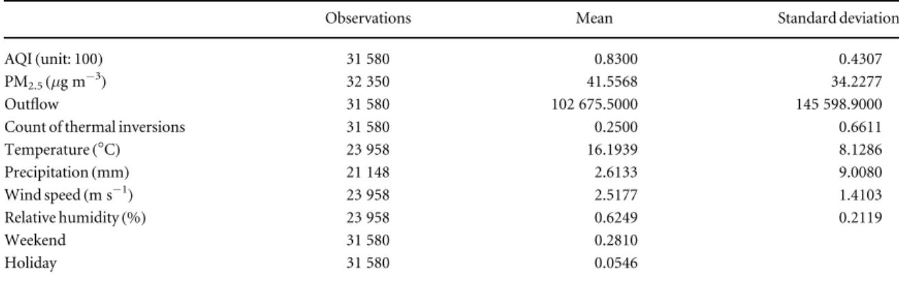
The panel data used in regression models have pas-sed the stationary test for a robust analysis. Descriptive statistics of the data used are shown in table1.
4. Results and discussion
4.1. The effect of AQI on the outflowsCity residents in China tend to avoid being exposed to pollution by leaving cities with low air quality. The AQI shows a positive impact on outflow in the naïve GLS regressions(table2, model(1)). The endogenous issue between air pollution and population mobility is due to two effects. On the one hand, people crowding into a city may cause pollution because of the increasing activity such as transportation, and people leaving a city may reduce pollution. On the other hand, highly polluted air may lead people toflee the city.
Therefore, population mobility and air pollution have reciprocal causation. Thus, we use the count of thermal inversions as the instrumental variable to solve this problem. As shown in model(3)in table2, the count of thermal inversions is a strong IV for addressing the endogenous problems between air pollution and population outflow, and IV estimation solves the problems that the GLS model fails to do. The IV estimations(with the count of thermal inversions as an effective IV), however, show higher AQI which means poorer air quality, instigating more residents to leave(table 2, model (4)). The results show that an increase of AQI by 100 points causes a 49.60% rise in the outflow. Beyond the air quality, temperature also matters in determining traveling behavior, and pre-sents an inverse-U curve relation with an optimum temperature for population outflow(around 26°C). Days that are either very hot or cold affect residents’ behaviors. Other weather conditions show an insignif-icant impact on residents’outflow behavior, indicating that air pollution is even more powerful in driving people out than bad weather.
4.2. The effect of PM2.5
As the air pollutant that attracts most attention, PM2.5
and its effect have been widely studied(Xieet al2016, Haoet al2018, Majiet al2018, Zhenget al2019). Here, we introduce thermal inversion as a good instrument (table 2, model (5))for working out the impact of PM2.5, since the GLS model for PM2.5shows a negative
effect on outflows (table 2, model (2)). In the IV models, a rise of PM2.5of 1μg m−3may cause a 0.47%
increase in the population outflow(table2, model(6)). PM2.5 shows a similar impact on mobility as AQI,
because in many cities in China PM2.5is the dominant
pollutant, and PM2.5 is highly correlated with AQI
(correlation coefficient 0.5901 withp<0.001). The temperature and wind speed also have an impact on population mobility, and gentle breeze seems to keep residents where they are(table2, model(6)).
4.3. The effect of air quality on previous days Since decisions about traveling are made some time before the trip, air quality on previous days may influence people’s traveling decisions. However, the
Table 1.Descriptive statistics of the data.
Observations Mean Standard deviation
AQI(unit: 100) 31 580 0.8300 0.4307
PM2.5(μg m−3) 32 350 41.5568 34.2277
Outflow 31 580 102 675.5000 145 598.9000
Count of thermal inversions 31 580 0.2500 0.6611
Temperature(°C) 23 958 16.1939 8.1286 Precipitation(mm) 21 148 2.6133 9.0080 Wind speed(m s−1) 23 958 2.5177 1.4103 Relative humidity(%) 23 958 0.6249 0.2119 Weekend 31 580 0.2810 Holiday 31 580 0.0546 4 Environ. Res. Lett.14(2019)124025
influence may vary with the distance and the means of transportation people choose. Air pollution may drive people away from their cities in a short-term period, and theflexibility of road and railway travel in China allows people to choose, change or cancel their journey, while air trips are lessflexible and may be not as sensitive to air pollution. We tested the impact of the AQI 0–7 days before the mobility event on outflow by air, railway and road(table3), and found that the AQI of previous days has no significant impact on air trips(model(1))but certainly influences the mobility by railway(model(2))and road(model(3)). The AQI 3 and 7 days previously positively affects outflow by railway and road, i.e. when the air quality is poor, people tend to choose to leave the city in 3 days or in a week by railway or by road. Whileflight tickets are usually ordered more than a week in advance, the short-term reactions to air pollution are not as significant. Long-term mechanics of the impact of air quality on mobility by air relate to anthropogenic factors, and are out of the range of this work.
4.4. Working days, weekends and holidays
People are more likely to travel for recreational purposes on weekends and holidays than on working days. As recreational trips usually contain more
outdoor activities, the populationflows on holidays may be more affected by air quality. To test such a heterogeneous effect, we added two interactive terms to AQI and dummies indicating the weekends and holidays(including Tomb Sweeping Day and May Day holidays), respectively, into the regression. If the weekend and holiday effect is not considered, the effect of AQI on all dates is as shown in section4.1, i.e. an increase in the AQI causes a larger outflow. However, when dividing the time range, the weekend/holiday effects counteract the general effect, which means on holidays, the equivalent rise in the AQI may lead to fewer residents leaving the city. Generally, a 100 point increase in the AQI leads to a 49.60% increase in outflow(as shown before in table2), but on weekends and holidays that increase in AQI causes an uncertain impact on population outflow. Theoretically, on weekends and holidays, city residents have more time to travel freely. In this regard, their avoidance of air pollution should be more frequent. But 2-day week-ends are only enough for a short-distance round trip, possibly to nearby cities. Legal holidays are no shorter than 3 days. Although compulsory trips still happen on weekends and holidays, spontaneous mobility counts for the largest part. Most people would choose close travel destinations due to budget, convenience
Table 2.Impact of AQI and PM2.5on population outflow mobility.
GLS IV
(1) (2) (3) (4) (5) (6)
Log(outflow) AQI stage 1
Log(outflow) stage 2 PM2.5stage 1 Log(outflow) stage 2 AQI 0.0166*** 0.4960** (0.0036) (0.2325) PM2.5 −0.0003*** 0.0047** (0.0001) (0.0019) Count of thermal inversions 0.0121*** 1.3084*** (0.0040) (0.2851) Temperature2 −0.0001*** −0.0001*** 0.0003*** −0.0003*** 0.0089*** −0.0002*** (0.000 01) (0.000 01) (0.000 03) (0.0001) (0.0023) (0.000 03) Temperature 0.0078*** 0.0083*** 0.0115*** 0.0023 0.8373*** 0.0041** (0.0004) (0.0004) (0.0008) (0.0027) (0.0638) (0.0017) Precipitation −0.0002 −0.0003* −0.0015*** 0.0005 −0.1154*** 0.0003 (0.0002) (0.0002) (0.0002) (0.0004) (0.0144) (0.0003) Relative humidity2 −0.1876*** −0.2355*** −1.3348*** 0.4587 −59.4978*** 0.0704 (0.0308) (0.0304) (0.0731) (0.3154) (7.0206) (0.1221) Relative humidity 0.2480*** 0.3100*** 1.3952*** −0.4279 95.1891*** −0.1760 (0.0378) (0.0376) (0.0949) (0.3317) (9.1527) (0.1899) Wind speed −0.0026** −0.0034*** −0.0057** 0.0003 −2.3329*** 0.0085* (0.0011) (0.0011) (0.0023) (0.0021) (0.1916) (0.0047) Fixed effects
City Yes Yes Yes Yes Yes Yes
Date Yes Yes Yes Yes Yes Yes
Observations 21 094 21 222 21 094 21 094 21 222 21 222
Fstatistic 280.4750*** 106.5675***
R2 0.0212 0.0236 0.0864 0.0028 0.0345 0.0010
GLS, naïve generalized least square models; IV, instrumental variable models. Robust standard errors clustered by city in parentheses.
and time. The mean distance of working-day mobility is larger than that of weekend mobility, which is in turn larger than that of the holidays. (The mean mobility distances on working days, weekends and holidays that are covered in our data are 619.4 km, 599.9 km and 470.3 km, respectively.) These results support the idea that city residents are inclined to choose somewhere close for leisure.
Models(2)and(3)in table4show that the air qual-ity at the weekends and holidays does not have a sig-nificant impact on mobility. Similarly, weather conditions(all as control variables)other than temper-ature show an insignificant effect, indicating their small impact on residents’travel decisions. A possible reason is that city residents may refuse to travel when air quality is poor. Since the destination is near, the air quality there is similar to their place of residence.
Based on intuition and the air quality alerts of their home cities, people may expect that the air quality of the destination will not improve significantly and decide to stay at home on weekends and holidays (Zivin and Neidell2009)—they follow experts’ sugges-tions(Laumbachet al2015)to decline all kinds of out-door activities including traveling to a close city and going out in their own city. On working days, how-ever, the mobility of city residents is mainly for com-mercial purposes, meetings or other unavoidable reasons. Thus, the travel plan is unlikely to be canceled even if the target place is heavily polluted regardless of the distance(as shown in a generally negative impact in table4, models(2)and(3)).
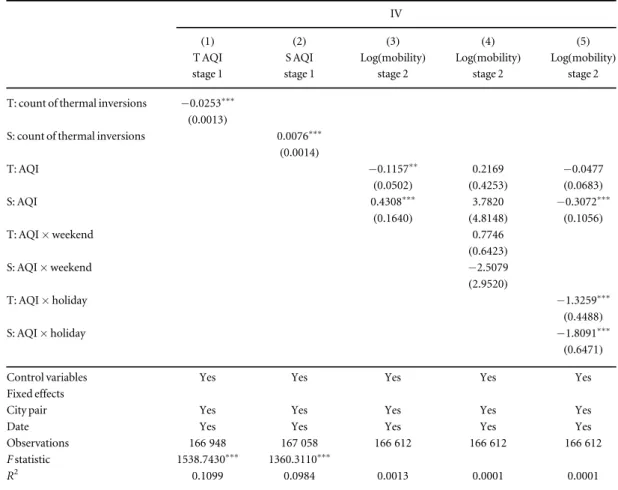
4.5. Gravity model of pairwise populationflows The gravity models of pairwise population flows among cities provide evidence for the relation between air quality and population mobility from a relative viewpoint. The populationflows between city pairs of the source(noted as S)and the target(noted as T)cities present an impact of AQI that is largely consistent with the results above: with the source cities’AQI rising, more residents leave for other cities. Model (3) in table5shows a normal tendency that a higher AQI of the source city and a relatively lower AQI of the target city are conducive to more population flow, which means cleaner air quality attracts people to escape from cities with dirtier air.
To investigate the weekend and holiday effect, we added the interaction of weekend, holiday and AQI. Models(4)and(5)in table5show the inhibitory effect of local air quality on outflows, as discussed above.
Table 3.Impact of AQI of previous days on population outflow by means of transportation. GLS (1) (2) (3) Log( out-flow by air) Log(outflow by railway) Log(outflow by road) AQIt 0.0272 0.0120*** 0.0068 (0.0206) (0.0039) (0.0045) AQIt–1 0.0021 0.0023 0.0013 (0.0218) (0.0041) (0.0045) AQIt–2 −0.0168 0.0047 0.0053 (0.0217) (0.0041) (0.0045) AQIt–3 0.0206 0.0087** 0.0099** (0.0215) (0.0041) (0.0045) AQIt–4 −0.0269 0.0061 0.0068 (0.0215) (0.0042) (0.0045) AQIt–5 0.0177 −0.0003 −0.0026 (0.0215) (0.0042) (0.0045) AQIt–6 0.0174 0.0047 −0.0009 (0.0218) (0.0041) (0.0045) AQIt–7 −0.0061 0.0198*** 0.0111** (0.0203) (0.0039) (0.0043) Temperature2 −0.0001 −0.0002*** −0.0003*** (0.0001) (0.000 02) (0.000 03) Temperature −0.0067** 0.0085*** 0.0156*** (0.0026) (0.0006) (0.0009) Precipitation 0.0005 −0.0002 −0.0005*** (0.0011) (0.0001) (0.0002) Relative humidity2 0.0299 −0.2264*** −0.3111*** (0.1904) (0.0325) (0.0518) Relative humidity −0.1775 0.2842*** 0.3513*** (0.2200) (0.0404) (0.0722) Wind speed 0.0086 −0.0025** −0.0049*** (0.0075) (0.0011) (0.0017) Fixed effects
City Yes Yes Yes
Date Yes Yes Yes
Observations 18 504 18 504 18 504
R2 0.0010 0.0231 0.0263
GLS, naïve generalized least square models; AQIt–n,AQI ndays
before the mobility. Robust standard errors clustered by city in parentheses.*p<0.1;**p<0.05;***p<0.01.
Table 4.Impact of AQI on population mobility during holidays.
IV (1) (2) (3) AQI stage 1 Log( out-flow)stage 2 Log( out-flow)stage 2 Count of thermal inversions 0.0121*** (0.0040) AQI 0.9294 −1.5169 (0.6622) (3.7424) AQI×weekend −0.4450 (0.3673) AQI×holiday −18.0961 (45.5097) Control variables Yes Yes Yes Fixed effects
City Yes Yes Yes
Date Yes Yes Yes
Observations 21 094 21 094 21 094
Fstatistic 280.4750***
R2 0.0864 0.0017 0.0001
IV, instrumental variable models. Robust standard errors clustered by city in parentheses.*p<0.1;**p<0.05;***p<0.01. Control variables: weather conditions.
6 Environ. Res. Lett.14(2019)124025
However, there are rather controversial effects on weekends and holidays. Model(5)in table5shows that the AQI of the destination on holidays motivated peo-ple to travel, and the attractiveness of target cities’ clean air is effective and becomes even larger than on
‘non-holiday’days(table5, model(3))because people consider the environment more since it is a precious holiday trip. However, from the view of source cities, similar to discussions in section 4.4, counteractive effects between leaving and staying indoors exist and the total avoidance of exposure to pollutants prevails. The source cities with poor air quality would tend to lose their residents. However, the impact of air quality on theflow between two cities varied among different time periods due to residents’different responses to air pollution. Shorter mobility distance on holidays tends to be accompanied by a greater tendency to stay indoors.
5. Conclusion
China faces severe air pollution issues following the rapid growth of the economy, and recent studies have noted that the health, productivity and activity of Chinese urban residents can be influenced by air quality. People tend to make avoidance behaviors when the air quality is bad, including reducing
outdoor activities, traveling or migrating. Revealing the relation between air quality and population mobility is helpful for a more accurate estimation of the health risks of exposure to pollution, a better calculation of economic or productivity gain and loss, and more comprehensive guidance for city environ-mental management. However, few studies have focussed on this question. This study intends to solve the question of how air quality affects population mobility by using IV regressions with daily city data (including smartphone-based data). Results show that air quality does affect the population outflows of cities. When the AQI of a city rises by 100 points, the population outflow increases by 49.60%. Taking PM2.5 as the air quality variable, we obtain similar
results to the AQI, and a rise of 1μg m−3in PM2.5may
cause a 0.47% increase in the population outflow. Air pollution on one day may drive people to leave the city 3 days or a week later, going to other cities by railway or by road. There are heterogeneous effects among time ranges and cities. On weekends and holidays, city residents tend to take avoidance actions with air pollution, but it seems that the effect of staying indoors counteracts the leaving effect.
Based on the results above, this study can provide clues for making more accurate estimations of health risks considering the population mobility issue. The
Table 5.Impact of AQI on source–target mobility between city pairs.
IV
(1) (2) (3) (4) (5)
T AQI S AQI Log(mobility) Log(mobility) Log(mobility) stage 1 stage 1 stage 2 stage 2 stage 2
T: count of thermal inversions −0.0253***
(0.0013)
S: count of thermal inversions 0.0076***
(0.0014) T: AQI −0.1157** 0.2169 −0.0477 (0.0502) (0.4253) (0.0683) S: AQI 0.4308*** 3.7820 −0.3072*** (0.1640) (4.8148) (0.1056) T: AQI×weekend 0.7746 (0.6423) S: AQI×weekend −2.5079 (2.9520) T: AQI×holiday −1.3259*** (0.4488) S: AQI×holiday −1.8091*** (0.6471)
Control variables Yes Yes Yes Yes Yes
Fixed effects
City pair Yes Yes Yes Yes Yes
Date Yes Yes Yes Yes Yes
Observations 166 948 167 058 166 612 166 612 166 612
Fstatistic 1538.7430*** 1360.3110***
R2 0.1099 0.0984 0.0013 0.0001 0.0001
IV, instrumental variable models. S, source city; T, target city. Robust standard errors clustered by city in parentheses.*p<0.1;
outflow of a city should be considered in the exposure estimation. Also, the evaluation of the economic loss due to air pollution, for example loss of tourism and productivity, can be improved by taking the pollution-caused population outflow into account. However, the most valuable aspect of the results is that in addition to reasons of health and civic responsibility, cities now have another key reason to protect the atmospheric environment. As more cities are becoming developed cities, residents are more able to selecting a pleasant city in which to live. A city with poor air quality not only loses visitors but talented people also leave tofind another workplace. The time range matters in resi-dents’responses to air quality—weekends and holi-days give residents the choice of staying indoors to avoid exposure to air pollution. If more residents choose to stay indoors in polluted cities on weekends and holidays, not only tourism but other local eco-nomic activities would decline due to fewer residents going outdoors. The outflows due to air pollution may also influence the city transportation system, which could either be under pressure or insufficiently uti-lized. Furthermore, judging by our short-term results, commercial mobility may also be influenced by air quality, which is important for non-tourist cities because they need to attract talent or investment. Our
findings are consistent with the long-term migration response to air quality(Chenet al2017), which indi-cates a trend of people leaving due to bad air quality. Civic governments need to rethink the importance of air quality, and more effective environmental manage-ment policies should be implemanage-mented for better reten-tion of residents and visitors.
This study has limitations. The impact of season-ality of air quseason-ality and thermal inversions has been checked, and would not significantly influence the effectiveness of the IV methods(for details, see the supplementary materials available online atstacks.iop. org/ERL/14/124025/mmedia). However, there remains a seasonality issue between population mobi-lity and thermal inversions due to the short range of mobility data. So we used monthly passenger capacity data tofind that in the period of March to June mobi-lity showed no consistent seasonamobi-lity with thermal inversions. This result cannot eliminate the seasonality issue between mobility and thermal inversions but suggests a weak influence that may not affect the robustness of the results. In addition, the relatively short time range may not be sufficient to reveal the complete impact of air pollution on holidays, but our interpretation of the holiday effect can still be con-sidered. Because the data only covered outflows, we did not discuss the sensitivity of inflows to air quality changes. Future work could use data that cover a longer period and more cities to confirm the casualty and explore further issues with multiple models.
Acknowledgments
This paper isfinancially supported by the National Key Research and Development Program of China (no. 2018YFC0214001)to Ping Kang, the National Natural Science Foundation of China(41601484)to Chaogui Kang and the Startup Fund for Distinguished Scholars of Huazhong Agricultural University to Zhen Wang.
Data availability statement
The data that support thefindings of this study are available from Z Wang upon reasonable request.
ORCID iDs
Can Cui https://orcid.org/0000-0001-9766-9912 Zhen Wang https://orcid.org/ 0000-0002-7902-4093
Pan He https://orcid.org/0000-0003-1088-6290
References
Arceo E, Hanna R and Oliva P 2016 Does the effect of pollution on infant mortality differ between developing and developed countries? Evidence from Mexico cityEcon. J.126257–80
Bayer P, Keohane N and Timmins C 2009 Migration and hedonic valuation: the case of air qualityJ. Environ. Econ. Manage.58
1–14
Bresnahan B W, Dickie M and Gerking S 1997 Averting behavior and urban air pollutionLand Econ.73340
Chen S, Oliva P and Zhang P 2017The Effect of Air Pollution on Migration: Evidence from China(Cambridge, MA: National Bureau of Economic Research)
China Ministry of Environment Protection 2016Technical Regulation on Ambient Air Quality Index(on trial) (Beijing: China Ministry of Environment Protection)pp 2–4 Forouzanfar M Het al2016 Global, regional, and national
comparative risk assessment of 79 behavioural, environmental and occupational, and metabolic risks or clusters of risks, 1990–2015: a systematic analysis for the Global Burden of Disease study 2015Lancet3881659–724
Fu S, Viard V B and Zhang P 2017 Air Pollution and Manufacturing
firm Productivity: Nationwide Estimates for ChinaSSRN (https://doi.org/10.2139/ssrn.2956505)
Hao Y, Peng H, Temulun T, Liu L-Q, Mao J, Lu Z-N and Chen H 2018 How harmful is air pollution to economic development? New evidence from PM2.5 concentrations of Chinese cities
J. Clean. Prod.172743–57
Katsoulis B D 1988 Some meteorological aspects of air pollution in Athens, GreeceMeteorol. Atmos. Phys.39203–12
Laumbach R, Meng Q and Kipen H 2015 What can individuals do to reduce personal health risks from air pollution?J. Thorac. Dis. 796–107
Maji K J, Ye W-F, Arora M and Shiva Nagendra S M 2018 PM2.5-related health and economic loss assessment for 338 Chinese citiesEnviron. Int.121392–403
MihaličT 2000 Environmental management of a tourist destination
Tourism Manage.2165–78
National Bureau of Statistics of China 2018China Statistical Yearbook 2018(Beijing: China Statistics Press)p 33 National Centers for Environmental Prediction, National Weather
Service, NOAA and US Department of Commerce 2000 NCEP FNL Operational Model Global Tropospheric Analyses, continuing from July 1999Research Data Archive
8 Environ. Res. Lett.14(2019)124025
(Boulder, CO: National Center for Atmospheric Research)
((https://doi.org/10.5065/D6M043C6))
Qin Y and Zhu H 2018 Run away? Air pollution and emigration interests in ChinaJ. Population Econ.31235–66
Rohde R A and Muller R A 2015 Air pollution in China: mapping of concentrations and sourcesPLoS One10e0135749
Saberian S, Heyes A and Rivers N 2017 Alerts work! Air quality warnings and cyclingResour. Energy Econ.49165–85
Song P, Zhang X, Huang Q, Long P and Du Y 2019 Main forecasting models and applications of urban ambient air quality in ChinaSichuan Environ.3870–6
Welch E, Gu X and Kramer L 2005 The effects of ozone action day public advisories on train ridership in ChicagoTransport. Res.
D10445–58
Xie Y, Dai H, Dong H, Hanaoka T and Masui T 2016 Economic impacts from PM2.5pollution-related health effects in china:
a provincial-level analysisEnviron. Sci. Technol.504836–43
Zavattero D A, Ward J A and Strong C K 1998 Air quality effects of travel changesTransport. Res. Rec.164189–96
Zheng S, Zhang X, Song Z and Sun C 2016 Influence of air pollution on urban residents’outdoor activity: empirical study based on dining-out data from the Dianping websiteJ. Tsinghua Univ. (Sci. Technol.)5689–96
Zheng S, Wang J, Sun C, Zhang X and Kahn M E 2019 Air pollution lowers Chinese urbanites’expressed happiness on social mediaNat. Hum. Behav.3237–43
Zivin J G and Neidell M 2009 Days of haze: environmental information disclosure and intertemporal avoidance behaviorJ. Environ. Econ. Manage.58119–28