The Dynamics of Economic Functions: Modelling and
Forecasting the Yield Curve
Clive G. Bowsher
∗Nu
ffi
eld College, Oxford University
Roland Meeks
†Federal Reserve Bank of Dallas
March 28, 2008
Abstract
The class of Functional Signal plus Noise (FSN) models is introduced that provides a new, general method for modelling and forecasting time series of economic functions. The underlying, continuous economic function (or ‘signal’) is a natural cubic spline whose dynamic evolution is driven by a cointegrated vector autoregression for the ordinates (or ‘y-values’) at the knots of the spline. The natural cubic spline provides flexible cross-sectional fit and results in a linear, state space model. This FSN model achieves dimension reduction, provides a coherent description of the observed yield curve and its dynamics as the cross-sectional
dimensionNbecomes large, and can feasibly be estimated and used for forecasting whenNis large. The
integration and cointegration properties of the model are derived. The FSN models are then applied to forecasting 36-dimensional yield curves for US Treasury bonds at the one month ahead horizon. The method consistently outperforms the Diebold and Li (2006) and random walk forecasts on the basis of both mean square forecast error criteria and economically relevant loss functions derived from the realised profits of pairs trading algorithms. The analysis also highlights in a concrete setting the dangers of attempts to infer the relative economic value of model forecasts on the basis of their associated mean square forecast errors.
Keywords: FSN-ECM models, functional time series, term structure, forecasting interest rates, natural cubic spline, state space form.
JEL classification: C33, C51, C53, E47, G12.
1
INTRODUCTION
This paper develops a novel econometric framework for modelling and forecasting time series of economic functions. In financial economics, market prices at a given point in time are a function of the characteristics of the asset traded such as its maturity date, transaction volume or strike price. It is often appropriate to consider the underlying price as a continuous function of these characteristics. Prominent examples include the zero-coupon yield curve, the ask and bid (or inverse demand and supply) curves of the limit order book of a financial exchange, and the implied volatility surface of options prices. Despite the importance of such functions there has been little development of general methods to study their dynamics that are applicable and feasible when the cross-sectional dimension of the data is moderate or large. To address this need we introduce Functional Signal plus Noise models and demonstrate their usefulness in the concrete setting of modelling and forecasting zero-coupon yield curves. The vast majority of empirical dynamic studies of the yield curve concentrate on a small subset of bond maturities as a result of the econometric difficulties
∗
Corresponding author: Nuffield College, Oxford OX1 1NF, [email protected], tel:+44 (0)1865 278969, fax: +44 (0)1865 278621. Functional Signal plus Noise (FSN) models first appeared in the earlier working paper, Bowsher (2004).
†
Research Department, Federal Reserve Bank of Dallas, 2200 N. Pearl St., Dallas TX 75201, [email protected], tel:+1 214 922 6804. The views expressed in this paper are not necessarily those of the Federal Reserve Bank of Dallas or the Federal Reserve System.
involved in modelling dynamic panel data in which cross-sections consist of functionally related observations. By contrast, our approach is based on a continuous, smooth underlying yield curve (or ‘signal’ function) that is observed with measurement error (or ‘noise’). The Functional Signal plus Noise models appear to be the first systematically to outperform a random walk for the yield curve when forecasting one month ahead, a horizon that has particularly challenged previous forecasting methods.
The main contributions of the paper may be summarised as follows. First, the class of Functional Signal plus Noise (FSN) models is introduced that provides a new, general method for modelling and forecasting time series of economic functions. The underlying continuous, smooth economic function (or ‘signal’) is a natural cubic spline whose dynamic evolution is driven by a cointegrated VAR for the ordinates (‘y-values’) at the knots of the spline. The natural cubic spline provides flexible cross-sectional fit and results in a linear state space model. Since the model’s state equation is the cointegrated VAR written and parametrised in Error Correction form (see Johansen 1996), we call it the FSN-ECM model. This model achieves dimension reduction, provides a coherent description of the observed price or yield curve and its dynamics as the cross-sectional dimensionNbecomes large, and can feasibly be estimated and used for forecasting whenNis large. Second, under the assumption that themknot ordinates (or yields) follow a cointegrated I(1) process with cointegrating rankr, a theorem is derived showing that the observed and latent yield curves of the FSN-ECM process with dimensionN are I(1) processes with cointegrating rank [N−(m−r)]. Third, the FSN-ECM
models are applied to forecasting 36-dimensional yield curves for US Treasury bonds at the one month ahead horizon. The method consistently outperforms both the widely used Diebold and Li (2006) and random walk forecasts on the basis of both mean square forecast error (MSFE) criteria and economically relevant loss functions derived from the realised profits of pairs trading algorithms that each period construct an arbitrage portfolio of discount bonds. Yield spreads are found to provide important information for forecasting the yield curve, but not in the manner prescribed by the Expectations Theory. The analysis also highlights in a concrete setting the dangers of attempts to infer the relative economic value of model forecasts on the basis of their associated MSFEs.
The work presented is a contribution to functional time series analysis. Each yield curve, for example, may be regarded as a finite dimensional vector, albeit of moderately or very high dimension. However, the standard approaches of multivariate time series or panel data analysis are of little help in this setting owing to the cross-sectional dimension (preventing e.g. the standard use of cointegrated VARs) and the close, functional relationship between the yields. Indeed, the analysis of time series of stochastic, continuous functions is in a state of relative infancy. Previous work in the statistics literature includes the use of Functional
AutoRegressive (FAR) models for forecasting entire smooth, continuous functions by Besse and Cardot (1996) and Besse, Cardot, and Stephenson (2000). Kargin and Onatski (2007) develop a new technique, the predictive factor decomposition, for estimation of the autoregressive operator of FARs. The method is applied to the point prediction at a three month horizon of cubic spline interpolations of the term structure of Eurodollar futures rates, but is found to have uniformly larger MSFEs across a wide range of maturities than the Diebold and Li (2006) forecasting method that is implemented.
Our FSN-ECM models may be interpreted as a special type of dynamic factor model (see Stock and Watson 2006, p. 524) in which the ordinates (yields) at the knots of the spline are the factors and the factor loadings are determined by the requirement that the signal function (i.e. the ‘common component’) be a natural cubic spline, rather than the factor loadings being parameters for estimation. The semiparametric FSN approach thus allows quasi-maximum likelihood estimation and prediction using a linear state space form and the filtering methods of Jungbacker and Koopman (2007), even when the cross-sectional dimension (N) of the data is very large. Our method may be contrasted with non-parametric approaches to estimation of factor models using either static or dynamic principal components in which asymptotic consistency is established for both large cross-sectional dimensionNand large number of time series observationsT(see Boivin and Ng 2005 for discussion of these methods from a forecasting perspective). Of course, parametric and non-parametric approaches are complementary and have well-established relative advantages and disadvantages. In the context of modelling economic functions, the FSN-ECM approach exploits thea prioriinformation that the cross-section consists of (noisy) observations of a continuous, smooth underlying function. Furthermore, the FSN-ECM approach is applicable to panels with only moderate cross-sectional dimension.
A recurring theme in the term structure literature is the considerable difficulty of outperforming na¨ıve forecasting devices, particularly the random walk for the yield curve or ‘no change’ forecast (denoted RWYC).
Since this difficulty has been found to be particularly pronounced for one month ahead forecasts and term structure forecasting models are almost always specified at a monthly frequency, our study focuses on forecasting the yield curve at the one month horizon. Diebold and Li (2006) introduced a dynamic version of the Nelson and Siegel (1987) yield curve in which the three parameters or factors describing the curve each follow an AR(1) process. The method is now widely used. However, Diebold and Li (2006) report only comparable forecasting performance to RWYC in terms of mean square forecast errors (MSFEs) at the one month ahead horizon. De Pooter, Ravazzolo, and van Dijk (2007) tried several variants of this forecasting method, but were unable to improve its average root MSFE performance. Almost none of the currently popular term structure forecasting methods that they implemented resulted in lower average root MSFE
than the RWYCat the one month horizon, and the inclusion of macroeconomic information resulted in only marginal reductions in average root MSFE at best. Several studies have assessed the forecasting performance of affine term structure models using only a small number of yields. Duffee (2002) finds that forecasts made using the standard class of (‘completely’) affine models typically perform worse than the RWYC even at horizons of 3, 6 and 12 months ahead. His ‘essentially affine’ models produce forecasts somewhat better than the RWYCfor the three maturities reported and at these three horizons. Ang and Piazzesi (2003) present a
VAR model in the affine class for yields of five different maturities which imposes no-arbitrage restrictions and performs only slightly better than the RWYCat the one month ahead horizon for four of the five maturities
used. Incorporating macroeconomic factors in the model improves the forecast performance for those four maturities.
For the first time in the literature, we present forecasting models that consistently outperform a random walk for the yield curve at the one month horizon, both under MSFE-based crtieria and ones based on realised trading profits. Furthermore, a broad range of 36 different maturities is used in the forecast evaluation exercise. The structure of the paper is as follows. Section 2 introduces the new class of FSN-ECM models and states a theorem on their integration and cointegration properties in Section 2.2. The choice of a natural cubic spline for the continuous, economic signal function is motivated in Section 2.3 in terms of the good interpolating and approximation properties of such splines. The use of cubic splines in term structure estimation is reviewed and it is argued that potential criticisms in terms of their extrapolatory behaviour misunderstand their role here as piecewise, local approximations. Section 3 presents the specification and selection of FSN-ECM forecasting models for the zero-coupon yield curve and compares their out-of-sample performance to rival models using MSFE-based criteria. Section 4 considers forecast evaluation under economically relevant loss functions derived from the realised profits of pairs trading algorithms, whilst Section 5 concludes. The Appendix provides the necessary mathematical details on natural cubic spline functions so that the paper is self-contained. These are denoted here as a function ofτbyS(τ).
2
FUNCTIONAL SIGNAL PLUS NOISE MODELS
Functional Signal plus Noise (FSN) models provide a general method for modelling and forecasting time series of economic functions. Such a method must have the ability to fit flexibly the shape of the cross-sectional data whilst providing an accurate description of the dynamics of the time series. The FSN models employ a natural cubic spline to model the underlying, continuous economic function, the dynamic evolution of which is driven by a cointegrated Vector AutoRegression (VAR) or Error Correction Model (ECM) of relatively small
dimension. The natural cubic spline is expected to provide the property of good cross-sectional fit in a wide range of settings as a result of its desirable properties as an approximating and interpolating function. The use of the cointegrated VAR ensures that the dynamic properties of both the state (or ‘factor’) and observation vectors are well understood. Furthermore, since cointegrated VARs have been very successful as models of financial variables that may be written in terms of log prices, their incorporation is likely to result in good empirical performance. The resultant FSN-ECM model combines the virtues of parsimony and parametric interpretability. The method is applicable when the underlying economic function is believed to be smooth and, in heuristic terms, varies such that its general shape can be described by a vector of ordinates (‘y-values’) of relatively small dimension. The method then exploits the dimension-reduction property inherent in the functional data. For concreteness, the exposition below is given in terms of yield curves but is general in scope. For example, Bowsher (2004) provides an application of FSN models to the bid and ask curves of the electronic limit order book of a financial exchange.
A zero-coupon or discount bond with face value $1 and maturity τ is a security that makes a single payment of $1τperiods from today. Itsyield to maturity yt(τ) is defined as the per period, continuously
compounded return obtained by holding the bond from timettot+τ, so that
yt(τ)=−τ−1pt(τ), (1)
wherept(τ) is the log price of the bond att. The (zero-coupon)yield curveconsists of the yields on discount
bonds of different maturities and is denoted here by the vectoryt(τ) :=(yt(τ1),yt(τ2), ...,yt(τN))0.We develop
methods for the empirically important case where the cross-sectional dimension Nof the observed yield curve is too large to allow the use of standard, multivariate time series methods. In Section 3 the task will be to forecast one month ahead a 36-dimensional yield curve withτ=(1.5,2,3, ...,11,12,15,18, ...,81,84) and maturities measured in months. A 3-dimensional plot of the dataset used there may usefully be previewed at this stage by examining the first panel of Figure 2. The plot strongly suggests the suitability of treating each observed yield curve as a smooth function perturbed by noise. (Taking the contemporaneous pairwise correlations of yields for adjacent maturities using the dataset shown there gives correlations that all lie between 0.9964 and 0.9997). The FSN models proposed below have exactly this form and capture the functional, cross-sectional relationship between contemporaneous observations (yields) by modelling the observed curves as the sum of a smooth, latent ‘signal function’S(τ) and noise.
2.1
FSN-ECM models
The signal function used is a natural cubic spline uniquely determined by the ordinates (yields) that correspond to the knots of the spline,γt. The state equation of the FSN model then determines the stochastic evolution of the spline function by specifying thatγ
tfollows a cointegrated VAR (or ECM). The resultant
FSN-ECM model may be written in linear state space form, thus allowing the use of the Kalman filter to compute both the Gaussian quasi-likelihood function and 1-step ahead point predictions. Harvey and Koopman (1993) were the first to describe a linear state space model with a state equation determining the stochastic evolution of a cubic spline function. There, as in Koopman and Ooms (2003), the stochastic spline is used to model the latent, time-varying periodic pattern of a scalar time series. This contrasts the present work in which the stochastic splines are used as a tool in functional time series analysis and assume the role of smooth approximations to the observed functional data. The termKalman filteris taken here to refer to the recursions as they are conveniently stated in Koopman, Shephard, and Doornik (1999, Section 4.3, pp. 122-123). For a textbook exposition of the Kalman filtering procedure, see Harvey (1989, Ch. 3).
A natural cubic spline (NCS) is essentially a piecewise cubic function with pieces that join together to form a twice continuously differentiable function overall (see Appendix B). The NCS signal function or latent yield curve evaluated at the maturitiesτis written asSγ
t(τ) :=(Sγt(τ1), ...,Sγt(τN))
0
. The NCS hasm knots positioned at the maturitiesk=(1,k2, ...,km) which are deterministic and fixed over time. The notation Sγ
t(τ) is used to imply that the spline interpolates to the latent yieldsγt = (γ1t, ..., γmt)
0
– i.e. Sγ
t(kj) = γjt
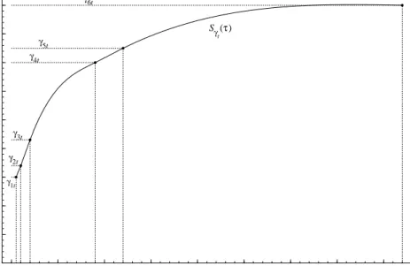
for j =1, ...,m.We refer to the vectorγt as theknot-yieldsof the spline. An illustrative NCS signal function
is shown in Figure 1. Another terminology is to refer toSγ
t(τ) as a NCS on (k;γt), since the spline passes through the points (kj, γjt)mj=1,which together determine the remainder of the spline function uniquely. The
vectorskandτneed not have any elements in common and, in the context of FSN-ECM models, the knot vector typically has much smaller dimensionmthan the number of maturitiesN.
A formal definition of the FSN(m)-ECM(p) model now follows, wheremis the number of knots and the pth lag ofγt+1is the maximum lag that enters the ECM state equation. Without loss of generality, we focus on the casep≤2 for expositional simplicity. The definition is stated for the case where the maturitiesτfor which yields are observed in the data are constant over time. Extension to allow for a deterministic, time-varying maturity vectorτtis straightforward both conceptually and computationally (even when its dimension varies over time), but this is not needed in the sequel.
Definition 1 FSN(m)-ECM(2)Model. Let the vector of observed maturities beτ=(τ1, ..., τN), withτ1 ≥ k1 =1
Figure 1: An illustrative NCS signal function or latent yield curve,Sγ t(τ). 0 10 20 30 40 50 60 70 80 1 2 3 4 5 6 7 8 9 Sγ t (τ) γ5t γ4t γ3t γ2t γ6t γ1t maturity
Note: The yields at the knots, γjt, are labelled and plotted using filled circles; the knots are given byk =
(1,2,4,18,24,84). given by yt(τ) = Sγt(τ)+εt(τ) = W(k,τ)γt+εt(τ), (2) ∆γt+1 = α(β0γt−µ)+Ψ∆γt+νt, (3) for t = 1,2, ...HereSγ
t(τ)is a natural cubic spline on(k;γt),the N×m deterministic matrixW(k,τ)is given by
Lemma 7 of the Appendix, and bothαandβare m×r matrices with rank equal to r< m. LettingAγ(z)denote the
characteristic polynomial for the process{γt}, it is imposed that|Aγ(z)|=0implies that|z|>1or z=1.
The initial state (γ01,γ00)0has finite first and second moments given byγ∗ andΩ∗ respectively.The series{ut :=
(εt(τ)0,νt0)0}has a finite second moment for all t and satisfies, for all t,E[ut]=0,E[εt(τ)εt(τ)0]=Ωε,E[νtνt0]=Ων,
E[εt(τ)νt0
] = 0,E[utus0] = 0∀s , t, andE[ut(γ01,γ00)] = 0. Note that {ut}is a vector white noise process. The
parameters of the model are thus(α,β,µ,Ψ,Ων,Ωε).
The Gaussian FSN(m)-ECM(2) Model has the additional condition imposed that bothut and (γ01,γ00)0 have
multivariate Normal distributions.
The choice of a NCS as the signal function or latent yield curveS(τ) is discussed in detail in Section 2.3 below, and stems from the desirable properties that the NCS has as a smooth approximating and interpolating function. Note that the latent signal function is expected to be smoother than the observed ‘curve’ yt(τ)
and captures the underlying economic function of interest. The ECM state equation (3) is motivated by the numerous studies that successfully model a relatively small vector of yields using a cointegrated VAR in
which the process for the yields, here{γ
t}, isI(1) and{β 0
γt−µ}is a stationary, mean zero vector of cointegrating
relations. Given the reduced rankr<mof bothαandβimposed by Definition 1, a necessary and sufficient condition forγt to have these properties is that det[α0
⊥(I−Ψ)β⊥] , 0. Note that then µ = E[β 0
γt] is the stationary mean of the cointegrating relations andE[∆γt+1]=0,thus excluding deterministic trends.
The FSN-ECM model combines the virtues of parsimony and parametric interpretability. Dimension reduction is achieved provided thatmNand the approach remains feasible as the cross-sectional dimension
N of the observed yield curve becomes large. Consider varying the vector of observed maturities τ in Definition 1 by increasingNbut holding the maximum observed maturityτNfixed so that the yield curve is
‘filled in’. Since the ECM state equation remains unchanged when the model is well-specified, and provided that the latent signal function captures all or most of the cross-sectional dependence (e.g. the number of parameters inΩεdoes not vary withN), the FSN-ECM model continues to provide a parsimonious forecasting
model. Jungbacker and Koopman (2007) provide new, computationally efficient methods for implementing the Kalman filter for dynamic factor models that are applicable to the FSN-ECM model and are ideally suited to the largeNmcase just described. QML estimation and prediction for the FSN-ECM model thus remain
computationally feasible in this case. Using the FSN-ECM forecasting models described in Section 3.2, we would expect the method to be computationally feasible for, say,N≈5000.
The Expectations Theory (ET) of the term stucture implies for anI(1),m-dimensional vector of observed yields that the cointegrating rankris (m−1) and that (m−1) linearly independent yield spreads are
coin-tegrating relations. These hypotheses have received considerable attention in the cointegration-based yield curve literature (seeinter aliaHall, Anderson, and Granger 1992, Shea 1992 and Pagan, Hall, and Martin 1996) with the findings supportingr=(m−1) orr=(m−2) and cointegrating relations that can be written as linear
combinations of yield spreads. There is a tendency to reject the implications of the ET using hypothesis testing techniques based on asymptotic critical values. However, it is important to pay attention to the validity of the critical values used. For example, Pagan, Hall, and Martin (1996) report rejection of the standard hypothesis test but note that the point estimates obtained are quite close to the situation where the cointegrating relations implied by the ET hold. They highlight the major impact on the critical values of a levels effect of the short rate in the disturbance of the VAR, which may result in the test rejecting erroneously. More generally, the conclusions of in-sample hypothesis testing do not necessarily carry over to the context of out-of-sample forecasting using potentially mis-specified models.
The ECM state equation has the advantage that the dynamic properties of both the knot-yieldsγtand the yield curves are well understood. The following section derives the integration and cointegration properties
of the latent and observed yield curves of an FSN-ECM process.
2.2
FSN-ECM model dynamics
We begin from the empirically well-motivated assumption that the process for themknot-yields{γt}is a
cointegratedI(1) process and prove that the latent and observed yield curves are also then cointegratedI(1) processes with cointegrating rank [N−(m−r)], wherer=rank(α)=rank(β). The (m−r) common trends of
the knot-yields, and of the latent and observed yield curves are identical and given byα0 ⊥
Pt
i=1νi. (Whenδis
ann×rmatrix of full rank, we use the notationδ⊥for somen×(n−r) matrix of full rank such thatδ0δ⊥=0).
Theorem 2 (Integration and Cointegration Properties of FSN-ECM Model)Letyt(τ)follow an FSN(m)-ECM(2)
process withdet[α0⊥(I−Ψ)β⊥],0.Then{γt}is I(1)and{β
0
γt−µ}is a stationary, mean zero vector of cointegrating
relations. It follows from Definition 1 that the processes for the observed and latent yield curves,{yt(τ)}and{Sγ
t(τ)}t=1,2,...
resp., are I(1)cointegrated processes with the matrix of cointegrating vectors given byφ=[W(k,τ)β⊥]⊥in both cases.
The cointegrating rank is thus equal torank(φ)=N−(m−r)in both cases.
Proof. The necessity and sufficiency of the condition det[α0
⊥(I−Ψ)β⊥],0follows directly from Theorem
4.2 of Johansen (1996), as does the moving average (MA) representation γt=C
t
X
i=1
νi+B(L)(νt−αµ)+D, (4)
whereDdepends on initial values such thatβ0D = 0,C= β⊥[α0
⊥(I−Ψ)β⊥] −1α0
⊥, and the power series for
B(z) is convergent for|z|<1+δfor someδ >0.
We thus have the following MA representation for the latent yield curve
Sγ t(τ)=W(k,τ)C t X i=1 νi+W(k,τ)B(L)(νt−αµ)+W(k,τ)D. (5)
Notice that rank[W(k,τ)] = mand rank[W(k,τ)C] = m−r > 0. In particular, W(k,τ)C , 0. It follows
immediately that bothSγ
t(τ) andyt(τ)=Sγt(τ)+εtareI(1) processes (since the sum of anI(1) process and an
I(0) process is itselfI(1)).
Note also that W(k,τ)β⊥ has full rank equal to (m−r) and hence rank(φ) = N−(m−r). The process {φ0Sγ t(τ)}isI(0) sinceφ 0 W(k,τ)C=φ0W(k,τ)D=0and hence φ0Sγ t(τ)=φ 0 W(k,τ)B(L)(νt−αµ). (6)
The process{φ0yt(τ)}is alsoI(0) sinceE[εtνs0
]=0 ∀s,t.
For a particular choice ofβthe matrix of cointegrating vectors for the yield curve may thus be computed asφ =[W(k,τ)β⊥]⊥. The simple case whereβ
0
γt consists of the (m−1) spreads between the knot-yields is
Example 3 (FSN-ECM Model with Stationary Yield Spreads)Consider the case of the FSN(m)-ECM(2)process in
Theorem 2 with the m×(m−1)matrixβset toβswhereβ0sγt =(γj+1,t−γjt)mj=−11is the stationary vector of spreads between
the knot-yields. ThenW(k,τ)β⊥is an N-vector with all elements identical and we can takeφ0yt(τ)=[yt(τi)−yt(τ1)]Ni=2.
Thus, e.g. whenτ1=1, the observed spreads[yt(τi)−yt(1)]Ni=2are a stationary vector for any N.
2.3
Cubic Spline Signal Functions
We motivate here the choice of a natural cubic spline for the economic signal function or latent yield curve
S(τ),and discuss the use of cubic splines in term structure estimation. A spline may usefully be viewed as a
set of polynomial pieces each of which is alocalapproximation to the function of interest, with the polynomial pieces joined together to form a smooth function overall. Spline functions are a centrepiece of the modern theory that deals with the numerical approximation of functions (see Powell 1996). Cubic splines are used frequently in practice since they provide a balance between accurate approximation and smoothness.
Suppose that a latent yield curve y∗(τ) is inC2[1,km]. Then it is known (see Powell 1996, Theorem 20.3)
that the least maximum or ‘minimax’ error achievable by a cubic spline approximation to y∗(τ) on [1,km],
with arbitrary number and positioning of knots, has the upper bound 3h2sup τ∈[1,km]
{y00
∗(τ)} whereh is the
maximum interval between adjacent knots. Thus the family of cubic splines is able, using a twice continuously differentiable spline function, to approximate y∗(τ) to any required accuracy by using a sufficiently large
number of knots (perhaps spaced uniformly, although this is usually sub-optimal). This approximation ability of cubic splines motivates their use as the signal function in FSN models. A question of importance in the forecasting context is then whether sufficiently accurate cross-sectional fit can be achieved using a number of knots that also allows formulation of a parsimonious FSN-ECM model, a question that we are able to answer strongly in the affirmative in what follows when forecasting the yield curve.
A slightly different way to motivate the use of a natural cubic spline as the latent, smooth economic function in the FSN-ECM model is as follows. Suppose that the ‘true’ latent yields attcorresponding to the maturities k = (1,k2, ...,km) are known to beγt = (γ1t, ..., γmt)0 and one seeks an interpolating function S(τ)∈ C2[1,k
m] that passes through the points (kj, γjt)mj=1. Then it is known that, ofallfunctions inC2[1,km],the
one that minimises the roughness penaltyR1km[S00(τ)]2dτis the NCSSγ
t(τ) (see Powell 1996, Theorem 23.2). In this sense, the NCS is theleastrough or ‘oscillatory’ choice. If the latent economic function is believed to be smooth and its ‘general shape’ can be described by a vector of ordinatesγtof relatively small dimension, then a NCS interpolating between theγjtis a good way to describe the function. Problems would arise if the latent
economic functions vary rapidly over certain maturity ranges and those ranges also change significantly over time, thus necessitating a large number of knotsmto avoid oversmoothing. Such a largemwould then result
in too many parameters associated with the ECM state equation for the FSN-ECM method to be useful for forecasting, unless very long time series were available.
Under the conditions of Definition 1, the FSN-ECM model can be written inlinearstate space form (see Harvey 1989, pp. 100-104) since the deterministic matrixW(k,τ) depends only on the vector of maturitiesτ and the knot positionsk, thus allowing the NCS signal functionSγ
t(τ) to be written as the linear function
W(k,τ)γtof the knot-yields. This is a further advantage of the use of a NCS in the FSN-ECM model since the linear state space form enables use of the Kalman filter to perform both quasi-maximum likelihood estimation (QMLE) and 1-step ahead, linear point prediction. The state vector attcan be taken to be (γ0
t,γ 0 t−1) 0 or, in an isomorphic representation, to be (γ1t,(β 0 γ t) 0, γ 1,t−1,(β 0 γ t−1) 0
)0– see also equation (7). We use the latter in our computational work.
We consider now the use of cubic splines to estimate the zero-coupon term structure at some point in time. The flexible McCulloch (1975) procedure fits thediscountfunction using a cubic spline regression, is widely used and continues to be regarded as a leading method amongst the existing parsimonious methods (see Jeffrey, Linton, and Nguyen 2006 and Bliss 1997). Both Fisher, Nychka, and Zervos (1995) and Waggoner (1997) use smoothing splines to penalise large variations in the estimated forward rate curve that can result from over-fitting. However, Waggoner (1997, p.14) concludes that the results produced by the McCulloch (1975) procedure were very similar both in terms of fit and smoothness to those obtained using the variable roughness penalty (VRP), smoothing spline method. Jeffrey, Linton, and Nguyen (2006) show that a recently developed, non-parametric kernel smoothing method tends to perform better than the McCulloch (1975) regression spline. However, it is not at all clear how to extend this method to incorporate time series dynamics. To the best of our knowledge, there is no previous work that directly fits theyield curveusing a cubic spline as we do here. Such an approach automatically ensures that the implied discount function is everywhere positive and is equal to unity forτ=0.
Section 3.5 below will demonstrate that natural cubic splines provide a better cross-sectional fit to a widely used dataset of Unsmoothed Fama Bliss yields than the popular Nelson and Siegel (1987) functional form – as shown in Figure 5, the average over time of the squared OLS errors for the fitted yields (the darkly shaded ‘static component’ there) is smaller for all maturities in the case of the NCS. The number and position of the knots used for the NCS in Figure 5(a) were determined using a different, non-overlapping dataset (see Section 3.3) and also result in a parsimonious, FSN-ECM out-of-sample forecasting model. As noted by Waggoner (1997, p.14), any tendency towards excessive variation or ‘oscillation’ of a regression cubic spline can be controlled through the number and spacing of the knots. In our procedure, that number is automatically kept
low by the requirement that the FSN-ECM state equation not involve too many parameters to be effective in out-of-sample forecasting. The cross-sectional fit obtained from the regressions is still good, suggesting that the direct use of cubic splines to fityield curvesusing coupon bond price data deserves attention in future research.
Cubic spline methods are sometimes criticised in terms of the divergent behaviour of the extrapolated term structure as the maturity tends to infinity. A number of points may be made in connection with such criticisms. First, cubic splines should not be used for such extrapolation since they are intended as piecewise, local approximations. The spline approximation is designed to hold over a bounded interval rather than globally. In our method, the availability of additional data on very long term yields would naturally prompt the addition of further knots in order to allow local approximation over the new maturity range, rather than extrapolation beyond what was previously an ‘end knot’. Second, our method is designed to forecast yields for maturities that lie within (or close to) the previously observed range on the basis of the past data. Extrapolation is not the usual aim either of term structure estimation or forecasting methods and, if required, would employ alternative, tailored methods. Third, Campbell, Lo, and MacKinlay (1997, p.413) warn with good reason that, “[...] yield curves should be treated with caution if they are extrapolated beyond the maturity of the longest traded [and observed] bond.” To criticise the use of cubic splines for term structure forecasting on the basis of their extrapolation behaviour would be to put them to a use for which they are not intended or designed.
3
FORECASTING YIELD CURVES
The new FSN-ECM models are now applied to forecasting the zero-coupon yield curve of US Treasury bonds. The task set is a difficult one, namely to forecast one month ahead a 36-dimensional yield curve. The out-of-sample performance of the FSN-ECM models is compared below to the main competing models. In addition to the MSFE-based criteria considered in this section, forecast evaluation using carefully constructed, economically relevant loss functions based on realised trading profits is undertaken in Section 4. The data used are first described in detail before moving on to discussion of the specification and selection of the FSN-ECM models used, and the forecasting results obtained.
3.1
Zero-coupon yield curve data
We use the same dataset of Unsmoothed Fama Bliss (UFB) forward rates as Diebold and Li (2006), which runs from November 1984 to December 2000 inclusive. The dataset is available from and has been constructed by Robert Bliss using data from the CRSP government bond files (see Bliss 1997). Zero-coupon
UFB yields are then obtained by averaging the appropriate UFB forward rates. As is discussed below, the set and number of maturities for which yields are observed is not the same for every t. Our FSN-ECM models can readily accommodate this feature using a time-varying but deterministic matrix W(k,τt) in the observation equation (3) and the particularly straightforward means available for dealing with missing observations when using the Kalman filter. However, we work instead here with the fixed vector of maturities
τ=(1.5,2,3, ...,11,12,15,18, ...,81,84),where maturities are in months and one month is taken to equal 30.4375
days. Importantly, this approach enables the disaggregation by maturity of forecast performance over time and facilitates comparison with earlier work. Where a yieldyt(τi) is not directly observed, a linear interpolation
between the two nearest maturity observations is performed, as in Diebold and Li (2006). Note that we include a greater number of maturities between 1.5 and 84 months than these authors (36 maturities compared to 14). A 3-dimensional plot of the final dataset is shown in Figure 2, together with a plot in the lower panel of the maturities directly observed at each date. The latter highlights the clear time-variation in the set of directly observed maturities. The minimum and maximum maturities of 1.5 and 84 months respectively were chosen in order mostly to avoid interpolations using observations separated by a relatively large maturity span. Note in particular that it is difficult to construct a reliable one month yield using this dataset since there is frequently no observed maturity less than or equal to 30.4375 days. Diebold and Li (2006, Table 1) provides descriptive statistics for a subset of our maturities.
Amongst US government bonds, Treasury Bills are pure discount bonds whilst others are coupon bearing. Thus the zero-coupon yield curve must usually first be constructed from the observed bond prices. Bliss (1997) discusses and compares the leading term structure estimation methods and finds that the Unsmoothed Fama Bliss (UFB) method used here performs well. The UFB method (see Fama and Bliss 1987, p. 690) essentially constructs a piecewise constant forward rate curve, constant over the intervals between the maturities of the included bonds, that exactly prices each bond (under the assumption that coupon bonds are priced as bundles of synthetic discount bonds).
All existing studies of yield curve dynamics employ a cross-sectional estimation of the zero-coupon yield curve prior to and separate from modelling its dynamics. This is somewhat unsatisfactory from the econometric viewpoint of wishing to model and forecastobservabledata within a single inferential framework. The FSN framework is ideally suited to this task since it consists of a latent yield curve and data observed with measurement error. One possibility would be to retain the ECM state equation (3) for the latent knot-yields and employ a non-linear observation equation that expresses the observed coupon bond prices as the sum of the coupon payments priced using the latent yield curve and measurement error. Fitting such a non-linear
Figure 2: Zero-coupon, Unsmoothed Fama Bliss yields on US Treasury bonds
Jan−85 Jan−86 Jan−87 Jan−88 Jan−89 Jan−90 Jan−91 Jan−92 Jan−93 Jan−94 Jan−95 Jan−96 Jan−97 Jan−98 Jan−99 Jan−00 Jan−01
20 40 60 80 100 120 140 160 180 Maturity (months)
Jan−85 Jan−86 Jan−87 Jan−88 Jan−89 Jan−90 Jan−91 Jan−92 Jan−93Jan−94 Jan−95 Jan−96 Jan−97 Jan−98 Jan−99 Jan−00 Jan−01 20
40 60 80 2 4 6 8 10 12 Maturity (months) Yield (%)
Note:The upper panel shows a 3-dimensional plot of the dataset used in Sections 3 and 4; yields are measured in percentage points per annum. The lower panel plots as circles the maturities directly observed at each date. For further details on the data set (ufb2full.dat), see the notes accompanying the “Bliss Term Structure Generating Programs.”
FSN-ECM model makes coherent use of both the time series and cross-sectional information in the data and would allow forecasting of coupon bond prices. This extension is left to future research.
3.2
FSN-ECM forecasting models
The FSN(m)-ECM(p) forecasting models used havem∈ {5,6}andp∈ {1,2}. A number ofa prioriparameter
restrictions are imposed on Definition 1 to obtain the parsimonious forecasting models used in Sections 3 and 4. The matrixβis set toβs, whereβ0sγt=(γj+1,t−γjt)mj=−11is the vector of spreads between the knot-yields. This
choice is motivated by the well-known predictive ability of yield spreads in forecasting the yield curve and the interpretability of the resultant FSN-ECM model. It is important to note that settingβequal toβsdoesnot imply that the yield curve of the FSN-ECM model satisfies the Expectations Theory (ET). As is clearly shown in Section 3.4, the FSN-ECM model forecasts obtained withβequal toβsdiffer greatly from those obtained under the ET (see Figure 3 of that section in particular). Section 3.4 and Appendix A discuss computation of the ET forecasts, and the latter also presents a simple example of an FSN-ECM process withβ=βsthat does not satisfy the ET.
Additional parameter restrictions are expressed in terms of the non-singular matrixQ, whereϕt :=Qγt is the transformed state vector consisting of the (latent) short rate and inter-knot (latent) yield spreads
ϕt := γ1t, γ2t−γ1t, ..., γmt−γm−1,t 0 = 1 01×(m−1) β0s ! γt =Qγt. (7)
The ECM state equation may then be written equivalently as the VAR
∆ϕt+1=Qα(β0sQ−1ϕt−µ)+QΨQ−1∆ϕt+ηt, (8)
whereηt = Qνt, and we defineΩη=Var[ηt]=QΩνQ0. Diagonality of the covariance matrixΩηis imposed
rather than, for example, diagonality ofΩνwhich is less plausible. The covariance matrix of the measurement
errorΩε =σ2εIN and thus has one free parameter,σ2ε. Working as in Eq. (8) with a transformed state vector ϕtthat includes the cointegrating relationsβ0γt has general utility for developing parameter restrictions in other areas of application of FSN-ECM models.
FSN(m)-ECM(1) models are obtained by settingΨ = 0, whilst we impose that QΨQ−1 is diagonal in
all FSN(m)-ECM(2) models. The latter restriction means that onlyownlagged changes of the short rate or spreads enter each equation in (8). The matrixαin (3) determines the loadings on the spread regressors, β0sγt. The FSN(5) -ECM(p) models considered always employ an unrestrictedα, whilst the FSN(6)-ECM(p) models use a restrictedαin which the first five rows form an upper triangular matrix and the last row consists entirely of zeros. We dub this form, which draws on the empirical findings of Hall, Anderson, and Granger (1992), triangularαand adopt the nomenclature T-FSN(m)-ECM(p) for models with the restriction imposed.
In such triangular models the change in thejth knot-yield,∆γj,t+1, depends only on timetspreads involving
knot-yields of the same and longer maturities, i.e. on (γj+1,t−γj,t, ..., γm,t−γm−1,t)0. Thus, whenΨ=0,∆γm,t+1
follows a random walk.
The approach taken was thus in line with the “Keep it sophisticatedly simple” or KISS principle of Zellner (1992). Given the amount of data available it was necessary to impose somea prioristructure on the FSN-ECM models in order to obtain reasonably precise parameter estimates. It is evident from the empirical results reported in Sections 3.4 and 4 that the parameter restrictions discussed above work well in forecasting and result in FSN-ECM models that compare very favourably to existing competitor models. Different choices, for example ofβ, may perhaps in future turn out to perform better but are clearly not necessary to establish the utility of the FSN-ECM models for yield curve forecasting.
The parameters of the restricted FSN-ECM models are estimated by maximising the likelihood of the cor-responding Gaussian FSN-ECM model, which may be computed using the Kalman filter and widely available software for state space time series models. This procedure gives the QMLEs for the parameters. The FSN-ECM forecasts are the 1-step ahead point predictions given by the Kalman filter, [ ˆyt+1(τ)|yt(τ), ...,y1(τ); ˆθt]KF,
with the parameter vector of the model set equal to the QMLE, ˆθt, based on data up to and including time
t. Such forecasts are often denoted by ˆyt+1|t(τ) in what follows. In all cases the Kalman filter is initialised
using (γ0 1,γ 0 0) 0 ∼ (γ∗,Ω∗ ),whereΩ∗ =0andγ∗
is set equal to the yields, (y0(k)0,y−1(k)0)0, that correspond to
the knot maturities and areobservedin the data for the two periods prior to our estimation period (i.e. 1984:11 and 1984:12). This initialisation procedure legitimately conditions on pre-sample information and avoids augmenting the parameter vector of the model with the initial state vector. Diffuse initialisation was found not to perform well in forecasting in this context. (The procedure used is motivated by the approximation that the observed knot-yields follow a random walk for the two periods in question. Note that in Section 3.4 it is necessary to useγ1t=yt−1(1.5) fort=0,1 as one month yields are not observed in the dataset used there).
3.3
Knot selection procedure
The data from 1985:1 to 1993:12 inclusive was used as ‘training’ data for the purpose of an in-sample model selection stage in which the number of knots (m) and their positions (k) were determined. One-step ahead forecasts of the data for each month from 1994:1 to 2000:12 inclusive were then made using a small subset of models carried forward from the in-sample stage, and the forecasts compared across those models. It was felt that there was insufficient data to hold back some time periods for additional evaluation of a single forecasting model or procedure selected after the second stage.
different knot vectors,k. Specifically, we fit using OLS a natural cubic spline with knot vector kto each observed yield curve,yt(τ), and then compute the mean across time of the residual sum of squares (RSS) from
each of the cross-sectional regressions. Form=5 andm=6,the top twenty knot vectors were determined in terms of minimisation of the mean RSS amongst all possiblekwith end knots at 1 and 84 months and internal knots lying in the set{2,3, ...,11,12,15,18, ...,78,81}. This is the same set of maturities present in our dataset,
but excluding the shortest and longest maturities. Values ofmsmaller than five were found to result in much larger mean RSS and were not considered further.
The procedure has the advantage that it is computationally feasible to search over a very large model space in the manner described (46,376 knot vectors form=6, and 5984 form=5). The criterion is cross-sectional fit rather than dynamic forecasting, but the ability to mimic the shape of observed yield curves is a preliminary
desideratumfor the FSN-ECM model to perform well in forecasting. Three knot vectors form =6 and one
form=5 were then carried forward to the second stage, avoidingk’s in which neighbouring knots occupied adjacent positions in the ordered set (2,3, ...,11,12,15,18, ...,81,84).It was found that in-sample estimation using such knots and the training data alone resulted in poorly behaved estimates ofΩηthat involved zero
variances.
3.4
MSFE-based forecast evaluation
The forecast performance of the FSN-ECM models with the knot vectors selected above was then compared to the forecasts from three rival models: a RW for the yield curve (the ‘no change’ forecast, RWYC), the Diebold and Li (2006) dynamic Nelson-Siegel model (henceforth DNS) and a forecast that embodies the full implications of the Expectations Theory (ET). Two different estimation schemes are used in forecasting: either the parameters are updated recursively (R) by adding an observation to the data used for estimation each time a new forecast is made, or parameters are held constant (C) at the in-sample estimates obtained using the 1985:1 to 1993:12 training data. Implementation of the second and third rival forecasts is described before proceding to a discussion of the forecasting results.
We implement the version of the DNS model preferred by Diebold and Li (2006) in which each of the three latent factors follows an AR(1) process. The three factors parametrise the Nelson and Siegel (1987) latent yield curve at each time tand may be interpreted as the ‘level, slope and curvature’ of the latent yield curve. Rather than use the 2-stage OLS estimation procedure of Diebold and Li (2006), we use the state space form of the model and the Kalman filter to perform QML estimation (for comparability with the FSN-ECM forecasts). The DNS model specification is almost identical to the ‘yields-only’ model in Diebold, Rudebusch, and Aruoba (2006), with unrestricted and diagonal covariance matrices for the disturbances of
the state and observation equations respectively. The only difference is that for the observation disturbance, the elements of the diagonal of the covariance matrix are restricted to be equal within eight different maturity groupings, owing to the higher dimension of the yield curve in this setting. (Each maturity in{1.5,2,3,4}
has its own parameter; a single parameter then corresponds to each of the maturity groupings{5,6, ...,10},
{11,12,15, ...,24},{27, ...,75},and{78, ...,84}). The state equation was initialised using the unconditional mean
and variance of the state vector, as in Diebold, Rudebusch, and Aruoba (2006).
Appendix A shows that forecasting Eq. (16) of Lemma 4 there is equivalent to the Expectations Theory (ET) holding. Implementation of these forecasts is thus an ideal way to evaluate and make comparisons with the ET in this context. Since our dataset does not include a one month yield, we produce ET forecasts ofyt(3 : 84) based on Eq. (16) with the first two rows excluded, whereyt(3 : 84) := (yt(3),yt(4), ...,yt(84))0.
Twenty five additional yields, namely (yt(13),yt(16), ...,yt(85))0, are thus included in the information set on
which the ET forecasts are based, compared both to the FSN-ECM and DNS forecasts. The vector of term premia,ρ(3 : 85) :=(ρ(3), ..., ρ(85))0
, is estimated by OLS using the following regression derived from equation (16)
∆yt+1(3 : 84)=αET3:84[st(3 : 85)−ρ(3 : 85)]+νt+1, (9)
where the vector of yield spreadsst(3 : 85) :=(st(3,1), ...,st(85,1))0,αET3:84denotes the 3rd to 84th rows inclusive
ofαET
84 in equation (16), and the term premia are assumed to lie on a cubic spline with knot vector (1,3,4,27,85)
andρ(1)=0. The parameters estimated by OLS are thus the term premia for the knot maturities (3,4,27,85) – see Lemma 7 of Appendix B and Poirier (1973).
Figure 3 plots by maturity the percentage increase in MSFE relative to the RWYC (negative values thus representingsuperiorperformance compared to the RWYC) for the following models: the T-FSN(6)-ECM(2)
model with triangularαandk= (1,2,4,18,24,84); the DNS model; and the ET forecasting equation in (9). In all cases estimation is performed recursively, except for the additional line plotted for the ET case with parameters held constant (C) throughout the forecast evaluation period. The percentage increase in MSFE relative to the RWYC is used as the evaluation criterion rather than the MSFE itself because this measure is
invariant whether one considers the MSFE for forecasts of yieldsyt+1(τ), log holding period returnsrt+1(τ),
or excess log returnsrt+1(τ)−yt(1) (a fact which follows from Eq. 13). Such invariance is clearly a desirable
property of evaluation criteria in this context. (The values of the MSFEs themselves for the T-FSN(6)-ECM(2) model withk=(1,2,4,18,24,84) and the DNS model are plotted as the uppermost lines in Figures 5(a) and 5(b) respectively).
Figure 3: Percentage increase in model MSFEs by maturity relative to those of the RWYC 0 10 20 30 40 50 60 70 80 -30 -20 -10 0 10 20 maturity, τ T-FSN(6)-ECM(2) ET (R) DNS (R) ET (C)
Note: Shown are the results for the triangular (T-) FSN(6)-ECM(2) model withk=(1,2,4,18,24,84), the Diebold and Li (2006) DNS model and the Expectations Theory (ET) forecasting equation (9). (R) stands for recursive estimation and (C) for forecasts produced using constant parameters. The horizontal axis is maturity measured in months.
including the RWYC,at all maturities. Furthermore, the percentage reductions obtained in MSFE compared to
the RWYCare substantial, particularly at the shorter maturity end of the yield curve. Considered across the
entire span of maturities, the gains over the DNS model are large, with DNS performing particularly poorly and worse than the RWYCfor maturities between 12 and 32 months. The Diebold and Li (2006) DNS method
is the most prominent for forecasting yield curves of moderate to high dimension and is widely used. The authors report better performance for the method at forecast horizons of 6 and 12 months ahead than at the one month ahead horizon.
Interestingly, the ET forecasts perform worse than the RWYCfor the majority of the 82 maturities forecast. ET forecasts produced holding the term premia parameters constant (C) have higher MSFE for all maturities than those produced using recursive estimation (R). Presumably recursive estimation improves the forecasts by enabling a degree of variation over time in the term premia,ρ(3 : 85), which are of course assumed to be time-invariant constants under the ET. The average MSFEs across the 82 maturities are 113% and 121% of that for the RWYC in the recursive and constant parameter cases respectively. It is clear from Figure 3 that
the conditional mean implied by the ET (Lemma 4) is far from being the optimal MSFE predictor. This novel method for evaluating the ET thus finds that the theory is very wide of the mark for US Treasury data and the maturities studied.
Figure 4: Percentage increase in FSN(6)-ECM(p) model MSFEs by maturity relative to those of the RWYC
0 10 20 30 40 50 60 70 80
−25 0 25
50 (a) T−FSN(6)−ECM(2) U−FSN(6)−ECM(2)
0 10 20 30 40 50 60 70 80 −30 −20 −10 0 (b) T−FSN(6)−ECM(2) T−FSN(6)−ECM(1) Z−FSN(6)−ECM(2) 0 10 20 30 40 50 60 70 80 −30 −20 −10 0 (c) T−FSN(6)−ECM(2) C T−FSN(6)−ECM(2) R
Note: The knot vector used in all cases isk=(1,2,4,18,24,84). (a) FSN(6)-ECM(2) models with triangular (T-) and unrestricted (U-)
αmatrices. (b) Z- stands for a model withα=0. (c) R stands for recursive estimation and C for forecasts produced using constant parameters. The horizontal axes are maturity measured in months.
Figure 4 presents analogous plots for FSN(6)-ECM(p) models, all of which havek=(1,2,4,18,24,84) and are estimated recursively unless indicated otherwise. In each panel the T-FSN(6)-ECM(2) model of Figure 3 is shown as a thick solid line for ease of comparison. Panel (a) compares that triangular model with an otherwise identical specification in whichαis unrestricted (U). The enormous benefit of the triangular restriction onα is clearly evident and is thought to stem from imprecise estimation of the large number of parameters in an unrestrictedαwithm=6 and time series of this length. Panel (b) highlights the impact of the restrictions
Ψ=0andα=0. ImposingΨ=0on the T-FSN(6)-ECM(2) model to obtain the T-FSN(6)-ECM(1) model is very costly in terms of MSFE for all but the shortest maturities. Imposingα =0 (to obtain the Z- or Zero model) is somewhat less costly for maturities greater than or equal to seven months, but is drastically costly for the shortest maturities. Thus inclusion of the spreadsβ0sγt as regressors in the ECM state equation (3) is crucially important for forecasting the short end of the yield curve, but also continues to play a role at the long end (witness that the line for the T-FSN(6)-ECM(2) model is still below that for the Z-FSN(6)-ECM(2) model for the longer maturities in panel (b)). It is important for forecasting (in terms of MSFEs by maturity) to retain both spreads and lagged changes in knot-yields as regressors in the ECM state equation. Finally in panel (c) and for the triangular FSN(6)-ECM(2) model, recursive estimation (R) produces similar MSFEs
to holding the parameters constant (C), the largest differences being for the shorter maturities and in favour there of recursive estimation. This observation suggests that parameter non-constancy is not a significant problem when forecasting the data used here with FSN-ECM models.
Table 1 reports measures of forecast performance both for the models considered in Figures 3 and 4, and for a broader range of specifications and estimation schemes. The focus is on summary MSFE-based measures, although the average across maturity of the absolute value of some sample autocorrelations of the forecast errors and of the mean forecast errors are also reported. Although the average across maturity of the MSFEs, or equivalently the trace of the MSFE matrix (denotedMSFE), is an intuitively reasonable measure it is not invariant to non-singular linear transformations of the data even when linear predictors are used. For example, the model ordering implied by thetr(MSFE) can in principle change when the data to be forecast is expressed as a vector consisting of the shortest yield and spreads relative to that yield, rather than as a yield curve. Also reported therefore is the determinant of the MSFE matrix, which has the desired invariance property (see Clements and Hendry 1993).
The reported average MSFEs reflect the comments made above concerning Figures 3 and 4. Note that the average MSFE of the triangular FSN(6)-ECM(2) models is 86 to 87 per cent of that for the RWYCforecast, compared to 89 per cent for the triangular, five knot FSN(5)-ECM(2) model and 97 to 98 per cent for the DNS model. For triangularm=6 andm=5 models, the average MSFE is higher for the ECM(1) models than for the ECM(2) ones. Unlike them=6 case, the FSN(5)-ECM(2) model with an unrestrictedαmatrix performs quite well, presumably due to the reduction in the number of estimated model parameters.
Large reductions compared to the RWYC of about 25 per cent in the MSFE of the shortest (1.5 month) yield are achieved by all of the triangular FSN(m)-ECM(p) models withm∈ {5,6}andp∈ {1,2}. Thus, very
substantial gains over the random walk forecast of a short rate can be realised using the FSN models and the information contained in the yield curve alone. Interestingly, all of the models included in Table 1 perform similarly and better than the RWYCin terms of the det(MSFE) measure, the best performer being the triangular
FSN(6)-ECM(1) model. The triangular FSN(m)-ECM(2) models have substantially lower average absolute autocorrelations at lags of 1 and 12 months than the RWYCand DNS models.
The triangular FSN(6)-ECM(2) models (e.g. the one with k = (1,2,4,18,24,84) shown in Figure 3) are strong performers across the entire range of summary measures considered in Table 1. These T-FSN(6)-ECM(2) models dominate the rival forecasts of the RWYC and DNS methods in terms of MSFE across all
maturities (recall Figure 3); have a much lower average MSFE than the DNS forecasts; achieve very large reductions in the MSFE of the short rate, conditioning on the information in past yield curves alone; and
T able 1: Summary measur es o f for ecast performance. Model type R / C α tr / N MSFE (1 . 5) det 1 / N mean | ρ (1) | | ρ (6) | | ρ (12) | FSN ( m ) -ECM ( p ) k = (1 , 2 , 4 , 18 , 24 , 84) FSN( 6 )-ECM( 2 ) R T 85.9 73.9 86.7 0.018 0.106 0.060 0.065 FSN( 6 )-ECM( 2 ) C T 86.6 77.8 87.4 0.027 0.096 0.060 0.061 FSN( 6 )-ECM( 2 ) R U 120.3 89.9 87.3 0.028 0.209 0.058 0.047 FSN( 6 )-ECM( 2 ) R Z 93.5 103.7 88.2 0.014 0.204 0.057 0.126 FSN( 6 )-ECM( 1 ) R T 95.7 73.9 85.2 0.021 0.300 0.050 0.118 k = (1 , 2 , 4 , 12 , 30 , 84) FSN( 6 )-ECM( 2 ) R T 86.8 75.2 87.6 0.018 0.090 0.062 0.061 k = (1 , 2 , 4 , 15 , 24 , 84) FSN( 6 )-ECM( 2 ) R T 85.9 74.6 87.1 0.018 0.099 0.061 0.066 k = (1 , 2 , 4 , 27 , 84) FSN( 5 )-ECM( 2 ) R U 91.6 78.4 88.0 0.017 0.147 0.091 0.050 FSN( 5 )-ECM( 2 ) R T 88.9 73.3 88.3 0.021 0.093 0.060 0.051 FSN( 5 )-ECM( 1 ) R U 101.3 78.4 85.7 0.030 0.331 0.062 0.106 FSN( 5 )-ECM( 1 ) R T 96.6 73.9 86.6 0.022 0.295 0.046 0.120 Rival Models R W Y C -64.9 × 10 − 3 73.4 × 10 − 3 1.02 × 10 − 3 0.013 0.305 0.061 0.132 DNS R -97.9 79.1 86.6 0.026 0.318 0.056 0.125 DNS C -97.2 73.9 86.6 0.034 0.309 0.054 0.120 Note: The FSN( m )-ECM( p ) models ar e gr ouped accor ding to the knot vector k ;the parameter α is either unr estricted (U), triangular (T) or equal to zer o (Z). The estimation pr ocedur e used is either recursive (R) or holds parameters constant at their in-sample estimates (C). The MSFE-based measur es ar e denoted tr / N for the average MSFE, MSFE (1 . 5) for the MSFE of the 1.5 month yield, and det 1 / Nfor [ det ( MSFE )] 1 / N. W ith the exception of the R W Y Cfor which the measur es ar e reported dir ectly ,all 3 MSFE-based measur es ar e expr essed as a per centage of the corr esponding measur e for the R W Y C. The average acr oss maturity of the mean for ecast err ors and of the absolute values of the sample autocorr elations of the for ecast err ors at lag h , | ρ ( h ) | , ar e also reported.
perform better than the RWYC and very similarly to the DNS methods in terms of the det(MSFE) measure. Section 4 will demonstrate that such a T-FSN(6)-ECM(2) model also strongly outperforms the DNS and RWYC
models in terms of the real-time profitability of various trading algorithms implemented using the same dataset. The following section performs a direct comparison between the T-FSN(6)-ECM(2) and DNS models of the components of their MSFEs for different maturities. This decomposition provides insight into the reasons underlying the comparative performance of the models.
3.5
MSFE Decomposition
The dominance of the DNS model by the T-FSN(6)-ECM(2) model in terms of MSFEs across maturity could be due primarily to an improved cross-sectional fitting of the yield curve by use of the natural cubic spline instead of the Nelson-Siegel curve, or due primarily to superior forecasting of the (model-specific) latent factors, or a result of some combination of the two. In order to address this question the following decomposition of the MSFE for maturityτis performed.
MSFE(τ) = R−1 R X r=1 [yOLSr (τ)−yr(τ)]2+R−1 R X r=1 [ ˆyr|r−1(τ)−yOLSr (τ)]2+ (10) 2R−1 R X r=1 [ ˆyr|r−1(τ)−yOLSr (τ)][yOLSr (τ)−yr(τ)],
where rindexes the observations of the forecast evaluation period and yOLS
r (τ) is the fitted value of yr(τ)
resulting from the OLS fitting of either a natural cubic spline with k = (1,2,4,18,24,84) (FSN-ECM) or Nelson-Siegel curve (DNS) to the timeryield curvealone. The first or ‘static’ term in Eq. (10) is thus the time average of squared OLS residuals for maturityτ– it measures the mean square error made in ‘forecasting’ the observed yr(τ) when the latent (model specific) yield curve at timeris essentially known. The second
or ‘dynamic’ term measures the mean square error in forecasting that latent yield curve on the basis of time (r−1) information. The third or ‘cross’ term is negative when the OLS residual and the (latent) forecast error
tend to have opposite signs.
In order to fit a Nelson-Siegel curve by OLS we fix the exponential decay parameterλto a predetermined value as in Diebold and Li (2006, Section 3.2). The value chosen is the QMLE ofλobtained using the training data alone, i.e. the one used for the constant parameter (C) DNS forecasts in Table 1, namelyλ = 0.0766. Forecasts ˆyr|r−1(τ) and their associatedMSFE(τ)s for the DNS model were then also computed using recursively
updated estimates for all parameters of the Nelson-Siegel curve exceptλ. TheMSFE(τ)s thus obtained were identical to those where the estimate ofλwas also updated recursively, i.e. the DNS(R) method of Figure 3.
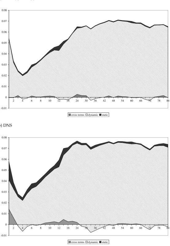
Figure 5 shows the contribution of the static, dynamic and cross terms of Eq. (10) to the totalMSFE(τ) for both the T-FSN(6)-ECM(2) model withk=(1,2,4,18,24,84) and the DNS model (upper and lower panels
Figure 5: MSFE decomposition (a) T-FSN(6)-ECM(2) -0.01 0 0.01 0.02 0.03 0.04 0.05 0.06 0.07 0.08 2 4 6 8 10 12 18 24 30 36 42 48 54 60 66 72 78 84
cross terms dynamic static
(b) DNS -0.01 0 0.01 0.02 0.03 0.04 0.05 0.06 0.07 0.08 2 4 6 8 10 12 18 24 30 36 42 48 54 60 66 72 78 84
cross terms dynamic static
Note: The height at eachτ of a given shaded area is equal to the magnitude of that particular compo-nent ofMSFE(τ). The static component is given byR−1PR
r=1[yOLSr (τ)−yr(τ)]2, the dynamic component by
R−1PR
r=1[ ˆyr|r−1(τ)−yOLSr (τ)]2, and the cross term component by 2R −1PR
r=1[ ˆyr|r−1(τ)−yOLSr (τ)][yOLSr (τ)−yr(τ)] (see Eq. 10).
respectively). The height at each τ of a given shaded area is equal to the magnitude of that particular component (static, dynamic, or cross term). The dynamic component emerges for both models as the largest positive contributor to the totalMSFE(τ) for all maturitiesτ. For all maturities that satisfy 3≤τ≤84, both
the static and dynamic components are positive for DNS and FSN-ECM, and larger for DNS than FSN-ECM. Furthermore, the differences between these components (defined as ‘DNS minus FSN-ECM’) are always larger for the dynamic than the static component, and where the difference in cross terms is negative it is more than offset by the positive difference in the dynamic components. In the case ofτ=1.5 andτ=2, the static component is much larger for DNS than FSN but this difference is more than offset by the dynamic component, the larger MSFE(τ) for DNS then being the result of its large, positive cross term for these maturities.
We conclude that for most maturities, both static and dynamic components contribute to the DNS model having the largerMSFE(τ), but that inferior forecasting of the model-specific, latent factors is more important in this regard. This illustrates a strength of the FSN-ECM framework highlighted previously – namely that a very considerable body of literature exists on how empirically to model economic variables such as log yields using cointegrated VARs. By contrast, the DNS slope and curvature factors are highly specialised to the yield curve context and much less is known about how to specify time series models of factors such as these.
3.6
Parameter estimates for the T-FSN(6)-ECM(2) model
We report here the QMLEs used to produce the constant parameter (C) forecasts of the triangular FSN(6)-ECM(2) model, again withk=(1,2,4,18,24,84). Recall that the MSFEs for constant and recursive estimates in Figure 4(c) are very similar. With the parameters of the ECM state equation (3) set equal to the QMLEs used for the constant parameter forecasts, the knot-yieldsγt follow an I(1) process and the (m−1) spreads
between themβ0sγt are cointegrating relations. This follows since the ranks of ˆαand ˆαβ0sare both equal to five, the rootszof the characteristic polynomial of the VAR in (3) then satisfy eitherz=1 or|z|>1, and the
determinant of [ ˆα0⊥(I−Ψ)βs⊥] is non-zero. The characteristic polynomial of the VAR in (3) thus has exactly
one unit root.
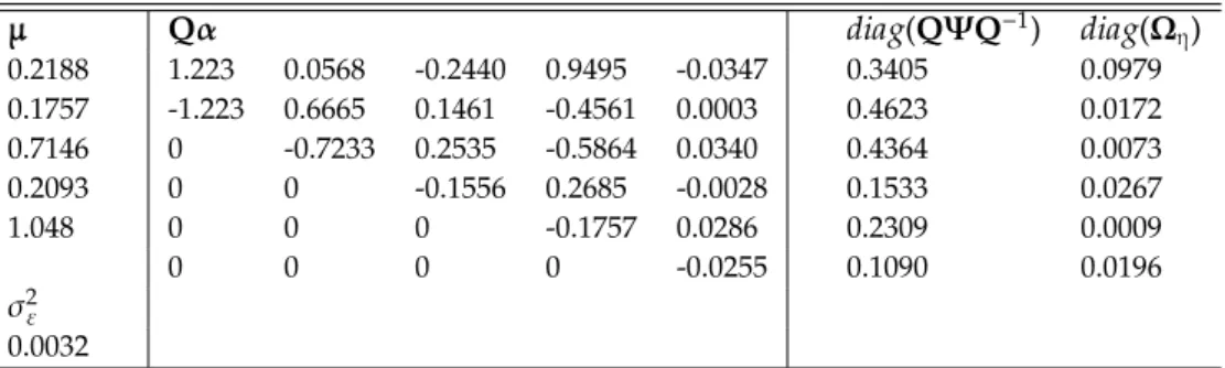
Table 2 reports the QMLEs of the transformed state equation (8), together with ˆσ2ε. Recall that the state vector in (8) isϕt = [γ1t,(β0sγt)0], the vector consisting of the latent short rate and inter-knot yield spreads.
The estimates of the stationary means of the spreadsβ0sγtare all positive, implying that the latent yield curve is ‘upward sloping’ on average. It follows from (8) that
∆γ1,t+1=(Qα)[1](β 0
Table 2: QMLEs of the triangular FSN(6)-ECM(2) model withk=(1,2,4,18,24,84) obtained using the training data from 1985:1 to 2000:12 inclusive as the estimation data
µ Qα diag(QΨQ−1) diag(Ω η) 0.2188 1.223 0.0568 -0.2440 0.9495 -0.0347 0.3405 0.0979 0.1757 -1.223 0.6665 0.1461 -0.4561 0.0003 0.4623 0.0172 0.7146 0 -0.7233 0.2535 -0.5864 0.0340 0.4364 0.0073 0.2093 0 0 -0.1556 0.2685 -0.0028 0.1533 0.0267 1.048 0 0 0 -0.1757 0.0286 0.2309 0.0009 0 0 0 0 -0.0255 0.1090 0.0196 σ2 ε 0.0032
Note:The operationdiag(X) gives the diagonal of the matrixXas a column vector.
where (Qα)[1]denotes the first row of the matrixQα. Bearing in mind thatk=(1,2,4,18,24,84), the estimates
of the row (Qα)[1]in Table 2 are largest in absolute value for the spreads between the first and second, third
and fourth, and fourth and fifth knot-yields. Notice that all elements of the last column ofQαare close to zero, indicating that the spread between the fifth and six knot-yields is unimportant as a regressor in Eq. (8). It also follows from (8) that the vector of spreads follows the VAR
∆(β0sγt+1)=(Qα)[2:6](β0sγt−µ)+(QΨQ−1)[2:6]∆(β0sγt)+η[2:6],t (12)
whereX[2:6]denotes the 2nd to 6th rows of some matrix,X. With parameters set equal to the QMLEs in Table
2, this VAR is stationary. Furthermore, a given spread at (t+1) then dependsonlyon timetspreads involving the same and longer maturities (since (Qα)[2:6]is upper triangular and (QΨQ−1)[2:6]is diagonal) and the same
spread at time (t−1). Note that all elements of the estimate ofQΨQ−1are positive and of the estimate of the
diagonal of (Qα)[2:6]are negative.
4
PROFIT-BASED FORECAST EVALUATION
It is now widely recognised that when comparing forecasting models, each of which may be to some extent mis-specified, no close relationship is guaranteed between model evaluations based on conventional error-based measures such as MSFE and those error-based on the ex post realised pro