1096 DOI: /01.WCB CA

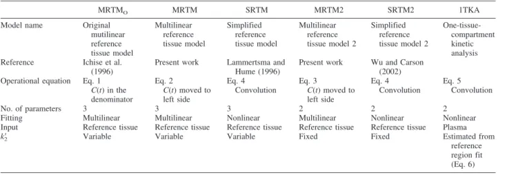
Linearized Reference Tissue Parametric Imaging Methods:

Application to [

11

C]DASB Positron Emission Tomography

Studies of the Serotonin Transporter in Human Brain

*Masanori Ichise, *Jeih-San Liow, *Jian-Qiang Lu, †Akihiro Takano, *Kendra Model,

*Hiroshi Toyama, †Tetsuya Suhara, †Kazutoshi Suzuki, *Robert B. Innis,

and ‡Richard E. Carson

*Molecular Imaging Branch, National Institute of Mental Health, †Brain Imaging Project, National Institute of Radiological Sciences, Chiba, Japan, and ‡PET Department, Warren G. Magnuson Clinical Center, National Institutes of Health,

Bethesda, Maryland, U.S.A.

Summary: The authors developed and applied two new lin-earized reference tissue models for parametric images of bind-ing potential (BP) and relative delivery (R1) for [

11 C]DASB positron emission tomography imaging of serotonin transport-ers in human brain. The original multilinear reference tissue model (MRTMO) was modified (MRTM) and used to estimate a clearance rate (k⬘2) from the cerebellum (reference). Then, the number of parameters was reduced from three (MRTM) to two (MRTM2) by fixingk⬘2. The resultingBPandR1estimates were compared with the corresponding nonlinear reference tissue models, SRTM and SRTM2, and one-tissue kinetic analysis (1TKA), for simulated and actual [11

C]DASB data. MRTM gavek⬘2 estimates with little bias (<1%) and small variability (<6%). MRTM2 was effectively identical to SRTM2 and

1TKA, reducing BP bias markedly over MRTMO from 12– 70% to 1–4% at the expense of somewhat increased variability. MRTM2 substantially reducedBPvariability by a factor of two or three over MRTM or SRTM. MRTM2, SRTM2, and 1TKA hadR1bias <0.3% and variability at least a factor of two lower than MRTM or SRTM. MRTM2 allowed rapid generation of parametric images with the noise reductions consistent with the simulations. Rapid parametric imaging by MRTM2 should be a useful method for human [11

C]DASB positron emission to-mography studies. Key Words: Positron emission tomogra-phy—Parametric imaging—Linearized reference tissue model—Noise-induced bias—Serotonin transporters— [11

C]DASB.

The central serotonergic (5-HT) system has been linked to the pathophysiology and drug treatment of neu-ropsychiatric conditions such as depression and obses-sive compulobses-sive disorder (Lopez-Ibor, 1988). The sero-tonin transporter (SERT) is a critical modulator of 5-HT neurotransmission and the site of action of commonly used antidepressant drugs (Lesch, 1997). Therefore, in vivoimaging of the SERT has been of intense interest as a tool to study 5-HT function in health and disease. A recently developed highly selective radioligand, [11

C]-3- amino-4-(2-dimethylaminomethyl-phenylsulfanyl)-benzonitrile ([11C]DASB), is most promising for posi-tron emission tomography (PET) imaging of SERT in human brain (Ginovart et al., 2001; Houle et al., 2000; Huang et al., 2002; Wilson et al., 2000a). [11C]DASB binds reversibly to SERT with high affinity and selec-tivity (Wilson et al., 2000a, 2002), and displays moder-ately high specific-to-nonspecific ratiosin vivo(Ginovart et al., 2001; Houle et al., 2000). [11C]DASB tissue data can be described by a one-tissue (1T) compartment model (Ginovart et al., 2001) and SERT binding poten-tial (BP; Mintun et al., 1984) can be estimated using the cerebellum, which contains few SERT binding sites, as reference tissue instead of an arterial input function. The regional distribution of BP correlates well with SERT densities in human brain (Ginovart et al., 2001; Houle et al., 2000).

Reference tissue methods have been widely used to estimate neuroreceptor BP because these methods Received February 14, 2003; final version received June 12, 2003;

accepted June 16, 2003.

Supported by the Neuroscience project of the National Institute of Radiological Sciences, Chiba, Japan, and Japan Society for the Promo-tion of Science, Grant-in-Aid for Scientific Research 14370296, Tokyo, Japan.

Address correspondence and reprint requests to Dr. Ichise, Building 1 B3–10, One Center Drive MSC0135, Molecular Imaging Branch, National Institute of Mental Health, Bethesda, MD 20892, U.S.A.; e-mail: [email protected]

eliminate the invasive and often logistically difficult pro-cedure of obtaining arterial input functions corrected for metabolites. For [11C]DASB, reference tissue meth-ods that yield parametric images ofBPwould be a valu-able data analysis approach because SERT binding sites are widely distributed in the brain, including small limbic structures such as the raphe, hippocampus, and amygdala (Backstrom et al., 1989; Cortes et al, 1988; Rosel et al., 1997).

For reversibly binding neuroreceptor radioligands, several reference tissue models have been developed to estimate BP (Ichise et al., 1996; Lammertsma et al., 1996; Lammertsma and Hume, 1996; Logan et al., 1996) as well as a measure of radioligand delivery to tissue relative to reference region (R1) (Lammertsma et al., 1996; Lammertsma and Hume, 1996). These models are generally an extension of either traditional compartmen-tal kinetic models (Lammertsma et al., 1996; Lam-mertsma and Hume, 1996) or their linearized versions (Ichise et al., 1996; Logan et al., 1996). The computa-tionally rapid linear least squares (LS) estimation algo-rithms used in the latter approach is well suited for rapid parametric imaging compared with the more computa-tionally time-consuming nonlinear least squares (NLS) algorithms used in the former, although basis function methods can be used to improve NLS processing speed (Gunn et al., 1997). One drawback of the linear LS ap-proach as originally described, however, is that statistical noise, particularly at the voxel level in the PET data, can introduce significantly bias in the parameter estimates (Carson, 1993; Slifstein and Laruelle, 2000). Subse-quently, several strategies have been proposed to reduce noise-induced bias for LS parameter estimation (Carson, 1993; Ichise et al., 2002; Logan et al., 2001; Varga et al., 2002).

Here, we developed two new linearized reference tis-sue models that are resistant to noise, computationally fast, and do not require invasive blood sampling. These models were used to generate parametric images ofBP

and R1 for [ 11

C]DASB PET data. To reduce noise ef-fects, we applied two strategies to the multilinear refer-ence tissue model (Ichise et al., 1996). First, the multi-linear operational equation, which estimates three parameters includingBPandk⬘2(the clearance rate con-stant from the reference region), was rearranged to re-move a noisy tissue radioactivity term, C(T), from the independent variables, following the strategy known to be effective in reducing the noise-induced bias for the LS models requiring blood data (Carson, 1993; Ichise et al., 2002). Second, the number of parameters in this newly rearranged multilinear reference tissue model (MRTM) was reduced from three to two, by fixing k⬘2to a value estimated by preliminary application of MRTM for se-lected regions of interest (ROIs), following the strategy also known to be effective in noise reduction for the NLS

simplified reference tissue model (SRTM) (Wu and Car-son, 2002). The parameter estimation results for this new two-parameter model (MRTM2) from simulated and ac-tual [11C]DASB data were compared with the other es-timation methods, particularly the two-parameter SRTM (SRTM2) and the one-tissue kinetic analysis (1TKA) that requires blood data, with the hypothesis that MRTM2 will produce results comparable with SRTM2 and 1TKA If this is the case, then MRTM2 should be a highly useful data analysis tool for [11C]DASB because parametric imaging with MRTM2 can be performed in a fraction of the computational time required for SRTM2 or 1TKA.

MATERIALS AND METHODS Theory

Multilinear reference tissue models.The operational equa-tion for the original multilinear reference tissue model (MRTMO, Ichise et al., 1996) is as follows:

兰

兰

−1

) is the clearance rate constant from the reference region to plasma, and b is the intercept term, which becomes constant forT>t*. Eq. 1 allows estimation of three parameters,␤1⳱V/V⬘,␤2⳱V/(V⬘k⬘2), and

␤3⳱bby multilinear regression analysis forT>t*. Note that Eq. 1 and all subsequent linear equations are applicable to both 1T and two-tissue (2T) compartment models. Assuming that the nondisplaceable distribution volumes in the tissue and ref-erence regions are identical,BP(BP⳱V/V⬘− 1) is calculated from the first regression coefficient asBP ⳱ (␤1 − 1). For radioligands with 1T kinetics such as [11

C]DASB (Ginovart et al., 2001), Eq. 1 is linear fromT⳱0, i.e.,t*⳱0, andbis equal to (−1/k2), wherek2(min

−1

) is the clearance rate constant from the tissue to plasma. For the 1T model,V⳱K1/k2andV⬘

⳱K⬘1/k⬘2, whereK1andK⬘1(mL/min −1

/mL−1) are the rate con-stants for transfer from plasma to the tissue and reference re-gion, respectively, andR1 ⳱ K1/K⬘1, the relative radioligand delivery, can be calculated from the ratio of the second and third regression coefficients asR1⳱−␤2/␤3.

Ordinary LS parameter estimation assumes that independent variables are noise-free. However, Eq. 1 contains a noisy term, C(T), on the right-hand side (independent variables). In addi-tion, the structure of Eq. 1 makes noise in the dependent (left-hand side) and independent variables correlated. These factors produce biased estimates (Carson, 1993; Ichise et al., 2002; Slifstein and Laruelle, 2000). Following the strategy described previously to reduce noise-induced bias for linear estimation of Vusing tissue and blood data (Ichise et al., 2002), Eq. 1 can be rearranged to yield the following multilinear reference tissue model (MRTM): C共T兲= − V V⬘b

兰

兰

In Eq. 2, noisyC(T) is no longer present in the independent variables, although integral ofC(t) is present. However, inte-grals of noisy data typically have much lower percent variation than the data themselves (Ichise et al., 2002). Additionally, the correlation of the noise in the dependent and independent vari-able is dramatically reduced in Eq. 2 compared with Eq. 1. Eq. 2 also allows estimation of three parameters,␥1⳱−V/(V⬘b),␥2

⳱1/band␥3⳱−V/(V⬘k⬘2b), assuming that the integrals ofC(t) and C⬘(t), as well as C⬘(T), are noise-free. BP can then be calculated from the ratio of the two regression coefficients as BP⳱−(␥1/␥2+ 1). For the 1T modelR1⳱␥3andk2⳱−␥2. Eq. 2 also allows estimation ofk⬘2, which is given byk⬘2⳱

␥1/␥3. However, a different value ofk⬘2is estimated by Eq. 2 for each voxel, although there is only one reference region and therefore only one true value fork⬘2. By fixingk⬘2 to a value obtained with a preliminary analysis using Eq. 2, a two-parameter version of Eq. 2 (MRTM2) is obtained by rearrange-ment to yield C共T兲= − V V⬘b

冉

兰

冊

兰

Eq. 3 can also be obtained by rearrangement of the graphical reference tissue model described by Logan et al. (1996). Eq. 3 estimates two parameters,␥1⳱−V/(V⬘b) and␥2⳱1/bforT >t*, assuming that the integrals ofC(t) andC⬘(t), as well as C⬘(T), are noise-free.BPis then calculated from the ratio of the two regression coefficients asBP⳱− (␥1/␥2+ 1). For the 1T model,R1⳱␥1/k2⬘andk2⳱−␥2. Because MRTM2 estimates fewer parameters, it is expected to be more stable than MRTM, particularly at high-noise levels of voxel-based parametric im-aging. This strategy has been shown to be effective in reducing noise from the three-parameter simplified reference tissue model (SRTM) to the two-parameter model SRTM2 (Wu and Carson, 2002).

Simplified reference tissue models

The operational equation for the SRTM (Lammertsma and Hume, 1996) is

C共t兲=R₁C⬘共t兲+R₁共k⬘₂−k₂兲C⬘共t兲丢e−k2t

(4) where丢is the convolution symbol. Note that Eq. 4 is derived from the 1T compartment model unlike the above linear equa-tions that are applicable to both 1T and 2T compartment mod-els. Eq. 4 allows NLS estimation of three parameters from the entire data set,R1,k⬘2, andk2.BPis calculated from the rela-tionship,BP ⳱ R1(k⬘2/k2) − 1. In the two-parameter SRTM2 method (Wu and Carson, 2002), the value ofk⬘2is fixed so that Eq. 4 estimates two parameters,R1andk2.

One-tissue compartment kinetic analysis.The operational equation for 1TKA is

C共t兲=K1CP共t兲丢e −k2t

(5) whereCP(t) is the metabolite-corrected plasma concentration (kBq/mL). Eq. 5 allows NLS estimation of two parameters from the entire data set,K1and k2.BPand R1are calculated from the relationship,BP⳱(K1k⬘2/K⬘1k2) − 1 andR1⳱K1/K⬘1, whereK⬘1 and k⬘2 are estimated by 1TKA applied to the ref-erence region time–activity curve (TAC), with the follow-ing equation:

C⬘共t兲=K⬘₁C_P共t兲丢e−k₂⬘t

(6)

Positron emission tomography studies [11

C]DASB PET studies were performed in eight normal control subjects (mean age, 21.8 ± 2.4 years; age range, 20–27 years). The study protocol was approved by the ethics and radiation safety committees of the National Institute of Radio-logical Sciences (Chiba, Japan), and written informed consent was obtained from each subject. [11

C]DASB was synthesized as described previously (Wilson et al., 2000a,b). After a 10-minute transmission scan using a68

Ge-68

Ga source, dynamic PET scans were acquired for 90 minutes (27 frames consisting of 4 × 1, 13 × 2, 5 × 4 and 5 × 8-minute frames) after bolus administration of 630 ± 51 MBq (specific activity, 70–196 GBq/␮mol at the time of injection) of [11

C]DASB on the ECAT 47 (CTI-Siemens, Knoxville, TN, U.S.A.) scanner in two-dimensional mode, which provides 47 slices with 3.38-mm center-to-center slice separation. To minimize head movement during each scan, head fixation devices (Fixster Instruments, Stockholm, Sweden) and thermoplastic attachments made to fit the individual subject were used. The PET data were recon-structed using a Hann filter with a cut-off frequency of 0.5 resulting in image full width at half maximum of 9.3 mm.

Arterial blood samples were taken 13 times during the initial 3 minutes after the tracer injection, then eight times during the next 17 minutes, and then once every 10 minutes until the end of the scan. Each blood sample was separated into plasma and blood cell fraction by centrifugation. For the plasma fractions at 3.5, 9, 19, 29, 39, 49, 59, 69, 79, and 89 minutes after injection, acetonitrile was added and the sample was centrifuged. The obtained supernatant was subjected to radio-HPLC analysis (column ␮Bondapak C18; mobile phase, phosphoric acid [6 mmol/L]/CH3CN⳱1:1; flow rate, 2.5 mL/min). The fraction of unchanged radioligand in plasma was fitted to a sum of two exponentials. A metabolite-corrected plasma curve was gener-ated by the product of the plasma activity and metabolite frac-tion curves. The porfrac-tion of the metabolite-corrected plasma curve beyond the initial peak was fit to a sum of two exponen-tials (three exponenexponen-tials did not improve fitting). The resulting curve was used as the input function for estimation of 1T ki-netic parameter values (see below). Plasma protein binding was not determined in the present study.

Simulation analysis

Table 1 lists the characteristics of the six models used for the simulation analysis and the analysis of human PET data. For the simulation, bias and variability ofBPandR1estimates by all six models due to statistical noise were evaluated with simu-lated [11

C]DASB TACs at different noise levels. Gray matter regions with a range of BP (raphe, striatum, thalamus, and frontal cortex) were simulated. Even thoughBPmeasurement in white matter may not be of biological interest, simulations in white matter with very lowBPwere also performed because poor estimation characteristics there would contribute to arti-facts in parametric images.

In addition, the feasibility of obtaining a stablek⬘2value to be used for MRTM2 and SRTM2 was evaluated by application of MRTM to ROI TACs. To this end, bias and variability ofk⬘2 estimates by MRTM were calculated for simulated [11

C]DASB TACs at different ROI noise levels. The variability ofBPand R1 estimates from simulation were, when appropriate, com-pared with the respective theoretical variability, as predicted by the Cramer-Rao (C-R) lower bounds for the two-parameter and three-parameter models (Beck and Arnold, 1977; Wu and Car-son, 2002).

To perform [11

C]DASB TAC simulations, a metabolite-corrected plasma input function that had a typical clearance (175 L/h) was selected from a normal control study, and was

scaled to a group mean injection dose of 630 MBq. TACs were simulated using the 1T parameter values (Table 2). Intravascu-lar radioactivity was not included because its contribution would be minimal owing to the highK1andVvalues. These parameter values were derived from the group meanK⬘1,K1,V⬘, and Vvalues estimated by 1T KA for the respective regions (see below).

Noise-free TACs were generated for 90 minutes (54 frames of 30-second to 4-minute duration with TAC values calculated at the midframe time). The sampling rates used in the simula-tions were twice the rates used in actual PET studies to mini-mize any bias introduced by the integral(s) on the right-hand side of the operational equations. Then, random amounts of normally distributed mean zero noise were added to the noise-free TAC with SD according to the following formula:

SD共ti兲=SF

冉

␭ti_C共ti兲 ⌬ti

冊

0.5

(7) whereSF is the scale factor that controls the level of noise; C(ti) is the noise-free simulated radioactivity;⌬tiis the scan duration (seconds); and␭ is the radioisotope decay constant. This model is appropriate in the case of low or constant ran-doms fractions, constant scatter fraction, and relatively un-changing emission distribution over time. One thousand noisy TACs were generated for several values of SF so that TAC noise levels ranged from 5 to 30%. Percent TAC noise was calculated from the mean SD (Eq. 7) of the latter portion of the TAC (50 to 90 minutes). These noise levels would cover a range of TAC noise between that found in a small ROI to that of a voxel.

The noise-free reference tissue TAC for all reference tissue models and the truek⬘2value of 0.056 min

−1

for MRTM2 and SRTM2 were used in fitting noisy tissue TACs (see Discus-sion). Equal data weights were used for all methods (see Dis-cussion). Because all TACs were simulated consistent with the 1T model,t* was set to 0 for MRTMO, MRTM, and MRTM2. The first time point was excluded from fitting, however, to minimize any bias introduced by the integral(s) on the right-hand sides of the operational equations. For SRTM, SRTM2, and 1TKA, the initial parameter values were chosen randomly from the range of 75 to 125% of the true parameter value. To calculateBP andR1 for 1TKA, the true values ofK⬘1and k⬘2 were used for consistency with the use of noise-freeC⬘(t) in the reference tissue methods. Parameter estimates were considered outliers ifBPorR1values were less than zero or more than five

times the true values, which should include nonconvergence cases. Bias was expressed as percent deviation of the sample mean from the true value and the variability was calculated as percent sample SD relative to the true value excluding outliers. Theoretical BP and R1variability were calculated as percent C-R SD relative to the true value.

For MRTM2 and SRTM2,k⬘2will be estimated by prelimi-nary application of MRTM or SRTM to ROI TACs. To assess the magnitude of noise in this ROI-basedk⬘2estimation, 1,000 noisy tissue TACs were generated at noise levels ranging from 1 to 7%, which would cover a range of TAC noise found in large to small ROIs.k⬘2was estimated by MRTM, with sample bias and sample variability ofk⬘2calculated as above. In addi-tion, the effect of error ink⬘2estimates on MRTM2 estimation ofBPandR1was evaluated by calculating the bias ofBPand

R1 estimates by fitting the original gray matter TACs using biased k⬘2 values (ranging from −6 to +6%). All simulation analyses were performed in MATLAB (The MathWorks, Natick, MA, U.S.A.), or pixel-wise kinetic modeling (PMOD) software (PMOD Group, Zurich, Switzerland).

Positron emission tomography study analysis The original reconstructed PET data were corrected for sub-ject motion by registering each frame to a summed image of all frames, and the summed PET image was coregistered to a T1-weighted magnetic resonance image (repetition time/echo time⳱21/9.2 milliseconds), acquired on a 1.5-T Phillips In-tera (Phillips Medical Systems, Best, The Netherlands), in both cases using a six-parameter mutual information registration technique (Jenkinson et al., 2002) in the image analysis soft-ware MEDx (Sensor Systems Inc., Sterling, Virginia, U.S.A). TABLE 1. Model summary

MRTMO MRTM SRTM MRTM2 SRTM2 1TKA

Model name Original

mutilinear reference tissue model Multilinear reference tissue model Simplified reference tissue model Multilinear reference tissue model 2 Simplified reference tissue model 2 One-tissue-compartment kinetic analysis

Reference Ichise et al.

(1996)

Present work Lammertsma and Hume (1996)

Present work Wu and Carson (2002) Operational equation Eq. 1

C(t) in the denominator Eq. 2 C(t) moved to left side Eq. 4 Convolution Eq. 3 C(t) moved to left side Eq. 4 Convolution Eq. 5 Convolution No. of parameters 3 3 3 2 2 2

Fitting Multilinear Multilinear Nonlinear Multilinear Nonlinear Nonlinear

Input Reference tissue Reference tissue Reference tissue Reference tissue Reference tissue Plasma

k⬘2 Variable Variable Variable Fixed Fixed Estimated from

reference region fit (Eq. 6)

TABLE 2. One-tissue-compartment kinetic parameter values used for simulating time–activity curves

Region K₁ (mL⭈min−1_⭈mL−1₎ k₂ (min−1_{) BP R} 1 Cerebellum* 0.615 0.056 — — Raphe 0.496 0.013 2.55 0.81 Striatum 0.656 0.023 1.64 1.07 Thalamus 0.662 0.021 1.91 1.08 Frontal cortex 0.697 0.050 0.27 1.13 White matter 0.260 0.022 0.09 0.42

* TheK₁ andk₂ values for cerebellum (reference region) refer to those ofK⬘1andk⬘2, respectively.

The summed PET image was then fused with the coregistered magnetic resonance image using an image fusion tool in PMOD. Several anatomical ROIs were manually defined on this fused image, and ROI TACs from the cerebellum (∼400 voxels, voxel size⳱3.4 × 3.4 × 3.4 mm), raphe (∼40 voxels), striatum (∼110 voxels), thalamus (∼90 voxels), frontal cortex (∼400 voxels), and white matter (∼200 voxels) were obtained. These ROI TACs were fitted by 1TKA using individual me-tabolite-corrected plasma input functions. The mean 1TKA pa-rameter values from five of eight subjects were used to generate noise-free TAC data, as described in the previous section re-garding simulation analysis.

To compare voxel-wise BP and R1 estimates between the different reference tissue models as well as 1TKA, individual-voxel TACs were obtained from the raphe, striatum, and frontal cortex. MRTM2 and SRTM2 require a priori knowledge of value, which was provided by preliminary application of MRTM. To minimize the variability of estimation by MRTM (see the simulation results), a weighted (according to ROI size) mean value estimated from ROI TACs of raphe, striatum, and thalamus was used. To calculate BP and R1 for 1TKA, the values ofk⬘2andK⬘1estimated by 1TKA for the cerebellar ROI were used. Parameter estimate outliers were arbitrarily defined asBPorR1values less than zero or more than five times the same values used in the simulation analysis.

For comparison to simulations, percent ROI and voxel TAC noise was calculated based on deviations from 1TKA fitting for the latter portion of the TAC (50 to 90 minutes). ROI noise values [mean ± SD (range)] were 3.1 ± 1.0% (2.1–4.9%), 1.9 ± 0.5% (1.1–2.3%), 2.4 ± 0.6% (1.2–2.8%) and 2.6 ± 0.6% (1.8– 3.1%) in the raphe, striatum, thalamus, and frontal cortex, re-spectively. Voxel noise values were 12 ± 4%, 11 ± 4%, 15 ± 5%, and 23 ± 8% in the raphe, striatum, frontal cortex, and white matter, respectively. If the actual scan data had been acquired with the doubled sampling rate, as used in the simu-lation, all these noise values would have increased by a factor of √2. Thus, for comparison to the simulations, the percent noise values in the actual PET data were multiplied by √2. Thus, ROI noise values of 3 to 7%, 2 to 3%, 2 to 4%, and 2 to 4% in the raphe, striatum, thalamus, and frontal cortex, respec-tively, and voxel noise values of 15% and 30% for gray and white matter, respectively, were chosen as typical noise levels in evaluating the simulation results.

Comparison of estimates between MRTM and 1TKA as well as comparison of voxel-basedBPandR1estimates between all methods were made by performing paired t-tests. Statistical significance was defined asP< 0.05.

Parametric images of BPand R1were generated from the motion-corrected data sets (n ⳱ 8) by MRTMO(BP only), MRTM2, SRTM2, and SRTM, respectively. The SRTM and SRTM2 parametric imaging was performed based on the basis function method of Gunn et al. (1997) to improve processing speed. All parametric imaging was performed in PMOD in-stalled on a PC workstation (Dell Computer Co., Austin, TX, U.S.A., 1.7 GHz Pentium IV/1 GB-RAM running Microsoft Windows 2000, Microsoft Co., Redmond WA, U.S.A). PMOD is platform-independent software programmed in Java environ-ment (Mikolajczyk et al., 1998).

RESULTS Simulation analysis

[11C]DASB time–activity curves. The cerebellum TAC and frontal cortex TAC with a lowBP(0.27) had the earliest peaks (Fig. 1A), whereas the striatum (1.64),

thalamus (1.91), and raphe (2.55) TACs peaked later. The white matter TAC with a very low BP (0.09) in-creased slowly, peaked late, and reached the level of the cerebellum or frontal cortex by 75 to 90 minutes. Even with high radioligand delivery (Table 2), the [11C]DASB TACs were slow to reach their peaks because of the relatively high distribution volumes. The noisy striatal TACs (Fig. 1B) showed considerably more variability at later time points, as produced by Eq. 7.

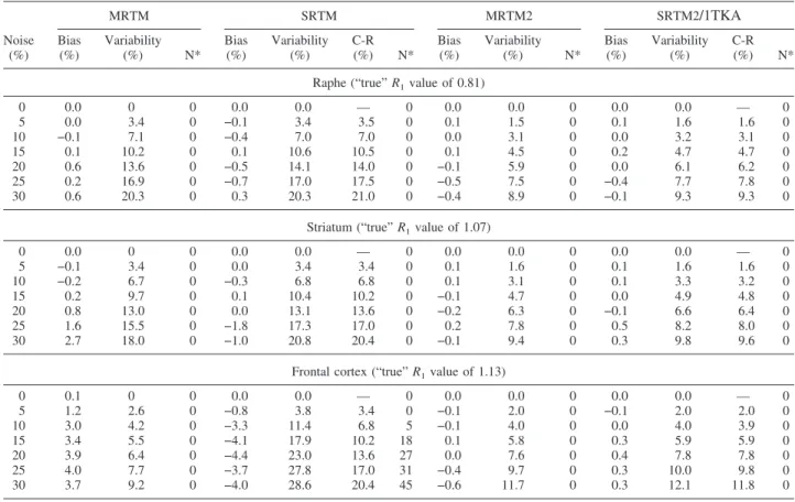
BP estimation. Table 3 shows BP percent bias and variability by all methods for simulated data at different noise levels in the raphe, striatum, and frontal cortex,

FIG. 1. Simulated [11_{C]DASB noise-free time–activity curves (A)}

and examples of noise-added time–activity curves for the stria-tum at noise levels 0%, 15%, and 30% (B).

and Fig. 2 depicts the bias (Fig. 2A) and variability (Fig. 2B) for the three gray matter regions together at the typical gray matter noise level of 15%. The three-parameter methods, MRTM and SRTM, had very similar characteristics. The two-parameter versions, MRTM2 and SRTM2, were also similar. SRTM2 and the two-parameter 1TKA produced identical two-parameter estimates to three significant digits (Table 3; see Discussion). MRTM2, SRTM2, and 1TKA all had the smallest mag-nitude of bias due to noise (1–4%, Fig. 2A). The vari-ability for these three methods (12–20%, Fig. 2B), how-ever, was somewhat higher than that of MRTMObut was substantially lower than that of MRTM or SRTM. Note that the two-parameter methods had the advantage over the other three-parameter methods of exact knowledge of the k⬘2 value. Regionally, the percent variability for the two-parameter methods was larger in the high-BPraphe and the low-BP frontal cortex, and somewhat lower in the intermediate-BP striatum. These sample variability values showed good agreement with the predicted C-R values (Table 3), except at the highest noise levels in the

raphe. There were no outliers for the two-parameter methods except for a few at the highest noise levels (Table 3). Overall, BP estimates by MRTM2 and SRTM2 were effectively identical, with mean

percent-BPdifferences between the two models over 1,000 runs at 15% noise of 0 ± 1%, 0 ± 1%, and 1 ± 6% for raphe, striatum, and frontal cortex, respectively.

MRTMO had the largest magnitude of bias (−12 to −70%, Fig. 2A), but the smallest variability (4–14%, Fig 2B), and no outliers except at the highest noise level (Table 3). MRTM and SRTM, had magnitudes of bias intermediate between MRTMOand MRTM2, SRTM2, or 1TKA (∼20%, Fig. 2A), the largest variability (40–70%, Fig. 2B), and large numbers of outliers up to 10% at 15% noise (Table 3). Unlike MRTM2, SRTM2, or 1TKA, the variability values for MRTM and SRTM showed a no-ticeable discrepancy from the C-R values, even at mod-erate noise levels (see Discussion). However, this dis-crepancy artifactually appeared to decrease with increasing number of outliers because the variability val-ues were calculated excluding the outliers (Table 3). The

TABLE 3. Bias and variability of binding potential (BP) estimates by six different models for simulated [11

C]DASB data at different noise levels

Noise (%) MRTM_O MRTM SRTM MRTM2 SRTM2/1TKA Bias (%) Variability (%) N* Bias (%) Variability (%) N* Bias (%) Variability (%) C-R (%) N* Bias (%) Variability (%) N* Bias (%) Variability (%) C-R (%) N*

Raphe (“true”BPvalue of 2.55)

0 0.0 0 0 −0.1 0 0 −0.1 0 — 0 −0.1 0 0 0.0 0 — 0 5 −55.4 7.5 0 5.2 20.3 0 5.1 20.4 15.5 0 0.6 5.9 0 0.7 6.0 5.9 0 10 −66.7 3.5 0 15.8 52.1 29 15.3 52.5 31.1 28 1.6 12.0 0 1.6 12.3 11.7 0 15 −69.4 2.9 0 21.4 70.9 83 20.7 72.0 46.6 79 3.6 20.1 0 3.6 20.5 17.6 0 20 −70.5 3.1 0 17.7 75.3 158 15.6 74.5 62.1 153 4.8 27.5 0 4.7 28.0 23.5 0 25 −71.6 3.7 0 16.6 79.5 238 14.6 81.5 77.7 227 9.9 40.4 1 9.7 40.9 29.3 1 30 −72.5 4.7 0 9.9 78.2 278 6.2 78.1 93.2 263 14.1 51.4 6 13.7 51.7 35.2 6

Striatum (“true”BPvalue of 1.64)

0 −0.1 0 0 −0.1 0 0 0.0 0 — 0 −0.1 0 0 0.0 0 — 0 5 −32.6 6.0 0 2.7 11.1 0 2.6 11.1 9.4 0 0.3 3.9 0 0.3 4.0 4.0 0 10 −42.1 3.5 0 10.7 37.8 15 10.0 38.4 18.8 14 0.7 7.9 0 0.7 8.0 7.9 0 15 −44.5 3.7 0 14.8 47.3 56 13.7 49.9 28.3 51 1.0 11.8 0 0.9 12.0 11.9 0 20 −45.6 4.5 0 17.8 63.7 105 13.7 60.4 37.7 101 1.7 16.8 0 1.5 17.2 15.8 0 25 −46.6 5.4 0 18.6 68.0 172 13.2 65.0 47.1 161 4.8 22.8 0 4.6 23.4 19.8 0 30 −47.3 6.6 0 13.4 74.5 184 5.3 68.4 56.5 166 6.3 27.1 0 5.8 27.5 23.7 0

Frontal cortex (“true”BPvalue of 0.27)

0 −0.1 0.0 0 −0.1 0 0 0.0 0 — 0 −0.1 0.0 0 0.0 0 — 0 5 −11.4 4.7 0 11.6 41.3 42 6.7 35.6 12.8 31 0.1 6.9 0 0.1 6.8 6.8 0 10 −11.8 8.7 0 11.3 61.7 100 3.3 51.8 25.7 61 1.2 14.1 0 1.0 14.1 13.5 0 15 −11.9 13.5 0 2.1 59.0 106 −4.5 39.6 38.5 48 1.4 20.7 0 1.0 20.4 20.3 0 20 −12.1 18.0 0 6.5 71.1 113 −5.2 41.9 51.4 49 2.6 27.8 0 1.9 27.4 27.0 0 25 −12.3 22.4 0 5.5 68.3 144 −4.3 48.5 64.2 46 4.1 35.1 0 3.0 34.6 33.8 0 30 −12.6 26.8 2 10.7 79.0 162 −5.4 44.2 77.1 57 6.5 42.1 4 4.6 41.8 40.5 2

Bias and variability are expressed as mean percent deviation ofBPfrom the true value and percent SD of sample excluding outliers (nⱕ1,000) relative to the trueBPvalue, respectively. SRTM2 and 1TKA have identical estimation characteristics in this simulation.

* N indicates the number of outliers.

C-R, theoretical variability values ofBPestimates as predicted by the Cramer-Rao lower bound; MRTMO, MRTM, MRTM2, original multilinear reference tissue model, its rearranged three-parameter model and two parameter model, respectively; SRTM, SRTM2, simplified reference tissue model and its two-parameter model, respectively; 1TKA, one-tissue kinetic analysis.

bias and variability were similar for MRTM and SRTM in both the striatum and raphe. However, in the frontal cortex, MRTM had somewhat larger variability than SRTM, with more outliers at all noise levels (Table 3). Thus, MRTM2, SRTM2 and 1TKA, given knowledge of k⬘2 all markedly reduced the magnitude of BP bias compared with MRTMO at the expense of somewhat increased variability. Furthermore, these methods con-siderably reducedBPbias in the high-BPregions andBP

variability in all regions by a factor of two or three com-pared with MRTM or SRTM (Table 3).

For the white matter, however, BP estimation tended to be unstable for all methods, particularly for MRTMO, MRTM, and SRTM. For example, at the typical white matter noise level, BP estimates were all negative for MRTMO, whereas the mean ± SD (range) values ofBP estimates over 1,000 runs for SRTM, MRTM2, and SRTM2/1TKA were −0.10 ± 6.48 (−168 to +93), 0.14 ± 0.22 (−0.29 to +2.08), and 0.13 ± 0.23 (−0.30 to +2.08),

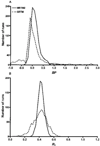
respectively. This instability of BP estimation in the white matter suggested that parametric images from these latter methods will contain some white matter vox-els with inappropriately high positive BP values, due simply to statistical noise in the data. For example, his-tograms of BP estimates for MRTM2 and SRTM are shown in Fig. 3A, where 1% and 5% of voxels hadBP

values >1, respectively. Although the BP in the white matter is not generally of pathophysiologic interest, para-metric images with noisy white matter voxels could be visually misleading.

R1estimation.Table 4 shows the bias and variability

of R1 estimates at different noise levels in the raphe, striatum, and frontal cortex, and Fig. 4 depicts the bias (Fig. 4A) and variability (Fig. 4B) for the gray matter regions at 15% noise. MRTM2, SRTM2, and 1TKA all had the smallest magnitudes of bias (<0.3% for all noise levels and gray matter regions), as well as the smallest variability (<6%, Fig. 4B), at least a factor of 2 lower than SRTM, and no outliers (Table 4). The variability values were in close agreement with the C-R bounds. TheseR1bias and variability values were considerably

FIG. 2. Bias (A) and variability (B) ofBPestimates by six differ-ent models using simulated [11_{C]DASB time–activity curves for}

raphe, striatum, and frontal cortex at 15% noise. SRTM2 and 1TKA have identical estimation characteristics in this simulation. MRTMO, MRTM, and MRTM2 indicate original multilinear

refer-ence tissue model, its rearranged three-parameter model and two-parameter model, respectively;BP, binding potential; SRTM and SRTM2, simplified reference tissue model and its two-parameter model, respectively; 1TKA, one-tissue compartment kinetic analysis.

FIG. 3. Histograms of estimatedBP(A) andR1(B) by MRTM2

and SRTM for simulated white matter time–activity curves at 30% noise (1,000 runs).BP, binding potential;R1, relative delivery;

MRTM2, two-parameter multilinear reference tissue model; SRTM, simplified reference tissue model.

smaller than the corresponding values forBPestimations (Table 3). As was the case forBPestimates,R1estimates by MRTM2 and SRTM2 were virtually identical, with percent differences between the two models over 1,000 runs of 0.1 ± 0.4%, −0.1 ± 0.6%, and 0.4 ± 1.0% for raphe, striatum, and frontal cortex, respectively; andR1 estimates by SRTM2 and 1TKA were identical to three significant digits (see Discussion).

Both MRTM and SRTM had slightly larger magni-tudes of bias (up to 4%, Fig. 4A) and higher variability by a factor of two or three (Fig. 4B) than did MRTM2, SRTM2, or 1TKA, except that MRTM had variability in the frontal cortex comparable with that for MRTM2, SRTM2, or 1TKA (see Discussion). However, MRTMO

R1estimation (data not shown) was very unstable, with outliers exceeding 50% at 15% noise and beyond for all gray matter regions.

Finally, for the white matter, unlikeBPestimates,R1 estimates by MRTM, SRTM, MRTM2, SRTM2 and 1TKA were stable with no outliers, as shown in the his-togram for SRTM and MRTM2 in Fig. 3B.

Fig. 5 shows the correlation scatterplot between the MRTM2 parameter estimates␥1and␥2from the 1,000 simulated realizations in the three gray matter regions and white matter. For convenience of scale and interpre-tation, the parameters have been divided byk⬘2so the x and y axes are R1 andk2/k⬘2, respectively. For a given region, the parameter estimates are correlated; this is reflected in the nonzero slope of the elliptical cloud of parameter estimates. For example, for voxels with lower than averageR1, the estimatedk2also tended to be lower than the mean, resulting in increased values ofBP. For white matter values, the spread of voxel noise produces a wide range ofBPvalues with a long positive tail (Fig. 3A). The correlation plot in Fig. 5 suggested that appro-priate thresholds using estimatedR1andBPvalues might lead to an algorithm that would eliminate the potentially misleading voxels in white matter with highBP values produced by noise. For example, the simplest approach would be to assign aBPvalue of zero to all voxels with

R1values below a certain cutoff value, which might re-sult in cosmetically more satisfactory parametric BP

TABLE 4. Bias and variability of relative delivery (R1) estimates by five different models for simulated [ 11

C]DASB data at different noise levels

Noise (%) MRTM SRTM MRTM2 SRTM2/1TKA Bias (%) Variability (%) N* Bias (%) Variability (%) C-R (%) N* Bias (%) Variability (%) N* Bias (%) Variability (%) C-R (%) N*

Raphe (“true”R₁value of 0.81)

0 0.0 0 0 0.0 0.0 — 0 0.0 0.0 0 0.0 0.0 — 0 5 0.0 3.4 0 −0.1 3.4 3.5 0 0.1 1.5 0 0.1 1.6 1.6 0 10 −0.1 7.1 0 −0.4 7.0 7.0 0 0.0 3.1 0 0.0 3.2 3.1 0 15 0.1 10.2 0 0.1 10.6 10.5 0 0.1 4.5 0 0.2 4.7 4.7 0 20 0.6 13.6 0 −0.5 14.1 14.0 0 −0.1 5.9 0 0.0 6.1 6.2 0 25 0.2 16.9 0 −0.7 17.0 17.5 0 −0.5 7.5 0 −0.4 7.7 7.8 0 30 0.6 20.3 0 0.3 20.3 21.0 0 −0.4 8.9 0 −0.1 9.3 9.3 0

Striatum (“true”R₁value of 1.07)

0 0.0 0 0 0.0 0.0 — 0 0.0 0.0 0 0.0 0.0 — 0 5 −0.1 3.4 0 0.0 3.4 3.4 0 0.1 1.6 0 0.1 1.6 1.6 0 10 −0.2 6.7 0 −0.3 6.8 6.8 0 0.1 3.1 0 0.1 3.3 3.2 0 15 0.2 9.7 0 0.1 10.4 10.2 0 −0.1 4.7 0 0.0 4.9 4.8 0 20 0.8 13.0 0 0.0 13.1 13.6 0 −0.2 6.3 0 −0.1 6.6 6.4 0 25 1.6 15.5 0 −1.8 17.3 17.0 0 0.2 7.8 0 0.5 8.2 8.0 0 30 2.7 18.0 0 −1.0 20.8 20.4 0 −0.1 9.4 0 0.3 9.8 9.6 0

Frontal cortex (“true”R₁value of 1.13)

0 0.1 0 0 0.0 0.0 — 0 0.0 0.0 0 0.0 0.0 — 0 5 1.2 2.6 0 −0.8 3.8 3.4 0 −0.1 2.0 0 −0.1 2.0 2.0 0 10 3.0 4.2 0 −3.3 11.4 6.8 5 −0.1 4.0 0 0.0 4.0 3.9 0 15 3.4 5.5 0 −4.1 17.9 10.2 18 0.1 5.8 0 0.3 5.9 5.9 0 20 3.9 6.4 0 −4.4 23.0 13.6 27 0.0 7.6 0 0.4 7.8 7.8 0 25 4.0 7.7 0 −3.7 27.8 17.0 31 −0.4 9.7 0 0.3 10.0 9.8 0 30 3.7 9.2 0 −4.0 28.6 20.4 45 −0.6 11.7 0 0.3 12.1 11.8 0

Bias and variability are expressed as mean percent deviation ofR1from the true value and percent SD of sample excluding outliers (nⱕ1,000) relative to the trueR₁value, respectively. SRTM2 and 1TKA have identical estimation characteristics in this simulation.

* N indicates the number of outliers.

C-R, theoretical variability ofR₁estimates as predicted by the Cramer-Rao lower bound; MRTM, MRTM2, multilinear reference tissue model, its rearranged three-parameter model and two parameter model, respectively; the original multilinear reference tissue model (MRTMO), which is unstable forR₁estimations in the present simulations, is not included in Table 4); SRTM, SRTM2, simplified reference tissue model and its two-parameter model, respectively; 1TKA, one-tissue kinetic analysis.

images by removing these noise-induced high positive

BPvalues within the white matter. The correlation scat-ter plot in Fig. 5 was virtually identical to that for SRTM2 (data not shown).

kⴕ2estimation.MRTM2 and SRTM2 requirea priori

estimation ofk⬘2. Here, we propose determination ofk⬘2by MRTM or SRTM applied to ROI data. Table 5 shows the simulated bias and variability ofk⬘2estimates by MRTM at different noise levels in the raphe, striatum, thalamus, and frontal cortex. At typical ROI noise levels in the striatum and thalamus (2–4%), the magnitude of bias was very small (<0.9%), and the variability was moderate (< 13%) (Table 5). In the frontal cortex (2–4% noise) and raphe (3–7% noise), the magnitude of bias was larger (raphe:∼1.9%, frontal cortex:∼10%), and the variability was larger (raphe: ∼19%, frontal cortex: ∼44%) (Table 5). Thus, these results suggested that averaging of sev-eralk⬘2samples from high-BPROIs might be required to minimize the variability of k⬘2 estimation. For example,

assumingk⬘2estimates from different ROIs were statisti-cally independent and assuming the average noise level for each ROI, a weighted meank⬘2from raphe, striatum, and thalamus (weighted by the inverse of the variance) would have variability of less than 6%.

Error in the estimated value for each subject intro-duces bias in all theBPandR1estimates for that subject. The magnitudes of MRTM2 bias inBPestimates due to biasedk⬘2estimates were 0.9, 0.4, and 0.1 times the bias of k⬘2 estimates for raphe, striatum, and frontal cortex, respectively (Fig. 6A). The corresponding magnitudes of bias inR1estimates were smaller (i.e., 0.3, 0.2, and 0.04 times the bias of k⬘2 estimates; Fig. 6B). Thus, small biases k⬘2 estimates by MRTM for MRTM2 analysis would not result in any larger biases of BP or R1 esti-mates. The effects of biasedk⬘2on SRTM2 were identical to those of MRTM2 (data not shown).

Positron emission tomography study analysis Comparison of voxel-wiseBPandR1between

mod-els.Fig. 7 depicts the mean regionalBP(Fig. 7A) andR1 (Fig. 7B) values estimated voxel-wise by different meth-ods in eight [11C]DASB PET studies. As predicted by the simulation analysis, the MRTM2BPvalues were nearly identical to the SRTM2BP values (Fig. 7A), with per-cent differences between the two models of 0.2 ± 0.6%, 0.1 ± 0.2%, and 0.2 ± 1% for raphe, striatum, and frontal cortex, respectively. The MRTM2 BP values were

FIG. 5. Relationship betweenR1andBPestimates by MRTM2

for the three gray matter regions and white matter on a (k2/k⬘2)

versusR1plot, wherek2values were estimated from the second

parameter in Eq. 3 ask2= −␥2. Oblique straight lines indicate

identical lines of differentBPvalues (0, 1, 2, 3, and 4) calculated from the relationshipk2/k⬘2=R1/(BP+ 1). Because positively higher

BPvalues in the white matter have loverR1values, assigning aBP

value of zero to those voxels with lowR1values (e.g.,R1= 0.45

[vertical line]) would eliminate most of high positiveBPvalues in the white matter. MRTM2, two-parameter multilinear reference tissue model;BP, binding potential;R1, relative delivery.

FIG. 4. Bias (A) and variability (B) ofR1estimates by five

differ-ent models using simulated [11_{C]DASB time–activity curves for}

raphe, striatum, and frontal cortex at 15% noise. SRTM2 and 1TKA have identical estimation characteristics in this simulation.

R1, relative delivery; MRTM and MRTM2, rearranged

three-parameter model and its two-three-parameter model, respectively; SRTM and SRTM2, simplified reference tissue model and its two-parameter model, respectively; 1TKA, one-tissue compart-ment kinetic analysis.

similar to the 1TKABP values (Fig. 7A), with percent differences between the two models of 4 ± 13%, 1 ± 6%, and 1 ± 4% for raphe, striatum, and frontal cortex, re-spectively. The intersubject coefficients of variation were calculated for BP and R1 in raphe, striatum, and frontal cortex. The values for 1TKA and MRTM2 were comparable, with MRTM2 values smaller in four of six cases (Fig. 7A).

The meanBPvalues estimated by MRTM were simi-lar to those estimated by SRTM for raphe and striatum (Fig. 7A), with respective percent differences between the two models of 1 ± 3% and 2 ± 2%. However, the MRTM BP values for frontal cortex were somewhat higher (12%) than the corresponding SRTMBPvalues. The mean BP values estimated by MRTM or SRTM were higher (by∼16% and∼18% in the raphe and stria-tum, respectively) than those estimated by MRTM2 (Fig. 7A). These between-methodBPdifferences were consis-tent with the simulations, where percentBP bias differ-ences between MRTM and MRTM2 were ∼18% and

∼14% in the raphe and striatum, respectively; and the differences between MRTM and SRTM in the frontal cortex was∼7% (Table 3).

The meanBPvalues estimated by MRTMOwere strik-ingly lower by 76%, 44%, and 22% in the raphe, stria-tum, and frontal cortex, respectively, than those esti-mated by MRTM2 (Fig. 7A). These BP differences between MRTMOand MRTM2 were also consistent with the simulation results, where percentBPbias differences between the two models were∼73%,∼46%, and∼13% in the raphe, striatum, and frontal cortex, respectively (Table 3).

VoxelBPoutliers represented sizable percentages for both MRTM and SRTM (27%, 6%, and 15% of voxels in the raphe, striatum, and frontal cortex, respectively). However, there were no outliers for MRTMO, MRTM2, SRTM2, or 1TKA, as predicted by the simulations. The number of outliers for MRTM and SRTM was larger than that predicted by the simulations, particularly for raphe (Table 3). This increased outlier percentage for

MRTM and SRTM was due to increased number of low (negative)BP values, where the low-to-high outlier ra-tios were approximately three times those in the simula-tions, and may be a result of partial volume effects in-herent in the actual PET data.

As predicted by the simulations, the MRTM2R1 val-ues were effectively identical to the SRTM2 R1values (Fig. 7B), with percent differences between the two mod-els of 0.0 ± 0.1%, −0.3 ± 0.1%, and −0.3 ± 0.2% for raphe, striatum, and frontal cortex, respectively. As was the case forBP, the MRTM2 R1values were similar to the 1TKAR1values (Fig. 7B), with percent differences between the two models of 0.5 ± 3.0%, 0.0 ± 3.0%, and 0.1 ± 1.0% for raphe, striatum, and frontal cortex, re-spectively. The mean R1 values estimated by MRTM were similar within 2% to those estimated by SRTM for raphe and striatum. However, the MRTMR1values for frontal cortex were somewhat higher (10%) than the cor-responding SRTMR1values. The mean R1values esti-mated by MRTM or SRTM were higher (∼5% in the raphe) and lower (∼5% in the striatum) than those esti-mated by MRTM2 (Fig. 7B). TheseR1differences be-tween MRTM and SRTM were consistent with the simu-lations, where the respective percentR1bias differences were <1% in both the raphe and striatum and∼8% in the frontal cortex, respectively. However, these R1 differ-ences between MRTM or SRTM and MRTM2 in the raphe and striatum were slightly larger compared with the simulations, where the corresponding percentR1bias differences were <1% (Table 4). MRTMOwas very un-stable forR1estimation with large percentages of outliers exceeding 50% (data not shown), as was the case in the simulations. There were no outliers ofR1 estimates for the other models except for SRTM, where there were a small number of outliers (2%) in the frontal cortex but none in the raphe or striatum with the outlier percentage very consistent with the simulations (Table 4).

kⴕ2estimation.The weighted meank⬘2values estimated by MRTM from tissue ROI TACs including the raphe, striatum, and thalamus were 0.057 ± 0.004 min−1. These TABLE 5. Bias and variability ofk⬘2estimates by three-parameter multilinear reference tissue model for simulated [

11 C]DASB region-of-interest data at differnt noise levels

Noise (%)

Raphe Striatum Thalamus Frontal cortex

Bias (%) Variability (%) Bias (%) Viarability (%) Bias (%) Variability (%) Bias (%) Variability (%)

0 0.0 0.0 0.1 0.0 0.1 0.0 0.1 0.0 1 0.0 2.7 0.0 3.2 0.1 3.2 −1.3 16.9 2 0.0 5.4 0.1 6.7 0.4 6.4 −4.8 31.6 3 0.4 8.2 0.5 9.8 0.8 9.4 −10.3 44.4 4 0.4 11.1 0.3 13.4 0.9 12.5 −18.7 68.2 5 1.1 13.7 1.1 16.6 0.2 15.2 −31.9 81.8 6 1.8 16.1 1.8 19.5 1.2 18.0 −53.7 132 7 1.9 18.9 1.0 22.7 0.3 21.2 −55.1 143

Bias and variability are expressed as mean percent deviation ofk⬘2from the true value and percent SD of the sample (n⳱1,000) relative to the truek⬘₂value (0.056 min−1_{), respectively.}

MRTMk⬘2values were very similar to those estimated by 1T KA using the metabolite-corrected input functions (0.058 ± 0.007 min−1), with percent differences between MRTM and 1TKA of −1 ± 9%. These k⬘2 values were used for voxel-wiseBPandR1estimations by MRTM2 and SRTM2 as well as parametric image generation by MRTM2.

Parametric images. Figure 8 shows parametric im-ages of BP and R1 from one typical subject. The MRTMOand MRTM2 computations each required <15

seconds, whereas the basis function SRTM or SRTM2 required approximately 24 minutes to generate BP and

R1parametric image sets of∼750,000 voxels each. The statistical quality of bothBPandR1images by MRTM2 or SRTM2 is substantially better than the SRTM images, and the corresponding MRTM2 and SRTM2 images were effectively identical (Fig. 8), as expected from the simulation results. Noise in the MRTMO BP image is somewhat lower compared with the MRTM2 or SRTM2

BPimage. However, those voxels with highBPvalues in the SRTM and MRTM2 or SRTM2 images show mark-edly lower BP values in the corresponding MRTMO image (Fig. 8). These observations were consistent with the simulations, in which MRTMO showed the smallest variability but a marked underestimation of

BP. Also as suggested by the simulations, theBPimage but not theR1image by MRTM2 or SRTM2 contained a few voxels with moderately highBPvalues in the white matter, whereas the correspondingBP image by SRTM

FIG. 7. Mean regionalBP(A) andR1(B) estimated voxel-wise

by six different models (excluding MRTMO for R1) in eight

[11_{C]DASB PET studies. Error bars indicate SD. *Significantly (P}

< 0.05) lower compared with MRTM2, SRTM2, or 1TKA. BP, binding potential; R1, relative delivery; MRTMO, MRTM, and

MRTM2, original multilinear reference tissue model, its rear-ranged three-parameter model and two-parameter model, re-spectively; SRTM and SRTM2, simplified reference tissue model and its two-parameter model, respectively; 1TKA, one-tissue compartment kinetic analysis.

FIG. 6. Sensitivity ofBP(A) andR1(B) estimation by MRTM2 to

the bias ofk⬘1estimates by MRTM. BP, binding potential;R1,

relative delivery; MRTM and MRTM2, rearranged three-parameter model and its two-three-parameter model, respectively.

contained a much greater number of such white matter voxels with high positiveBP values (Fig. 8).

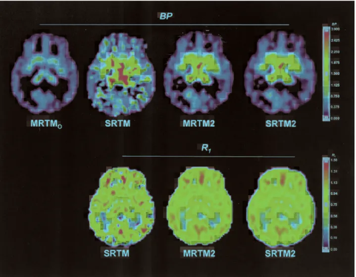
Fig. 9 shows examples ofBPand R1parametric im-ages estimated by MRTM2 and the corresponding mag-netic resonance images from the same subject. In theBP

images, voxels with correspondingR1values below 0.45 were set to 0. In this subject, all of these voxels belonged anatomically to the white matter region on the coregis-tered magnetic resonance scan (data not shown). This process improved the appearance of white matter regions in the BP image by removing the misleading noise-induced high BP values. The BP images (left column) show that regionallyBPvalues are high in the hypothala-mus and raphe, moderately high in the thalahypothala-mus and striatum, and low to very low in the amygdala and ce-rebral cortex, respectively. This regionalBPpattern was consistent with the known regional distributions of SERT sites. TheR1images (middle column) show that

R1values are high to moderate in the cortex, striatum and

thalamus; and relatively low in the hypothalamus, raphe and amygdala, respectively. This regional R1 pattern was consistent with human imaging studies of cerebral blood flow.

The thresholdR1value of 0.45 removed 1,800 ± 400 voxels (∼70 mL) from the white matter and the resulting

BPimages were visually considered satisfactory in six of eight subjects. There were a few white matter voxels with noise-induced moderately highBPin one of the two remaining subjects. In this subject, raising the threshold value to 0.47 removed those misleading voxels. In an-other subject, the thresholding process produced several sharp edges around the gray matter structures with rela-tively low flow such as the raphe and hypothalamus, although there were no misleading high-BPvoxels in the white matter. In this subject, lowering theR1 threshold value to 0.42 improved the white matter image appear-ance by removing the sharp edges without reintroducing any visually misleading high-BPvoxels.

FIG. 8. Parametric images of [11_{C]DASBBP(top row) estimated by MRTM}

O, SRTM, MRTM2, and SRTM2, andR1(bottom row)

estimated by SRTM, MRTM2, and SRTM2.BP, binding potential;R1, relative delivery; MRTMOand MRTM2, original multilinear reference

tissue model and its rearranged two-parameter model, respectively; SRTM and SRTM2, simplified reference tissue model and its two-parameter model, respectively.

DISCUSSION

In the present study, we applied two strategies to the original multilinear reference tissue model, MRTMO, to improve parametric images of BP and R1 for human [11C]DASB PET data. First, rearrangement of the MRTMO operational equation removed a noisy tissue radioactivity term,C(T), from the independent variables,

and this MRTM decreased the bias of BP estimation substantially, at the expense of considerably increased variability. The three-parameter linear method, MRTM, has similar parameter estimation characteristics to the three-parameter nonlinear method, SRTM (Lammertsma and Hume, 1996). Although this increasedBPvariability with MRTM over MRTMOdid not allow stableBP es-timations at the voxel level, MRTM did allow estimation

FIG. 9. Parametric images of [11_{C]DASBBP(left column) andR}

1(center column) estimated by MRTM2, and T1-weighted magnetic

resonance images (right column). In theBPimages, all voxels with correspondingR1values below 0.45 were set to zero. The top three

rows show transverse images and the bottom row shows sagittal images. TheBPimage in the second row corresponds to the MRTM2

BPimage in Fig. 8. The color display ranges forBP andR1images are 0 to 3.0 and 0 to 1.50, respectively. Am, amygdala; Hy,

hypothalamus; Ra, raphe complex; St, striatum; Th, thalamus;BP, binding potential; R1, relative delivery; MRTM2, two-parameter

ofk⬘2with little bias (<1%) and relatively small variabil-ity (<6%) from cerebellar and several tissue ROI data. Second, assuming that there is only onek⬘2value for the reference region, the number of parameters to estimate was reduced from three in MRTM to two in MRTM2 by using a common value ofk⬘2, in a manner analogous to that used in the nonlinear method SRTM2 (Wu and Car-son, 2002). MRTM2 substantially decreased the bias and variability ofBPandR1estimations over the linear and nonlinear three-parameter estimation methods. Further-more, the linearized approach allowed rapid generation (<15 seconds) of stable parametric images ofBPin the gray matter andR1in the whole brain.

We previously evaluated the effects of the first strat-egy used here for the estimation of the distribution vol-ume with plasma input function data for two neurorecep-tor radioligands, [18F]FCWAY and [11C]MDL 100,907 (Ichise et al, 2002). The resulting linear model (referred to as MA1 in that study) was also nearly identical to its nonlinear counterpart forVestimation at the voxel level. Like MRTM2, the operational equation for MA1 has only two parameters to estimate. However, for estima-tion of BP without blood data, an additional parameter appears in the operational equations for both linear and nonlinear reference tissue models, which causes param-eter estimation to be less stable under certain circum-stances. Therefore, the second strategy of determining a single value for the reference region clearance constant and reducing the number of parameter from three to two was applied for these reference tissue models.

SRTM2 has been developed by Wu and Carson (2002) and evaluated in comparison with SRTM for three ra-dioligands, [18F]FCWAY (5-HT1A), [

11

C]flumazenil (benzodiazepine), and [11C]raclopride (dopamine D2), where the magnitude of improvement in parameter esti-mation by eliminating one parameter depended on the radioligand’s kinetics. In that study, the largest impact of SRTM2 onBPestimation was found for [11 C]flumaze-nil, particularly with a 30-minute scan duration, where

BP variability was reduced from ∼10 to ∼5% and R1 variability was reduced by a comparable degree. SRTM2 had a similar pattern of impact for [11C]DASB in the present study, although the magnitude of BP noise re-duction was even larger.

To understand this behavior, consider the characteris-tics of the 1T model. Information in the data pertaining to

VorBPis obtained at later times, as each tissue region approaches transient equilibrium with the plasma. Math-ematically, this follows the function [1 − exp(−k2t)] as it approaches the value 1. In this framework, ignoring dif-ferences in the input function, a 90-minute [11C]DASB scan has kinetically similar characteristics to a 30-minute [11C]flumazenil scan, by having a similar value ofk2tat the end of the study. For [11C]DASB in the raphe,k2⳱ 0.013 min−1,t⳱90 minutes, andk2t⳱1.17, whereas

for [11C]flumazenil in the occipital cortex, k2⳱ 0.040 min−1,t⳱30 minutes, andk2t⳱1.20. This comparison also clarifies why, for [11C]DASB, the variability of voxel BP estimates in the raphe (20%) by SRTM2 or MRTM2 was larger than that in the striatum (12%), wherek2t⳱2.04 (Fig. 1A). This explanation is consis-tent with the corresponding larger C-R variability values for raphe of 18% compared with 12% for striatum (Table 3). Thus, a [11C]DASB scanning duration of more than 90 minutes may further improve parameter estimation at the voxel level for regions with very highBPsuch as the raphe, although Ginovart et al. (2001) showed that a 90-minute study is probably adequate for ROI-based [11C]DASB analyses.

We used the Cramer-Rao lower bound as a prediction of the minimum possible variance that can be achieved by unbiased estimators. Minimum-variance unbiased es-timators are generally desirable, and least-squares esti-mators usually have these characteristics for linear models (i.e., when the model equations are linear with respect to all the parameters). For nonlinear models, these characteristics are achieved asymptotically (i.e., for low noise). Thus, for nonlinear models, as noise in-creases, the estimators become biased and the variance diverges from the C-R bound. This can be seen in Table 3 by comparing the BP variability values for SRTM and SRTM with their respective C-R values with increas-ing noise. Note that divergence of the sample variance from the C-R variance occurs at different noise levels depending on the model and the parameter values. For example, at 15% noise for striatumBP(Table 3), sample variability for SRTM is dramatically higher than the C-R bound, whereas the SRTM2 sample variability agrees with its theoretical prediction. Also, the R1 parameter, which appears linearly in the model (Eq. 4), shows an excellent match between sample and C-R variability up to the highest noise levels for SRTM and SRTM2 (Table 4).

From a statistical point of view, the multilinear esti-mators MRTMO, MRTM, and MRTM2 are not mini-mum-variance unbiased estimators, because of the use of noisy dataC(T)in the independent variables (Eqs. 1–3). However, as shown in the Results, the magnitude of bias and variance depends considerably on the structure of the model and the parameter values. MRTMOproduces es-timates with large bias and variability smaller than the C-R bound. MRTM generally matches the bias and vari-ance of its nonlinear version, SRTM. However, an inter-esting estimation condition occurs for MRTM in the frontal cortex. Because of the small BP value, there is little difference between the frontal cortex and cerebel-lum TACs (Fig. 1), and the three-parameter estimation (Eqs. 2 and 4) is unstable. This instability produces dif-ferent results between the nonlinear SRTM and the linear

MRTM. This can be seen in the higher MRTMBP vari-ability compensated by lower MRTMR1variability. This effect is due to the high correlation between the first and second independent variables in Eq. 2 for the frontal cortex. Alternatively, MRTM2, while technically not a minimum-variance unbiased estimator, provides identi-cal estimation characteristics for all regions to the cor-responding NLS method SRTM2 for [11C]DASB (Ta-bles 3 and 4). It is likely that similar statistical results can be obtained with MRTM2 for other ligands that follow 1T kinetics.

In the simulations, we used a noise-free reference tis-sue TAC for the reference tistis-sue methods and a noise-free plasma input function for 1TKA. Noise in a refer-ence TAC or plasma input curve would have a global effect on the estimates (i.e., all voxel or ROI estimates for that subject would be affected in a common way). Therefore, this noise would not be reflected in the statistical noise of the image, as estimated in the sim-ulation (Tables 3 and 4, Figs. 2 and 4). Rather, this source of noise would increase intersubject variation and degrade the reproducibility of parameter measure-ments. In our PET data, the intersubject variability of 1TKA and MRTM2 results were comparable, suggesting that these noise sources are either small or of compar-able magnitude.

The simulation results for 1TKA were numerically identical to those of SRTM2 to three significant digits because (1) the operational equation SRTM2 (Eq. 4) is simply a different parameterization of Eq. 5 for 1TKA; (2) for the SRTM2 simulations, the true value ofk⬘2was used; and (3) for the 1TKA simulations, the true values ofK⬘1andk⬘2were used for calculation ofBPandR1. The subtle differences between the two methods were due to slight numerical integration errors of either the reference tissue TAC or plasma TACs. However, for the human PET data, 1TKA and SRTM2 were no longer identical because of the effects of input function measurement errors on 1TKA and differences ink⬘2determination be-tween the two methods.

There are a number of technical issues involved in implementing these methods. Both MRTM2 and SRTM2 require accuratea prioriestimation ofk⬘2. The simulation results indicated that k⬘2 estimation by MRTM using a single-tissue ROI such as the striatum has moderate vari-ability (10%) of k⬘2estimates, although the bias is very small (<1%). This noise in an individual’s k⬘2 estimate would translate into a bias in allBPandR1values for that subject (Fig. 6). To reduce this noise, we estimated k⬘2 values for several tissue ROIs and used a weighted mean of these values for MRTM2 and SRTM2. This strategy reduced the effective variability ofk⬘2estimates to less than 6%. Alternatively, Wu and Carson (2002) used the median value of estimated by SRTM for all brain voxels with moderate to highBP. The use of the median was

necessary in their case to avoid bias induced by the noise of each pixel TAC. The median was not required here, using an ROI-based approach for k⬘2 estimation. Use of the nonlinear SRTM for this purpose can be computa-tionally time consuming, and MRTM could be used in-stead to improve the processing speed. In any case, the optimal approach for MRTM or SRTM k⬘2 estimation should be carefully evaluated for each neuroreceptor ra-dioligand of interest.

For the white matter with very lowBP, voxel-wiseBP

estimation by MRTM2 was somewhat unstable, although MRTM2 reduced white matter noise considerably com-pared with SRTM (Figs. 5 and 8). To improve the ap-pearance of the white matter in the MRTM2BPimage, we used a simple threshold based on a fixed R1value. The disadvantage of this approach is that an appropriate thresholdR1value may differ between subjects (see Re-sults). By increasing the thresholdR1value, sharp edges appeared around gray matter structures with relatively low blood flow, such as the raphe and hypothalamus, because R1values in the neighboring voxels are below the threshold owing to the partial volume effect. An al-ternative approach to settingBPto 0 forR1values below a specific cutoff would be to add a constraint to the least-squares fitting, so that parameter estimates are lim-ited to a bounded region in parameter space (Fig. 5). This can be implemented with a two-step procedure, whereby voxels falling outside the permitted space can be refit to find the LS parameter values that fall on the boundary of the permitted space.

To minimize any bias introduced by the integral(s) on the right-hand side of the operational equations (Eqs. 1–4), the sampling rates used in the simulations were twice the rates used in the actual PET data. In addition, the first time point was excluded from fitting. This re-sulted in bias of no more than 0.1% for all methods in

BP,R1, andk⬘2estimations with noise-free data (Tables 2–4). Reduction of the sampling rates to those of actu-al PET data (27 frames) increased the magnitude of bias to approximately 0.3% for all models. Thus, for [11C]DASB, a very high sampling rate is not necessary to avoid integration-induced bias.

In this study, parameter estimation was performed without data weighting. However, MRTM2 (Eq. 3), SRTM2 (Eq. 4), and 1TKA (Eq. 5) can all be applied using weighted least squares estimation to account for noise-level differences inC(T) (Carson, 1986). Using the ideal weights, 1/Var[C(T)], for the current simulated data, weighted least squares improved the bias and vari-ability ofBPandR1estimations by MRTM2 and SRTM2 slightly across all noise levels. For example, theBPbias and variability in the raphe by SRTM2 at 15% noise were 2.5% and 16.0% with weighted least squares, and 3.6% and 20.5% unweighted, respectively. Thus, weighted least squares improves parameter estimation