How Has Environment Mattered?
An Analysis of World Bank Resource Allocation*
Anjali Acharya, Ede Jorge Ijjasz-Vasquez, Kirk Hamilton
Environment Department
Piet Buys, Susmita Dasgupta, Craig Meisner, Kiran Pandey, David Wheeler
Development Research Group
World Bank
World Bank Policy Research Working Paper 3269, April 2004
The Policy Research Working Paper Series disseminates the findings of work in progress to encourage the exchange of ideas about development issues. An objective of the series is to get the findings out quickly, even if the presentations are less than fully polished. The papers carry the names of the authors and should be cited accordingly. The findings, interpretations, and conclusions expressed in this paper are entirely those of the authors. They do not necessarily represent the view of the World Bank, its Executive Directors, or the countries they represent. Policy Research Working Papers are available online at http://econ.worldbank.org.
* For valuable comments and suggestions, our thanks to Kristalina Georgieva, Magda Lovei, Ken Chomitz, Franck Lecocq and the members of the World Bank's Environment Sector Board. The research summarized in this paper has been jointly supported by the World Bank's Environment Department and Development Research Group
Public Disclosure Authorized
Public Disclosure Authorized
Public Disclosure Authorized
Public Disclosure Authorized
Executive Summary
How has environment mattered for the World Bank? The aggregate figures suggest that it has mattered a great deal, since the Bank's total environmental lending has exceeded $US 9 billion over the past six years. In this paper, we use newly-available data to address a more precise version of the question: Across countries and themes, how well have the Bank's environmental lending and Analytical and Advisory Activities (AAA) matched the incidence of environmental problems? For our assessment, we extend our previous work on local pollution and fragile lands (Buys, et. al., 2003) to consideration of global emissions, biodiversity, water resources and institutional development. We
construct cross-country problem indicators for each environmental theme, and combine them with country risk measures to estimate optimal thematic lending and AAA for each country. Then we compare our estimates with actual lending and AAA to assess the match between environmental problems and the Bank's response.
We begin by constructing an overall indicator of environmental problems from our thematic indicators. Using regression analysis, we find a strong relationship between countries’ general indicator values and the scale of their environmental borrowing, but a relatively weak relationship for AAA. At the thematic level, we find that problem indicators have relatively weak relationships with both lending and AAA. Adding country risk to the analysis, we test an optimal allocation model and find that it is consistent with the Bank’s actual lending and AAA since 1998. We conclude that our model’s assignment of lending and AAA to countries reflects the Bank’s actual experience with partner countries. The model’s explanatory power is relatively low, however, and when we compare model assignments to actual allocations, we find many large discrepancies for countries and environmental themes. Some gaps may reflect activity by other donor institutions, but many others may represent problems with efficient implementation of the Bank’s Environment Strategy. To promote further discussion of this issue, we use our optimal allocation model to develop measures of lending opportunity by environmental theme for the Bank's partner countries.
1. Introduction
The World Bank has become the world's largest source of financing for
environmental improvement in developing countries. During the period 1998 - 2003, the Bank lent approximately $US 9.2 billion for environmental purposes in 381 projects.1 The scale of this activity indicates that environment has mattered a great deal to the Bank and its partner countries. Until recently, however, data scarcity has prevented a more detailed assessment of the Bank's environmental operations. In this paper, we use newly-available information to ask how, more precisely, environment has mattered: Across countries and themes, how well has the Bank's allocation of resources for lending and Analytical and Advisory Activities (AAA) matched the incidence of environmental problems? The analysis extends our previous work on local pollution and fragile lands (Buys, et al., 2003) to consideration of global emissions, biodiversity, water resources and institutional development. We construct a cross-country problem indicator for each environmental theme, and assess the match between thematic resource allocation and problem incidence. To assist in promoting a closer match, we also combine our
environmental indicators with information on country risk to estimate optimal resource allocation across countries.
The remainder of the paper is organized as follows. Section 2 introduces our environmental indicators, and Section 3 provides a measure of country risk. Section 4 describes the Bank's environmental accounting information. In Section 5, we assess the match between country lending and the general scale of countries' environmental problems. Section 6 extends the analysis to thematic lending. Section 7 introduces our
1 This estimate by the Bank's Environment Department includes environmental components of loans in other sectors (e.g., transport, agriculture), as well as loans that are attributed to the environment sector.
optimal allocation model, with a brief review of the methodology developed in Buys, et al. (2003). Assuming continuity with the past scale and thematic composition of lending, Section 8 uses the model to estimate lending and AAA opportunities by country and environmental theme for the period 2004-2009.2 Section 9 interprets our findings using two country cases, and Section 10 provides a summary and conclusions.
2. Environmental Indicators
Building on prior work by Buys, et al. (2003), we construct country indicators for six environmental problems: greenhouse gas emissions; health damage from air and water pollution; the threat of natural resource degradation on fragile lands; threats to biodiversity; problems related to water resources; and problems with environmental policies and institutions. All of our indices reflect recent research on the cross-country incidence of environmental problems.
For global greenhouse gas emissions, our indicator is total metric tons of carbon-equivalent in 2000 from fuel combustion (CO2), land-use change (CO2) and other sources (methane (CH4), nitrous oxide (N20), hydrofluorocarbons (HFC’s), perfluorocarbons (PFCs), and sulfur hexafluoride (SF6)). We draw our emissions estimates from the World Resources Institute’s Climate Analysis and Indicators
database.3 Our estimate of pollution damage is total DALY (disability-adjusted life year) losses from air and water pollution. We draw our DALY estimates from recent research
2 The supporting database and an accompanying atlas can be downloaded from the Environment Department (lnweb18.worldbank.org/ESSD/envext.nsf/41ByDocName/Environment), or from the Development Research Group (www.worldbank.org/nipr).
3 The World Resources Institute’s Climate Analysis and Indicators database is available online at http://cait.wri.org.
by the World Bank, in collaboration with WHO (Pandey, et al., 2004; Wang, et al., 2003).
For natural resource degradation, we base our indicator on recent research that identifies the vulnerability of people on fragile lands (i.e., land that is steeply-sloped, arid, or covered by natural forest) as a major determinant of rural poverty and natural resource degradation in developing countries (World Bank, 2003). Our indicator, the total rural population living on fragile lands, has been constructed from a GIS
(Geographic Information System) - based spatial overlay of demographic, topographical, climatic and natural resource information.
We have developed our biodiversity threat indicator from a variety of sources. For terrestrial biodiversity, we use a GIS-based spatial overlay of human population with critical areas identified by Conservation International (CI), the World Wildlife Fund (WWF), and Birdlife International (BI). We also include freshwater lake areas, to capture the role of inland aquatic ecosystems. The World Bank’s Environment Strategy focuses on both the threat to biodiversity from human encroachment, and the value of biodiversity resources for human populations. Our indicator for this two-way
relationship in each country is its total human population in critical biodiversity areas. For marine biodiversity, we draw on estimates of reef ecosystems at risk by Bryant, et al. (1998). Summing across all endangered reefs, we use each country's share of the total as our index of marine biodiversity threat. While terrestrial and marine threats are quite distinct geographically, we create a composite indicator to match the Bank's thematic
category (biodiversity conservation). Since the two indices are weakly correlated (ρ = .27), assignment of relative weights has a significant impact on the result. We assign equal weights, because we have no scientific basis for a differentiated weighting scheme.
To construct a water-resource indicator, we draw on two sources of information. The first is an estimated geographic distribution of excess demand for water resources (surface and sub-surface) in Vörösmarty, et al. (2000). We use GIS to compute the total population residing in excess-demand areas identified by this research. The second information source is a database of deaths and injuries from floods maintained by the Centre for Research on the Epidemiology of Disasters (CRED, Université Catholique de Louvain). For each of the Bank's partner countries, we calculate the sum of deaths and injuries for all recorded floods since 1960. In constructing an indicator for flood damage, we weight deaths to injuries in the ratio 50:1. Using equal weights, we combine our indicators for demand pressure and floods into a composite indicator of water-related problems.4
We derive our indicator for environmental policy and institutional problems from two sources. The first is the World Bank's Country Policy and Institutional Assessment (CPIA) database, which rates environmental policies and institutions on a numerical scale of 1 (the lowest) to 6. For this exercise, we reverse the scaling (1 becomes the highest) and normalize the ratings so that countries with the greatest problems score 100. To proxy the scale of the problems confronted by environmental institutions, we compute the mean value of our five thematic indicators (global emissions, pollution, natural resource degradation, biodiversity threats, water-related problems).5,6 To assure equal weighting
4 Our index of demand pressure also provides a useful proxy for economic damage from drought conditions. We are indebted to our colleagues in the Bank’s Middle East / North Africa region for this observation.
5 While the CPIA ratings provide useful information for comparing institutional needs, they are not sufficient for judging investment priorities because they do not account for differences in the scale of environmental problems faced by a country's institutions. If Brazil and Bhutan receive the same CPIA rating, for example, ignoring their scale difference will lead to assignment of identical lending in the optimization model.
6 We recognize that an equal-weighted index is only one of numerous plausible indicators for general environmental problems. In Appendix 2, we develop alternative indices and analyze their association with
with the institutional rating, we normalize this mean indicator to the range [0 - 100]. Our composite indicator is the product of the normalized environmental index and CPIA rating.
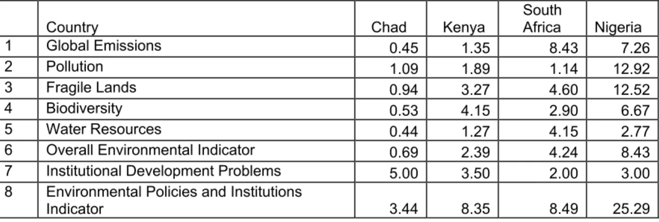
Table 2.1 illustrates the calculation of the policies and institutions indicator for four countries in Sub-Saharan Africa. This indicator (row 8) equals the product of the
indicator of institutional development problems (row 7) and the indicator of overall environmental problems (row 6). The latter is the average of problem indicator values for global emissions, pollution, fragile lands, biodiversity and water resources. The four country cases illustrate the contributions of separate components to the final indicator values. Chad has a low overall environmental indicator (.69) but a very high institutional indicator (5), yielding a product of 3.44. South Africa’s overall environmental indicator (4.24) is about six times Chad’s value, but its institutional indicator (2) is much lower because its institutions are more highly-developed. The resulting composite indicator for South Africa (8.49) is about 2.5 times Chad’s indicator value (3.44). Kenya has about the same composite indicator value as South Africa (8.35), but the indicator components are quite different. Kenya’s environmental indicator (2.39) is somewhat more than half of South Africa’s (4.24), but Kenya’s institutional problem indicator (3.5) is about 1.8 times South Africa’s. As a result, the products of the two indicators are nearly the same for the two countries. Of the four countries, Nigeria has by far the largest composite indicator value (25.29) because of the size of its overall environmental indicator (8.43).
the equal-weighted index. Our results show that correlations among the indicators remain at .95 or higher, over a broad range of plausible definitions.
Table 2.1 Environmental Policies and Institutions Indicators for Four African Countries Country Chad Kenya South Africa Nigeria 1 Global Emissions 0.45 1.35 8.43 7.26 2 Pollution 1.09 1.89 1.14 12.92 3 Fragile Lands 0.94 3.27 4.60 12.52 4 Biodiversity 0.53 4.15 2.90 6.67 5 Water Resources 0.44 1.27 4.15 2.77 6 Overall Environmental Indicator 0.69 2.39 4.24 8.43 7 Institutional Development Problems 5.00 3.50 2.00 3.00 8 Environmental Policies and Institutions
Indicator 3.44 8.35 8.49 25.29
3. Country Experience with Project Implementation
The World Bank lends to countries that have highly-varied experiences with implementation. To incorporate this factor, we draw on a database maintained by the World Bank's Operations Evaluation Department (OED). The database rates the
outcomes of 3,075 World Bank projects implemented in 146 countries since 1990. OED rates projects in eight categories: highly satisfactory, satisfactory, moderately
satisfactory, marginally satisfactory, marginally unsatisfactory, moderately
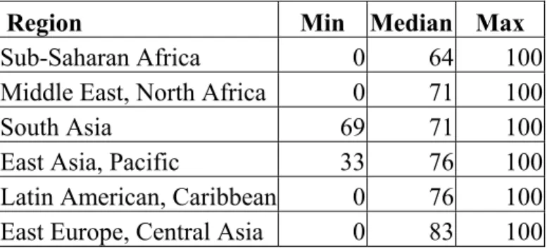
unsatisfactory, unsatisfactory, and highly unsatisfactory. We interpret the highest two ratings as "successful" for our purposes, and define our country risk indicator as the percentage of projects rated successful by OED. Table 3.1 displays the distribution of our results by region. Although the estimated success rates are generally highest in Eastern Europe/Central Asia and lowest in Sub-Saharan Africa, countries in all Bank regions except South Asia exhibit a wide range of variation.
Table 3.1: Distribution of Country Probabilities of Project Success, by Region
Region Min Median Max
Sub-Saharan Africa 0 64 100 Middle East, North Africa 0 71 100 South Asia 69 71 100 East Asia, Pacific 33 76 100 Latin American, Caribbean 0 76 100 East Europe, Central Asia 0 83 100
4. Environmental Resource Allocation by the World Bank
The World Bank's Environment Department has recently completed an accounting of environmental lending and AAA in seven thematic categories: climate change, pollution management, land management, biodiversity, water resource management, environmental policies and institutions, and other environmental management. This exercise has drawn on recent changes in the Bank's accounting system, which now tracks the allocation of funds across both sectors (e.g., environment, infrastructure) and themes within sectors (e.g., climate change, pollution management). The new system identifies the environmental components of projects whose sectoral identification is
non-environmental. For example, transport-related projects often include components that promote reduction of vehicular air pollution.
This paper draws on information for all World Bank projects approved since FY 1998, and all AAA since FY 2000. Using the appropriate thematic codes, we calculate total Bank lending and AAA by country and environmental theme. Our five
environmental indicators and the institutional problem indicator are constructed to match the corresponding thematic categories in the project database. The seventh thematic
category (other environmental management) has no direct analog, so we use the mean value of the five environmental indicators for our matching exercise.
Perhaps the most striking feature of the Bank's environmental lending is the
stability of its thematic allocation over time.7 As Figure 4.1 shows, annual environmental lending declined from around $3.5 billion in FY 1993 to $1.0 billion in FY 2003.
Despite this sharp change in aggregate lending, the regression results in Table 4.1 suggest that thematic shares remained stable: None exhibits a significant time trend since 1993. Figure 4.1 World Bank Environmental Lending, 1993-2003 ($US Million)
0 500 1,000 1,500 2,000 2,500 3,000 3,500 4,000 1993 1995 1997 1999 2001 2003 Fiscal Year
Total Environmental Lending
______________________________________________________________________________ Table 4.1: Trend Tests for Thematic Shares
Climate Pollution Land Biodiversity8 Water Policy Other
Time 0.318 -0.167 0.639 0.074 0.008 -1.071 0.199 (0.63) (0.19) (1.38) (0.37) (0.01) (1.65) (1.09) Constant 8.337 33.404 8.529 2.215 20.456 24.930 2.128 (2.44)* (5.54)** (2.72)* (1.61) (5.86)** (5.67)** (1.71) Obs. 11 11 11 11 11 11 11 R-squared 0.04 0.00 0.17 0.01 0.00 0.23 0.12
Absolute values of t statistics in parentheses * significant at 5%; ** significant at 1%
______________________________________________________________________________
Produced by thousands of interactions between the Bank and its partner countries, these results suggest very strong continuity in the relative valuation of thematic
objectives. We will return to this point in Section 7, which develops a model for the optimal allocation of environmental resource allocation by the Bank.
5. How Has Environment Mattered in the Aggregate?
We begin our assessment by analyzing the match between environmental lending, AAA and environmental problems at the country level. Our overall environmental indicator is the mean of the five thematic indicators.9 We use log values for the analysis because the size distributions of country indicators and resource allocations are extremely
8 For biodiversity, our data include only Bank lending. Grants by the Global Environment Facility (GEF) for biodiversity conservation are not included in this analysis, but the GEF is currently conducting a parallel analysis of its own resource allocation.
9 All indicators are normalized to the range [0-100], so they have equal weight in determining the mean indicator.
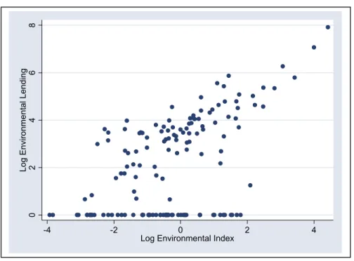
skewed.10 As the scatter plot in Figure 5.1 suggests, the association between overall environmental problems and lending is very strong for those countries that have received environmental loans.
Figure 5.1: World Bank Environmental Lending vs.
Overall Environmental Problems (Log Scale)
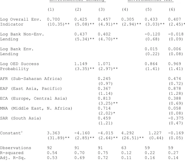
In a log-log regression of environmental lending on the overall environmental indicator (Table 5.1, column 1), the estimated response elasticity is .70, with an
associated t-statistic of 10.3 and regression R2 (adjusted for degrees of freedom) of .53.
10 Conventional regression and correlation analysis assume that variable distributions do not contain extreme “outlier” observations, because such outliers can sharply skew the results. In this case, both nominal and per-capita distributions are extremely skewed. Log measures, on the other hand, have regular, approximately-normal distributions with no outliers.
0 2 4 6 8 Log E n vironment al Lending -4 -2 0 2 4
Table 5.1: Determinants of Environmental Lending
Environmental Lendinga Environmental AAAb
(1) (2) (3) (4) (5) (6)
Log Overall Env. 0.700 0.425 0.457 0.305 0.433 0.407
Indicator (10.35)** (5.08)** (4.91)** (2.94)** (3.03)** (2.45)*
Log Bank Non-Env. 0.437 0.402 -0.120 -0.018
Lending (5.34)** (4.70)** (0.68) (0.09)
Log Bank Env. 0.015 0.006
Lending (0.22) (0.08)
Log OED Success 1.149 1.071 0.864 0.969
Probability (3.35)** (2.97)** (1.41) (1.41)
AFR (Sub-Saharan Africa) 0.245 0.474
(0.97) (0.72)
EAP (East Asia, Pacific) 0.367 0.878
(1.14) (1.28)
ECA (Europe, Central Asia) 0.813 0.388
(3.25)** (0.69)
MNA (Middle East, N. Africa) 0.714 0.058
(2.02)* (0.08)
SAR (South Asia) 0.459 -0.375
(1.21) (0.47) Constantc 3.363 -4.160 -4.015 4.292 1.227 -0.169 (31.89)** (2.85)** (2.64)** (26.51)** (0.44) (0.05) Observations 92 91 91 63 59 59 R-squared 0.54 0.70 0.75 0.12 0.22 0.27 Adj. R-Sq. 0.53 0.69 0.72 0.11 0.16 0.14
Absolute value of t statistics in parentheses significant at 5%; ** significant at 1%
a Limited to countries with environmental lending n Limited to countries with environmental AAA
c LCR (Latin America, Caribbean) is the excluded regional dummy variable.
___________________________________________________________________________ This result suggests that a 1% increase in overall environmental problems is associated with a .70% increase in environmental lending. At the regional level, Figure 5.2 also suggests a good correspondence between overall environmental problems and environmental lending in countries where such lending has occurred. The relationship is very strong in East and South Asia (EAP, SAR), but it is also apparent in the other
regions. However, all regions (particularly AFR and LCR) include countries that have no lending, despite significant environmental problems.
Figure 5.2: World Bank Environmental Lending by Region vs. Overall Environmental Problems (Log Scale)
The number of such zero-lending cases suggests that the Bank's interaction with these countries has been affected by other factors. We introduce broader considerations into our regressions by including the Bank's total country lending and countries' OED project success rates, as well as regional differences. The results in columns 2 and 3 of Table 5.1 suggest that the Bank's overall lending relationship with a country and the country's project success rate are both significant determinants of environmental lending. The results in column 3 also indicate a significant component of environmental lending to two regions (ECA, MNA) that is not accounted for by our environmental problem
indicator, project success rates, or other Bank lending.
0 2 4 6 8 0 2 4 6 8 -4 -2 0 2 4 -4 -2 0 2 4 -4 -2 0 2 4
AFR EAP ECA
LCR MNA SAR
Log Env
ironmental Lending
Log Environmental Index
Our results for total Bank lending are uniformly significant at the 99% level, and the results for the OED ratings are significant at the 95% level or higher. The parameter estimates suggest that a 1% increase in Bank lending is associated with a .4% increase in environmental lending, and a 1% increase in the OED rating is associated with an
environmental lending increase of about 1%. Once we control for these two factors, environmental problems retain a significant impact on environmental lending at the 99% level. However, the estimated response elasticity drops from .70 to around .45.
The results for AAA in Figure 5.1 are quite different from the results for lending. The association with environmental problems is uniformly significant at the 99% confidence level, but we find no significance for environmental lending, non-environmental lending, the OED success probability, or any regional dummies.
R-squares for the AAA regressions are much lower than R-R-squares for lending, suggesting a much greater random component in the allocation of AAA resources.
6. Allocation by Environmental Theme
From an institutional perspective, our overall results for lending are encouraging because they suggest that large, politically-difficult reallocations across countries would not generally be necessary to bring country lending into alignment with overall
environmental problems. The implications for AAA may be more serious, since our results suggest that the association between AAA and environmental problems explains only a small component of the cross-country variation in AAA.
We extend the analysis to the thematic level, by regressing lending and AAA for each theme on the associated environmental problem indicator (Table 6.1). The results for lending suggest strong relationships that mirror the overall relationship captured by
Table 5.1 For each of the six themes, lending is positively associated with the relevant indicator at a very high level of significance. Estimated elasticities are generally near 0.5, except for biodiversity (0.3) and policies and institutions (1.2). However, the low R-squares suggest that most thematic lending is determined by other factors. For AAA, the results are even weaker. Regression R-squares are extremely low, and thematic AAA is not significantly associated with the relevant thematic indicator in 3 of 6 cases. We find positive, significant associations for climate change, water resources and policies and institutions.
Overall, the relationship between AAA allocations and indicator values appears to be nearly random. Although our results indicate significant relationships between lending and environmental problems, the low R-squares also imply considerable scope for better matching between needs and resources. In the following sections, we develop and implement a model that we believe can assist in this task.
7. Optimal Thematic Lending and AAA
Following Buys, et. al (2003), we model the welfare impact of World Bank investments as a function of their levels and distributions across countries. We recognize that the Bank must strike a balance between country representation and global welfare maximization in its resource allocation decisions. To reflect this balance, we assume that the Bank's welfare function is characterized by unit-elastic substitution across countries. A unit-elastic (Cobb-Douglas) function permits tailoring of programs to a country's circumstances, while
encouraging portfolio diversification through the operation of diminishing returns. In our model, expected welfare gains from Bank investments are related to both thescale of a
Table 6.1: Regression Results: Thematic Lending, AAA and Environmental Indicators Environmental Thematic Lending vs. Thematic Indicator Values
(Limited to Countries with Environmental Lending)
Climate Pollution Land Biodiversity Water Policies Log Environmental Indicators Climate 0.469 (2.86)** Pollution 0.460 (3.30)** Land 0.459 (3.18)** Biodiversity 0.320 (3.32)** Water 0.553 (4.33)** Policies 1.214 (6.26)** Constant -2.519 0.686 -0.572 -2.907 0.115 -0.996 (7.51)** (1.80) (1.53) (10.56)** (0.30) (3.09)** Observations 92 92 92 92 92 91 R-squared 0.08 0.11 0.10 0.11 0.17 0.31 Adj. R-Sq. 0.07 0.10 0.09 0.10 0.16 0.30
Environmental Thematic AAA vs. Thematic Index Values (Limited to Countries with Environmental AAA)
Climate Pollution Land Biodiversity Water Policies Log Environmental Indicators Climate 0.680 (3.18)** Pollution 0.297 (1.14) Land 0.367 (1.36) Biodiversity 0.144 (0.77) Water 0.522 (2.23)* Policies 1.131 (3.34)** Constant -3.142 -1.454 -2.653 -2.163 -0.379 -1.016 (8.05)** (2.87)** (5.98)** (4.68)** (0.74) (1.80) Observations 63 63 63 63 63 63 R-squared 0.14 0.02 0.03 0.01 0.08 0.15 Adj. R-Sq. 0.12 0.00 0.01 0.00 0.06 0.14
Absolute value of t statistics in parentheses * significant at 5%; ** significant at 1%
country's environmental problems and the probability that projects will be successful under local conditions. We assume that the Bank assigns the same opportunity values to human life, health and natural resource savings in all of its partner countries. From these assumptions, we derive a simple optimal allocation rule (Buys, 2003): For a particular environmental theme (e.g., pollution, threats to biodiversity), each country's optimal share of available lending and AAA resources is proportional to the product of its problem scale and the probability of project success.
Do our assumptions, and the resulting allocation rule, actually reflect the Bank’s operational experience? To check for general consistency, we have estimated cross-country equations in which the log of the Bank’s environmental lending and AAA are regressed on the logs of the overall environmental index and the OED measure of success probability (Table 7.1). Our simple allocation rule implies that the parameters of both variables are equal to one. Using the standard F-test for the lending and AAA equations, we find that these parameter values cannot be rejected at the standard significance level (5%) in either case. We conclude that the Bank’s environmental lending and AAA have been broadly consistent with our allocation rule. However, the high degree of
unexplained variation in both regressions suggests large gaps between actual and optimal allocation in many cases.
Our model addresses the allocation problem within each environmental theme, but it cannot determine thematic allocations from total lending resources. However, our historical results for thematic lending shares (Section 4) have strong significance in this context. The stability of these shares, in the face of sharp changes in total environmental lending, suggests a clear pattern of preferences underlying the Bank's many transactions
with partner countries. We accept these overall preferences, and assume that future
thematic lending shares will be identical to the lending shares for the period 1998 - 2003. Table 7.1: Tests of the Cobb-Douglas Allocation Rule:
Environmental Lending and AAA (Standard errors in parentheses)
Log Log
Lending AAA
Log Environmental Problem 1.136 1.265
Indicator (EPI) (0.18)** (0.21)**
Log OED Success Probability (OSP) 2.602 1.143
(0.73)** (0.87) Constant -9.960 -5.099 (3.09)** (3.67) Observations 139 139 R-squared 0.28 0.21 Adj. R-Squared 0.27 0.20 F [EPI = OSP = 1] 2.65 0.78 Prob. > F 0.07 0.46 significant at 5%; ** significant at 1% _____________________________________________________________
We also use the lending shares as guidelines for AAA, since the Bank’s analytical and advisory activities are supposed to serve its lending program.
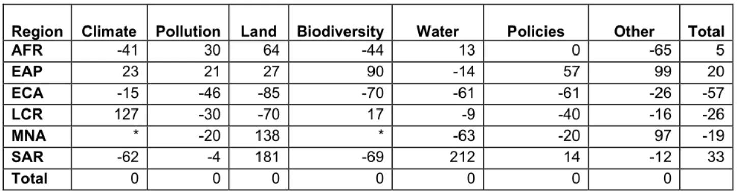
Table 7.2 presents percent changes associated with movement from actual to optimal lending by sector and region. In Sub-Saharan Africa, for example, the overall gap between actual and optimal environmental lending is small (+5%), but thematic gaps vary from around -40% for climate change and biodiversity to +64% for land. South Asia has a relatively large overall gap (+33%), and thematic gaps ranging from -60% or less for biodiversity and climate change to over +180% for land and water resources. In a strongly-contrasting pattern, Latin America and the Caribbean have a relatively large overall gap (-26%), with increases for climate change (+127%) and biodiversity (+17%) and decreases for land and water resources (-70% and -9%, respectively). Across
regions, moving from actual to optimal lending results in increases for Africa (5%), East Asia / Pacific (20%) and South Asia (33%), and decreases for Europe / Central Aisa (-57%), Latin America / Caribbean (-26%) and Middle East / North Africa (-19%). Table 7.2: % Differences Between Actual and Optimal Lendinga
Region Climate Pollution Land Biodiversity Water Policies Other Total
AFR -41 30 64 -44 13 0 -65 5 EAP 23 21 27 90 -14 57 99 20 ECA -15 -46 -85 -70 -61 -61 -26 -57 LCR 127 -30 -70 17 -9 -40 -16 -26 MNA * -20 138 * -63 -20 97 -19 SAR -62 -4 181 -69 212 14 -12 33 Total 0 0 0 0 0 0 0
a Estimates reflect changes from actual to optimal lending * Division by 0 in growth rate calculation
Tables 7.4 and 7.5 present % differences for AAA under two assumptions. Table 7.4 holds thematic AAA shares constant at their levels for 2000-2003, while Table 7.5
assumes that thematic AAA shares are equal to thematic lending shares for 1998-2003. The differences between the two tables are evident, reflecting the substantial differences between thematic shares for lending and AAA in Table 7.3. Lending shares are higher for climate, pollution, land and water, while AAA shares are higher for biodiversity and environmental policies and institutions. The difference for pollution is particularly striking (31% of lending vs. 10% of AAA).
Table 7.3: Thematic Shares for Lending (1998-2003) and AAA (2000-2003)
Resource Climate Pollution Land Biodiversity Water Policies Other
Lending 10 31 15 3 23 15 4
AAA 4 10 7 10 19 27 21
At the regional level, Tables 7.4 and 7.5 show that the change in assumptions makes little difference for allocations. Whether or not thematic lending shares are used for
AAA allocation, the pattern of regional change in AAA is similar to the pattern for lending (with the exception of Africa): Two regions have increases in AAA (East Asia / Pacific, South Asia) and four regions have decreases (Africa, Europe / Central Asia, Latin America / Caribbean and Middle East / North Africa). Furthermore, the magnitudes of overall regional changes are almost identical in Tables 7.4 and 7.5 (again, Africa excepted)
However, changing thematic shares from the AAA allocation to the lending
allocation has a large impact on thematic results. Moving to the lending allocation (Table 7.5) entails very large increases for three sectors (climate (118%), pollution (198%), land (107%) and large decreases for two (biodiversity (-73%), policies and institutions
(-44%)). Overall, combining these changes with regional shifts generates much larger regional % changes within sectors in Table 7.5 than in Table 7.4. In some cases, change patterns are replicated in the two tables (e.g., large % increases in climate, pollution and land for EAP; decreases for all themes except water in ECA). However, other patterns are reversed, particularly for biodiversity, which gets a much larger allocation in Table 7.4 (10% of total AAA) than in Table 7.5 (3% of total lending).
Table 7.4: % Differences Between Actual and Optimal AAA (AAA Thematic Shares Held Constant)
Region Climate Pollution Land Biodiversity Water Policies Other Total
AFR -35 20 -62 -75 -81 146 -56 -52 EAP 171 271 411 222 50 -8 88 61 ECA -63 -83 -65 -87 2 -66 -71 -68 LCR 473 64 -86 90 13 25 -26 -7 MNA -5 -59 279 -12 -69 19 -49 -39 SAR -62 9 2,273 100 366 59 1,313 144 Total 0 0 0 0 0 0 0 0
Table 7.5: % Differences Between Actual and Optimal AAA (AAA Thematic Shares = Lending Thematic Shares)
Region Climate Pollution Land Biodiversity Water Policies Other Total
AFR 42 258 -20 -93 -77 37 -92 -52 EAP 490 1,007 955 -14 76 -49 -67 56 ECA -20 -48 -28 -97 20 -81 -95 -66 LCR 1,150 388 -70 -49 33 -30 -87 -18 MNA 108 24 684 -76 -63 -34 -91 -37 SAR -17 224 4,804 -47 448 -11 146 166 Total 118 198 107 -73 18 -44 -83 0
Our results also suggest possible differences in the relative magnitudes of thematic changes for lending and AAA. Appendix Table 2 presents results for actual and optimal lending and AAA across sectors and regions. We estimate the relative magnitudes of thematic gaps by calculating the absolute values of regional thematic gaps as percentages of actual thematic allocations. For each theme, the sum of absolute-value percentage gaps provides an indicator of relative “misallocation”. Table 7.6 summarizes the results for three cases: lending, AAA (A -- with thematic AAA shares), and AAA (L -- with thematic lending shares). Both nominal and rank correlations suggest that misallocations are most closely matched for lending and AAA(A) shares; poorly matched for lending and AAA(L); and weakly matched for AAA(A) and AAA(L). We conclude that
statements about thematic misallocation are highly sensitive to the comparison standard, and general conclusions do not seem appropriate.
Table 7.6: Thematic Misallocation Measures Numerical data
Theme Lending AAA (A) AAA (L) Lending AAA(A) Climate 45 89 142 AAA(A) 0.67 Pollution 22 82 239 AAA(L) -0.32 0.45 Land 70 127 181 Biodiversity 68 105 73 Water 49 83 96 Policies 38 35 48 Ranks
Theme Lending AAA (A) AAA (L) Lending AAA(A) Climate 4 3 3 AAA(A) 0.89 Pollution 6 5 1 AAA(L) -0.09 0.26 Land 1 1 2 Biodiversity 2 2 5 Water 3 4 4 Policies 5 6 6
8. Future Opportunities for Thematic Lending
To assess future opportunities, we assume that total environmental lending during the period 2004-2009 will be identical to lending during 1998-2003 ($9.2 billion). For each country, the optimal share of environmental lending by theme is proportional to the product of the country's thematic indicator and its OED success probability. To calculate optimal lending, we multiply each country's optimal thematic share by total thematic lending for the period 1998-2003. Then we add across themes to obtain total optimal lending for each country. Recognizing that the Bank may limit its lending to some countries for a variety of reasons, we derive a control factor from lending experience during the past six years. Across countries, the maximum ratio of environmental loans to total loans was 46%. As Figure 8.1 shows, most ratios were 10% or less.
Figure 8.1: Size Distribution of Ratios: Environment Lending / Total Lending, 1998 - 2003
Setting the maximum ratio at 40%, we identify a country's future environmental lending opportunity as the lower of two numbers: our estimate of total optimal
environmental lending, or 40% of total lending during 1998 - 2003. With this control, the environmental lending opportunity is our optimal lending estimate for 83% of the 150 countries in our dataset. For the others, we use the 40% ratio to keep environmental lending within a plausible bound. Having determined the overall lending opportunity, we multiply by our optimal thematic shares to estimate thematic lending opportunities. We present the results in Appendix 1, with countries in each region sorted by total lending opportunity. The regional tables display historical lending, as well as future opportunities.
To illustrate, the six Sub-Saharan African countries with the highest
environmental lending opportunities are Nigeria ($144 million), Ethiopia ($128 million),
0 10 20 30 40 50
Ratio of Environmental to Total Lending (%)
0 20 40 60 80 100
Tanzania ($76 m.), Uganda ($38 m.), Mozambique ($35 m.), Congo DR ($32 m.), and Madagascar ($30 m.). Our results suggest that lending opportunities are generally largest for pollution management, although sizable opportunities also exist for land management, water resource management, and environmental policies and institutions. The mix of opportunities differs substantially by country, reflecting differences in their
environmental problems. Other regions exhibit similarly-diverse patterns. We summarize our results Table 8.1, which includes all countries with
environmental lending opportunities of $50 million or more during the period 2004-2009. Of the 23 countries listed, 7 are in the East-Asia Pacific Region (EAP), 4 in Latin
America and the Caribbean (LCR), and 3 are in each of the other regions. If, as we assume, AAA priorities should reflect lending priorities, then these same 23 countries should also form the core group for AAA during the period 2004-2009. AAA priorities for other countries would reflect the same rank-order as the lending opportunities in Appendix 1.
9. Interpretation of Results: Ethiopia vs. Nigeria
We provide an illustrative interpretation of our results by comparing the cases of Ethiopia and Nigeria in Table 9.1. Both have been among the Bank’s top borrowers in Sub-Saharan Africa: From 1998-2003, Nigeria borrowed $912 million and Ethiopia borrowed $1,381 million. Among the 48 Sub-Saharan countries, Nigeria’s overall environmental problem indicator ranks first and Ethiopia’s second. Both countries are in the midrange for the OED project success rate (45% for Nigeria; 65% for Ethiopia). After adjusting for success rates, Nigeria’s optimal lending is $144 million and Ethiopia’s is $128 million.
Table 8.1: Country Lending Opportunities, 2004-09 Region Country Lending Opportunity, 2004-09 ($ Million) EAP China 2,904 SAR India 1,405 EAP Indonesia 548 SAR Bangladesh 345 SAR Pakistan 299 LCR Brazil 241 LCR Mexico 186 ECA Russian Federation 153 AFR Nigeria 144 MNA Iran (Islamic Republic of) 140 EAP Philippines 138 EAP Vietnam 138 MNA Egypt, Arab Republic of 138 AFR Ethiopia 128 EAP Korea, Republic of 103 ECA Turkey 102 ECA Ukraine 99 EAP Thailand 93 LCR Argentina 87 EAP Malaysia 78 AFR Tanzania 76 LCR Peru 56
MNA Yemen, Republic of 50
With this information as background, it is instructive to compare actual total and thematic lending. Ethiopia’s actual lending is in the same range as its optimal lending: $159 million. As Table 9.1 shows, Ethiopia ranks high in all environmental indicator categories except climate change. However, the pattern of thematic lending bears almost no relationship to Ethiopia’s thematic rankings in Africa, or to its optimal thematic lending. Climate is the most obviously-divergent category, with optimal lending of $2.1 million and actual lending of $71.8 million. Lending amounts for pollution management
and land and water resource management are far lower than the optimal levels, while lending for policies and institutions is substantially higher.
Nigeria’s case is even more divergent than Ethiopia’s. Despite the highest ranking in Sub-Saharan Africa for environmental problems and $144 million in optimal lending, Nigeria’s actual lending is only $2.5 million. Two themes – pollution and water resource management – have very small loans, and the others none at all.
Table 9.1 Environmental Indicator and Lending Status of Ethiopia and Nigeria Within Sub-Saharan Africa
Climate Pollution Land Biodiversity Water Policies Overall Ethiopia Indicator Rank 11 2 3 2 3 2 2 Actual Lending 71.8 31.8 0.0 0.7 5.1 33.4 159.2 Optimal Lending 2.1 57.7 23.2 2.8 18.9 18.9 127.5 Nigeria Indicator Rank 3 1 1 3 4 1 1 Actual Lending 0.0 1.3 0.0 0.0 1.3 0.0 2.5 Optimal Lending 7.4 70.3 29.2 1.9 9.7 20.9 143.6
9. Summary and Conclusions
In this paper, we have used new environmental and accounting information to address four questions about the World Bank's environmental lending:
(1). Have the Bank's patterns of country environmental lending and AAA reflected cross-country differences in environmental problems?
Our evidence suggests an affirmative answer for both lending and AAA. At the country level, we find a strong association between both environmental lending and AAA and the overall severity of environmental problems. This association remains strong after we adjust allocations for project risks.
(2). Within countries, have the Bank's thematic lending and AAA reflected the relative incidence of thematic problems?
The evidence here is mixed. For each of the six themes, lending is positively associated with the relevant environmental indicator at a very high level of significance. However, the low R-squares for our regressions suggest that most thematic lending is determined by other factors. For AAA, the results are even weaker, suggesting a nearly-random relationship between risk-adjusted environmental priorities and resource
allocation.
(3) If resource allocation is not aligned with problems, how large a change would re-alignment entail?
All of our results assume that future resources for environmental lending and AAA will be equal to resources during the past several years. If more resources become available, it might well be possible to increase lending and AAA for all regions and themes.11 With fixed resources, however, both our lending and AAA results imply significant reallocations from ECA and MNA to EAP and SAR. For AFR, our results suggest a modest increase in lending and a significant decrease in AAA. Both lending and AAA results suggest moderate decreases for LCR. If we adopt lending shares for AAA, our results also suggest large increases in AAA for climate change, pollution, and management of land and water resources, and substantial decreases for biodiversity and environmental policies and institutions.
11 Even if more resources were available, of course, relative optimal allocations would reflect the patterns displayed by our fixed-resource allocations.
(4) To achieve a good match in the future, how should the Bank identify a desirable portfolio of environmental lending in each partner country?
Using our optimal allocation model, we have developed estimates of thematic opportunities for the Bank's lending and AAA for the period 2004-2009. We recognize that these estimates (in Appendix 1) can only be suggestive, since the lending process is complex and uncertain. In addition, thematic opportunities in some countries may well be captured by other donors. Nevertheless, the numbers in Appendix 1 reflect an
important new body of comparative information. We hope that our opportunity estimates will provide useful insights for our colleagues in the Bank, our partner countries, and other donor institutions.
References
Bryant, D., Burke, L., McManus, J., Spalding, M., 1998, Reefs at Risk: A map-based indicator of potential threats to the world's coral reefs. (Washington: World Resources Institute).
Pandey, K. D., Bolt, K., Deichmann, U., Hamilton, K., Ostro, B., Wheeler, D., 2004 (forthcoming), "The Human Cost of Air Pollution: New Estimates for Developing
Countries," World Bank Development Research Group Working Paper, Washington, DC. Vörösmarty, C.J., Green, P., Salisbury, J., Lammers, R.B., 2000, "Global Water
Resources: Vulnerability from Climate Change and Population Growth," Science, July 14, pp. 284-288.
Wang, L., Bolt, K., Hamilton, K., 2003, "Estimating Potential Lives Saved from Improved Environmental Infrastructure," Environment Department, The World Bank, Washington, D.C.
World Bank, 2003, World Development Report 2003: Sustainable Development in a Dynamic World, Washington: World Bank/Oxford University Press.
Appendix 1
Environmental Lending Opportunities by Bank Region:
($US Million)
Sub-Saharan Africa (AFR)
East Asia and Pacific (EAP)
Europe and Central Asia (ECA)
Latin American and Caribbean (LCR)
Middle East and North Africa (MNA)
SUB-SAHARAN AFRICA Actual Env Lending Optimal Env Lending Total Bank Lending 98-03 Environment Lending
Opportunity ClimatePollution Land Biodiversity Water Env Pol & Inst Other Nigeria 3 144 912 144 7 70 29 2 10 21 4 Ethiopia 159 128 1381 128 2 58 23 3 19 19 4 Tanzania 118 76 1144 76 3 21 12 5 12 19 3 Uganda 56 38 1430 38 2 12 11 1 6 5 1 Mozambique 30 35 863 35 1 12 4 2 6 8 2 Democratic Republic of the Congo 0 32 954 32 3 12 8 1 2 6 1 Madagascar 48 30 829 30 3 10 4 2 2 8 1 Kenya 12 29 535 29 1 9 7 1 4 6 1 Zimbabwe 47 29 136 29 3 7 8 1 4 6 1 Burkina Faso 27 27 505 27 1 7 9 0 6 4 1 Angola 0 26 88 26 1 14 5 0 1 4 1 Niger 21 26 385 26 0 7 7 0 7 4 1 Ghana 58 23 1112 23 2 7 5 1 4 4 1 Chad 33 22 437 22 1 10 4 0 3 5 1 Cote d'Ivoire 41 22 658 22 3 8 4 1 1 4 1 Senegal 53 22 857 22 1 9 5 0 5 2 1 Eritrea 20 21 397 21 0 4 5 3 4 4 1 Zambia 84 21 884 21 6 7 2 0 1 4 1 Mali 39 20 385 20 1 7 6 0 3 3 1 Malawi 1 13 483 13 1 4 1 0 3 2 0 Benin 0 11 144 11 2 4 2 0 2 2 0 Guinea 13 11 319 11 1 5 3 0 0 1 0 Cameroon 57 9 467 9 1 4 2 0 0 2 0 Mauritania 31 8 279 8 0 4 1 0 2 1 0 Burundi 2 6 209 6 0 1 1 0 1 1 0 Rwanda 7 6 445 6 0 2 2 0 1 1 0 Sierra Leone 0 6 239 6 0 3 1 0 0 1 0 South Africa 0 87 15 6 1 1 1 0 2 1 0 Togo 0 4 111 4 0 1 1 0 1 1 0 Central African Republic 0 2 60 2 0 1 0 0 0 0 0 Djibouti 0 2 91 2 0 0 0 0 0 1 0 Gambia 0 2 99 2 0 1 0 0 0 0 0 Guinea Bissau 0 2 63 2 0 1 0 0 0 0 0 Lesotho 14 2 113 2 0 1 1 0 0 0 0 Comoros 0 1 37 1 0 0 0 0 0 1 0 Congo 0 1 131 1 0 1 0 0 0 0 0 Gabon 0 1 5 1 0 0 0 0 0 0 0 Mauritius 7 1 59 1 0 0 0 1 0 1 0 Botswana 0 4 0 0 0 0 0 0 0 0 0 Cape Verde 4 0 127 0 0 0 0 0 0 0 0 Equatorial Guinea 0 0 0 0 0 0 0 0 0 0 0 Liberia 0 0 0 0 0 0 0 0 0 0 0 Namibia 0 4 0 0 0 0 0 0 0 0 0
Sao Tome and Principe 0 0 10 0 0 0 0 0 0 0 0
Seychelles 0 1 0 0 0 0 0 0 0 0 0
Somalia 0 7 0 0 0 0 0 0 0 0 0
EAST ASIA, PACIFIC Actual Env Lending Optimal Env Lending Total Bank Lending 98-03 Environment Lending
Opportunity ClimatePollution Land Biodiversity Water Env Pol & Inst Other China 2744 2904 8881 2,904 205 1090 468 37 702 310 93 Indonesia 328 548 4958 548 107 104 58 47 38 162 33 Philippines 96 138 1515 138 7 23 6 23 17 51 10 Vietnam 227 138 2505 138 4 48 30 7 16 27 6 Korea, Republic of 0 103 7048 103 22 31 6 0 31 10 4 Thailand 0 93 2080 93 13 25 11 6 16 16 5 Malaysia 0 78 704 78 37 3 7 5 1 19 6 Cambodia 22 27 310 27 5 8 3 1 2 6 1
Papua New Guinea 26 22 195 22 3 2 2 3 0 10 2
Lao People's Democratic Republic 15 8 176 8 1 1 2 0 1 2 0 Mongolia 15 6 166 6 1 1 0 0 2 1 0 Solomon Islands 0 6 16 6 0 0 0 1 0 3 1 Samoa 5 1 23 1 0 0 0 1 0 1 0 Tonga 1 1 6 1 0 0 0 0 0 1 0 Vanuatu 0 3 4 1 0 0 0 0 0 1 0 Federated States of Micronesia 0 5 0 0 0 0 0 0 0 0 0 Fiji 0 22 0 0 0 0 0 0 0 0 0 Kiribati 0 3 0 0 0 0 0 0 0 0 0 Marshall Islands 0 0 0 0 0 0 0 0 0 0 0 Myanmar 0 72 0 0 0 0 0 0 0 0 0 Palau 0 0 0 0 0 0 0 0 0 0 0
EUROPE, CENTRAL ASIA Actual Env Lending Optimal Env Lending Total Bank Lending 98-03 Environment Lending
Opportunity Climate Pollution Land Biodiversity Water Env Pol & Inst Other Russian Federation 208 153 4978 153 47 36 8 1 26 28 7 Turkey 352 102 7779 102 11 49 9 1 15 14 3 Ukraine 62 99 1517 99 20 37 4 0 20 14 3 Poland 259 49 1264 49 13 19 0 0 10 3 2 Uzbekistan 80 37 347 37 4 8 6 1 10 7 1 Kazakhstan 65 31 965 31 6 4 5 0 8 5 1 Romania 46 25 1259 25 5 6 2 0 8 3 1 Bulgaria 94 20 868 20 3 12 1 0 3 2 1 Georgia 40 17 462 17 1 11 1 0 1 2 0 Azerbaijan 36 16 397 16 1 5 2 0 3 3 1 Armenia 25 13 456 13 0 6 1 0 3 2 0 Hungary 21 12 368 12 3 3 1 0 4 1 1 Kyrgyz Republic 32 12 276 12 0 2 3 0 5 2 0 Tajikistan 16 12 255 12 0 2 3 0 3 3 0 Yugoslavia 0 9 408 9 2 2 2 0 2 2 0 Belarus 7 7 23 7 3 0 0 0 2 1 0 Republic of Moldova 7 6 273 6 0 1 1 0 2 1 0 Slovakia 0 6 206 6 2 0 1 0 1 1 0 Bosnia-Herzegovina 36 5 627 5 1 1 1 0 0 1 0 Albania 22 4 427 4 0 1 1 0 1 1 0 Lithuania 36 4 218 4 1 2 0 0 1 0 0 Croatia 52 3 518 3 1 1 1 0 1 0 0 Estonia 0 2 694 2 1 0 0 0 0 0 0 FYR Macedonia 31 2 331 2 0 0 0 0 0 0 0 Latvia 19 2 167 2 1 1 0 0 0 0 0 Slovenia 4 2 25 2 1 0 0 0 0 0 0 Cyprus 0 2 0 0 0 0 0 0 0 0 0 Czech Republic 0 13 0 0 0 0 0 0 0 0 0 Turkmenistan 0 0 0 0 0 0 0 0 0 0 0
LATIN AMERICA, CARIBBEAN Actual Env Lending Optimal Env Lending Total Bank Lending 98-03 Environment Lending
Opportunity ClimatePollution Land Biodiversity Water Env Pol & Inst Other Brazil 527 241 9073 241 77 35 15 9 37 54 13 Mexico 151 186 7701 186 23 48 21 5 56 25 8 Argentina 58 87 6892 87 12 42 1 0 19 11 3 Peru 39 56 998 56 10 15 7 2 11 10 2 Colombia 102 43 2788 43 8 4 5 2 11 10 2 Chile 0 30 285 30 4 12 1 1 7 4 1 Ecuador 30 24 552 24 4 4 3 1 6 5 1 Venezuela 14 24 157 24 7 1 1 1 8 6 1 Bolivia 8 22 655 22 5 6 3 0 3 4 1 Guatemala 31 13 625 13 2 2 3 1 1 3 1 El Salvador 0 10 307 10 1 2 2 0 3 2 0 Nicaragua 28 10 623 10 3 1 1 1 1 2 1 Dominican Republic 4 9 262 9 1 2 2 1 1 2 1 Honduras 24 9 600 9 1 1 2 1 1 2 0 Panama 34 9 256 9 3 1 1 1 0 2 1 Costa Rica 23 7 50 7 1 1 2 1 1 0 1 Uruguay 14 7 923 7 0 5 0 0 1 0 0 Jamaica 0 5 335 5 0 1 1 1 0 2 0 Paraguay 0 5 49 5 1 2 1 0 0 1 0 Belize 4 4 14 4 1 0 0 1 0 2 0 Guyana 4 3 32 3 1 0 0 0 0 1 0 Grenada 0 1 28 1 0 0 0 0 0 0 0
Saint Vincent and the
Grenadines 1 1 9 1 0 0 0 0 0 0 0
Trinidad and Tobago 0 1 35 1 1 0 0 0 0 0 0
Antigua and Barbuda 0 0 0 0 0 0 0 0 0 0 0
Bahamas 0 3 0 0 0 0 0 0 0 0 0
Barbados 0 0 15 0 0 0 0 0 0 0 0
Dominica 0 0 3 0 0 0 0 0 0 0 0
Haiti 0 7 0 0 0 0 0 0 0 0 0
St. Kitts and Nevis 0 0 33 0 0 0 0 0 0 0 0
St. Lucia 1 0 24 0 0 0 0 0 0 0 0
MIDDLE EAST, NORTH AFRICA Actual Env Lending Optimal Env Lending Total Bank Lending 98-03 Environment Lending
Opportunity Climate Pollution Land Biodiversity Water Env Pol & Inst Other Iran (Islamic Republic of) 90 140 432 140 18 33 28 1 35 21 5 Egypt, Arab Republic of 119 138 804 138 6 56 35 2 16 18 4 Yemen, Republic of 142 50 848 50 1 10 13 1 14 10 2 Morocco 36 43 826 43 2 6 11 1 13 8 2 Algeria 74 34 503 34 2 9 8 1 8 4 1 Tunisia 44 15 1058 15 1 3 4 0 4 2 1 Jordan 31 13 677 13 1 3 2 0 4 3 0 Lebanon 13 0 360 0 0 0 0 0 0 0 0 Libyan Arab Jamahiriya 0 0 0 0 0 0 0 0 0 0 0 Malta 0 0 0 0 0 0 0 0 0 0 0 Oman 0 9 0 0 0 0 0 0 0 0 0 Syrian Arab Republic 0 0 0 0 0 0 0 0 0 0 0
SOUTH ASIA Actual Env Lending Optimal Env Lending Total Bank Lending 98-03 Environment Lending
Opportunity Climate Pollution Land Biodiversity Water Env Pol & Inst Other
India 1175 1405 11265 1405 59 482 259 15 376 173 42 Bangladesh 215 345 2994 345 4 32 9 1 246 44 9 Pakistan 102 299 2719 299 10 103 49 0 91 38 8 Sri Lanka 58 37 547 37 2 5 3 1 18 6 1 Nepal 37 27 319 27 5 4 8 1 1 7 1 Bhutan 5 3 36 3 0 0 1 0 1 0 0 Maldives 0 3 18 3 0 0 0 1 0 1 0 Afghanistan 0 0 315 0 0 0 0 0 0 0 0
APPENDIX 2
Actual vs. Optimal Lending and AAA Table II.1: Lending ($US ‘000,000)
(a) Actual Lending
Region Climate Pollution Land Biodiversity Water Env Pol &
Inst Other Total AFR 115 269 128 50 138 179 103 981 EAP 341 1,123 476 77 962 416 84 3,479 ECA 160 388 365 19 335 250 34 1,552 LCR 72 269 243 26 186 256 45 1,097 MNA 0 153 42 0 261 83 8 547 SAR 212 654 117 67 235 237 70 1,592 Total 900 2,856 1,371 238 2,117 1,420 344 9,248 (b) Optimal Lending
Region Climate Pollution Land Biodiversity Water Env Pol &
Inst Other Total AFR 68 350 210 28 157 178 36 1,027 EAP 420 1,358 603 146 831 654 168 4,180 ECA 136 212 56 6 132 98 25 665 LCR 165 189 73 30 168 155 38 817 MNA 32 123 100 8 96 66 15 441 SAR 80 625 328 21 733 270 62 2,118 Total 900 2,856 1,371 238 2,117 1,420 344 9,248
(c) Actual Lending => Optimal Lending by Theme Changes as % of Actual Thematic Totals
(Absolute Values)
Region Climate Pollution Land Biodiversity Water Env Pol &
Inst Other Total
AFR 5 3 6 9 1 0 19 0 EAP 9 8 9 29 6 17 24 8 ECA 3 6 23 6 10 11 3 10 LCR 10 3 12 2 1 7 2 3 MNA 4 1 4 3 8 1 2 1 SAR 15 1 15 19 24 2 2 6 Total 45 22 70 68 49 38 53 28
Table II.2: AAA (US $’000)
(a) Actual AAA
Region Climate Pollution Land Biodiversity Water Env Pol &
Inst Other Total AFR 57 116 315 501 830 155 566 2,540 EAP 85 146 68 203 561 1,522 610 3,196 ECA 201 484 94 202 131 609 593 2,314 LCR 16 46 291 70 150 263 355 1,191 MNA 18 118 15 41 314 119 205 831 SAR 115 230 8 46 159 361 30 949 Total 492 1,141 791 1,063 2,146 3,028 2,359 11,020 (b) Optimal AAA
Region Climate Pollution Land Biodiversity Water Env Pol &
Inst Other Total AFR 81 417 250 33 187 213 43 1,224 EAP 500 1,618 719 174 990 779 200 4,981 ECA 162 252 67 7 158 116 30 792 LCR 196 225 87 36 200 184 45 974 MNA 38 146 120 10 115 79 18 526 SAR 95 745 391 25 873 321 73 2,524 Total 1,073 3,404 1,634 284 2,523 1,693 410 11,020
(c) Actual AAA => Optimal AAA by Theme Changes as % of Actual Thematic Totals
(Absolute Values)
Region Climate Pollution Land Biodiversity Water Env Pol &
Inst Other Total AFR 5 26 8 44 30 2 22 137 EAP 84 129 82 3 20 25 17 360 ECA 8 20 3 18 1 16 24 91 LCR 37 16 26 3 2 3 13 99 MNA 4 2 13 3 9 1 8 41 SAR 4 45 48 2 33 1 2 136 Total 142 239 181 73 96 48 86 866
APPENDIX 3
Comparative Indicators of Country Environmental Problems In Section 2, we introduce an overall environmental problem indicator that combines indices for five themes: global emissions, pollution, natural resource
degradation, biodiversity threats, and water-related problems. To assure equal weighting in the overall indicator, we normalize each thematic index to the range [0-100] and compute the average value of the five indices. Our indicator is specifically tailored for this exercise, because each thematic index matches a category in the World Bank's budget tracking system. However, we recognize that indexing overall environmental problems need not be confined to equal-weighted aggregation of the five thematic indices. In this appendix, we assess the generality of our approach by comparing our overall indicator with others that are based on different aggregation strategies.
We begin by noting significant differences in the units of measurement for our thematic sub-indices. Three are based on DALY-equivalent losses (air pollution, water pollution, flood damage); two on polluting emissions (CO2 from fossil fuel combustion and forest clearing); two on population pressure (populations occupying fragile lands and water-scarce areas); and two on threatened areas (terrestrial and marine biodiversity). In principle, we would prefer to aggregate across such indicators in common units. For example, our country indicators could tally total health or economic damage, if we had plausible factors for estimating the DALY- or economic-loss-equivalents of global emissions, population pressure on resources, and territorial biodiversity threats. Unfortunately, no broadly-accepted conversion factors exist, and valuation schemes based on human health or economic implications are particularly controversial in the biodiversity policy community.
We seek the middle ground by aggregating the thematic sub-indices into four categories that have common measurement units: DALY losses from pollution and water damage; population pressure on resources; global emissions; and threatened areas that have significance for biodiversity. To produce the four new indices, we add the sub-indices described in the previous paragraph, with one exception. Using GIS, we have computed the population occupying critical areas for terrestrial biodiversity. We treat this as another measure of population pressure on resources, and add it to our estimates for populations occupying fragile lands and water-scarce areas.12 Since we have no reasonable way of computing equivalent populations for marine biodiversity, we retain its territorial index (% of worldwide reefs at risk).
We use two versions of the four-component index for comparison with our original five-theme index. First, we normalize each category (DALY losses, population pressure, global emissions, marine biodiversity) to the range [0-100] and compute the unweighted average. Second, we develop an index that gives heavy weight (.80) to DALY losses,
12 This approach double- (or triple-) counts populations when they occupy overlapping areas for fragile lands, water scarcity, and terrestrial biodiversity. We believe that multiple-counting provides an appropriate indicator for pressure on diverse resources in this context.
and relatively small weights to population pressure (.10), global emissions (.05) and marine biodiversity (.05). Without claiming any precise validity for the implicit conversion factors, we offer this index as a crude approximation of present and
discounted future impacts on human health. In any case, it provides a useful comparator with the unweighted average index.
Table A3.1 reports correlations for logs and ranks of the three overall indicators.13 We refer to the original (5-theme) and alternative (4-aggregate) indicators as Index 1 and Index 2, respectively. The results indicate that the choice of indicator makes little
difference in practice: Both correlations between Index 1 and versions of Index 2 are .95 or higher, and the correlation of the Index 2 versions is .93. As Figure A3.1 shows, the high correlations among versions of Indices 1 and 2 reflect an extremely close
relationship.
________________________________________________________________________ Table A3.1: Correlations Among General Environmental Indicators
Rank Correlations (150 observations)
Index 2 Index 2 Index 1 (.80 DALY wgt) (Equal Weights)
---+--- Index 2 1.0000 (.80 DALY Wgt) Index 2 0.9262 1.0000 (Equal Wgts) Index 1 0.9525 0.9584 1.0000
Log Correlations (150 Observations)
Index 2 Index 2 Index 1 (.80 DALY wgt) (Equal Weights)
---+--- Index 2 1.0000 (.80 DALY Wgt) Index 2 0.9314 1.0000 (Equal Wgts) Index 1 0.9518 0.9665 1.0000
Figure A3.1: Index 1 vs. (.80) DALY-weighted Index 2
Since the aggregation strategies for the two indices are so different, there is nothing automatic about these correlations. To show why the relationships are close, Table A3.2 displays rank and log correlations for the components of Indices 1 and 2. Associated overall indices are identified in parentheses. For population pressure, the table includes both the aggregated component (land, water, terrestrial biodiversity) and separate components for the two parts (land,water / terrestrial biodiversity).
Correlations in the first five rows of the tables are all very high, and they are also high in the next two rows. Only in the final row (for marine biodiversity) do low correlations appear. These results explain why the general indicators are so highly correlated. They would remain so unless marine biodiversity were given an extremely large weight in the overall index.
-5
0
5
Log Average Environmental Index
-4 -2 0 2 4
Table A3.2: Correlations Among Components of Environmental Indicators
Rank Correlations
Pollution(1)Land(1) Water(1)DALYs(2) Pop.(2) Land(2) Terr(2)CO2(1,2) Marine(2)
Pressure Water Biod. Biodiversity
Pressure Pressure Land(1) 0.8923 Water(1) 0.8715 0.8667 DALYs(2) 0.8773 0.8551 0.8757 Pop. Pr (2) 0.9217 0.9491 0.9211 0.8489 Land,Wat Pr(2) 0.9223 0.9501 0.9608 0.8596 0.9706 Terr Bio Pr(2) 0.7632 0.8000 0.7078 0.6838 0.8776 0.7689 CO2 (1,2) 0.6930 0.6268 0.6738 0.5311 0.7455 0.7129 0.6614 Marine Bio(2) 0.0522 0.1009 0.0750 0.0895 0.1186 0.0663 0.1954 0.0207 1.0000 Log Correlations
Pollution(1)Land(1) Water(1)DALYs(2) Pop.(2) Land(2) Terr(2)CO2(1,2) Marine(2)
Pressure Water Biod. Biodiversity
Pressure Pressure Land(1) 0.9098 Water(1) 0.8784 0.8741 DALYs(2) 0.8539 0.8325 0.8773 Pop. Pr (2) 0.9316 0.9553 0.9163 0.8298 Land,Wat Pr(2) 0.9350 0.9618 0.9528 0.8413 0.9735 Terr Bio Pr(2) 0.7715 0.7912 0.7037 0.6690 0.8721 0.7663 CO2 (1,2) 0.7415 0.6956 0.7034 0.5613 0.7812 0.7623 0.6681 Marine Bio(2) -0.0382 -0.0045 0.0169 0.0852 0.0303 -0.0279 0.1478 -0.0311 1.0000 ________________________________________________________________________
In this appendix, we have compared three different indicators for overall environmental problems in the World Bank's partner countries. One indicator is the unweighted average of indicators that match the Bank's thematic budget categories for environmental lending. The other two indicators are built from four components that reflect natural aggregation opportunities in the thematic subindices. We create different indicators with alternative weighting schemes for these four components: An unweighted average, and an index that gives disproportionate weight to measurable health damage. Despite the differences in aggregation strategy and component weighting, we find that the three general indices have extremely high correlations. These reflect very high correlations among index subcomponents, with the exception of the index for marine biodiversity.
APPENDIX 4
Region Country Country Code Total Annual CO2 Emissions (2000) Total Pollution DALYs Population on Fragile Lands (WDR 2002) Average Share of Biodiversity Population and Reefs at Risk Water Problem Index Overall Environmental Index Problem Index for Environmental Institutions
AFR Angola AGO 0.9068 1.8514 1.4199 0.8278 0.1958 1.1143 1.9500
AFR Benin BEN 0.8920 0.3945 0.5567 0.3068 0.2539 0.5150 0.6437
AFR Botswana BWA 0.7224 0.0185 0.1825 0.0071 0.2664 0.2564 0.2564
AFR Burkina Faso BFA 0.4535 0.7447 2.1476 0.0000 0.8654 0.9021 1.3531
AFR Burundi BDI 0.2137 0.2183 0.5033 0.6762 0.3087 0.4113 0.7199
AFR Cameroon CMR 2.1230 1.3418 1.5295 1.6632 0.1375 1.4556 2.1834
AFR Cape Verde CPV 0.0043 0.0110 0.0000 0.0388 0.0031 0.0123 0.0123
AFR Central African Republic CAF 0.4247 0.2511 0.3215 0.4100 0.1166 0.3264 0.4897
AFR Chad TCD 0.4466 1.0883 0.9410 0.5262 0.4398 0.7373 1.8433
AFR Comoros COM 0.0083 0.0069 0.0756 0.7913 0.0459 0.1988 0.4970
AFR Congo COG 0.3025 0.6956 0.1684 0.1518 0.0965 0.3031 0.4546
AFR Cote d'Ivoire CIV 2.1893 1.1276 1.3575 1.5727 0.3082 1.4042 1.7553
AFR Democratic Republic of the Congo ZAR 7.5195 4.9162 7.5629 5.0101 0.9769 5.5664 8.3497
AFR Djibouti DJI 0.0363 0.0000 0.0282 0.7986 0.0423 0.1940 0.3394
AFR Equatorial Guinea GNQ 0.1162 0.0290 0.0544 0.0443 0.0000 0.0523 0.0914
AFR Eritrea ERI 0.0127 0.3721 0.9283 4.1296 0.5175 1.2768 1.2768
AFR Ethiopia ETH 1.4590 7.3725 6.9108 6.9811 3.7517 5.6713 8.5069
AFR Gabon GAB 0.2191 0.0493 0.0292 0.1151 0.0003 0.0885 0.1327
AFR Gambia GMB 0.0240 0.1224 0.1142 0.0565 0.0785 0.0848 0.1271
AFR Ghana GHA 0.9877 0.8018 1.3314 1.9180 0.8172 1.2544 1.5680
AFR Guinea GIN 0.4055 0.7477 1.0270 0.4917 0.0510 0.5833 0.7291
AFR Guinea Bissau GNB 0.0632 0.1484 0.0769 0.0000 0.0489 0.0723 0.1265
AFR Kenya KEN 1.3463 1.8902 3.2676 4.1531 1.2682 2.5546 4.4705
AFR Lesotho LSO 0.0605 0.0766 0.2942 0.1442 0.0332 0.1304 0.2282
AFR Liberia LBR 0.8500 0.1399 0.2548 0.3804 0.0026 0.3487 0.6625
Region Country Country Code Total Annual CO2 Emissions (2000) Total Pollution DALYs Population on Fragile Lands (WDR 2002) Average Share of Biodiversity Population and Reefs at Risk Water Problem Index Overall Environmental Index Problem Index for Environmental Institutions
AFR Malawi MWI 0.6796 0.6796 0.4505 1.3086 0.7475 0.8281 1.2422
AFR Mali MLI 0.6978 0.8424 1.6741 0.1123 0.6123 0.8438 1.4766
AFR Mauritania MRT 0.2840 0.4620 0.2732 0.0159 0.3767 0.3024 0.4536
AFR Mauritius MUS 0.0797 0.0000 0.0000 1.3827 0.0046 0.3142 0.2357
AFR Mozambique MOZ 0.5052 1.2749 1.0236 4.7177 0.9549 1.8157 2.7236
AFR Namibia NAM 0.2630 0.0698 0.2839 0.0324 0.1855 0.1788 0.2235
AFR Niger NER 0.2723 0.9681 2.3924 0.0020 1.4984 1.0996 1.9243
AFR Nigeria NGA 7.2621 12.9246 12.5207 6.6690 2.7742 9.0292 13.5438
AFR Rwanda RWA 0.2318 0.6294 0.9714 0.7958 0.3054 0.6285 0.9427
AFR Sao Tome and Principe STP 0.0021 0.0077 0.0063 0.0181 0.0000 0.0073 0.0128
AFR Senegal SEN 0.4571 0.9345 1.1514 0.0289 0.7917 0.7205 0.9007
AFR Seychelles SYC 0.0054 0.0005 0.0000 0.5063 0.0002 0.1098 0.1098
AFR Sierra Leone SLE 0.3546 0.5836 0.6986 0.6277 0.0004 0.4852 0.8490
AFR Somalia SOM 0.0000 0.3958 1.8966 1.4769 1.3678 1.1004 1.9532
AFR South Africa ZAF 8.4329 1.1370 4.6014 2.8963 4.1524 4.5456 4.5456
AFR Sudan SDN 2.6443 2.1251 4.6193 2.4044 3.8820 3.3578 5.8762
AFR Swaziland SWZ 0.0189 0.0272 0.1566 0.0758 0.0210 0.0642 0.1123
AFR Tanzania TZA 1.5453 2.2307 3.0535 10.1379 1.9286 4.0478 7.0836
AFR Togo TGO 0.2978 0.3053 0.4052 0.3384 0.2281 0.3373 0.5060
AFR Uganda UGA 1.3430 1.4216 3.1087 1.3658 1.1344 1.7937 2.2421
AFR Zambia ZMB 5.1635 1.0184 0.5727 1.1385 0.2946 1.7539 2.1924
AFR Zimbabwe ZWE 1.6509 0.6603 1.7932 1.2610 0.6551 1.2897 1.9345
EAP Cambodia KHM 2.5360 0.8494 0.8239 1.5824 0.3849 1.3231 2.3155
EAP China CHN 100.0000 100.0000 100.0000 66.8254 100.0000 100.0000 100.0000
EAP Federated States of Micronesia FSM 0.0000 0.0000 0.0000 4.2897 0.0000 0.9189 1.3784
EAP Fiji FJI 0.0587 0.0362 0.0139 12.0801 0.0437 2.6204 3.2754