2016 IEEE INTERNATIONAL WORKSHOP ON MACHINE LEARNING FOR SIGNAL PROCESSING, SEPT. 13–16, 2016, SALERNO, ITALY
SCORE-MATCHING ESTIMATORS
FOR CONTINUOUS-TIME POINT-PROCESS REGRESSION MODELS
Maneesh Sahani, Gerg˝o Bohner, Arne Meyer
University College London
Gatsby Computational Neuroscience Unit
25 Howland Street, London W1T 4JG.
ABSTRACT
We introduce a new class of efficient estimators based on score matching for probabilistic point process models. Un-like discretised Un-likelihood-based estimators, score matching estimators operate on continuous-time data, with computa-tional demands that grow with the number of events rather than with total observation time. Furthermore, estimators for many common regression models can be obtained in closed form, rather than by iteration. This new approach to estima-tion may thus expand the range of tractable models available for event-based data.
Index Terms— point-process, score matching, estima-tion, spike train, neural data
1. INTRODUCTION
A point process is a probability law governing the distribution of a random subset of points drawn from a specified space [1]. In the most common application, the space is the real line, and the points define events in time. Such data arise in a wide range of applications: including neurophysiology, seis-mology, queuing theory and network traffic analysis. Many of the principles developed here apply to point processes over any continuous space; however, for simplicity and compact-ness we limit the exposition to point processes in time.
We often wish to fit the parameters of a point process model to one or more observed sets of events. The simplest point process is the Poisson process, which may be defined by a parametrised intensity functionλθ(t). The log likelihood of a Poisson process for observed events{t1, t2, . . .}is:
logp(t1, t2, . . .|θ) =X i logλθ(ti)− Z ∞ −∞ dt λθ(t)
For many choices of parametrisation, evaluation of the inte-gral in this likelihood is intractable. Thus, exact maximum
This work was supported by the Gatsby Charitable Foundation and the Simons Foundation (SCGB 323228, MS).
likelihood estimation ofθmay be computationally challeng-ing. One common approach is to discretise time, replacing the integral by a sum (e.g., as in [2]).
Score matching was introduced by Hyv¨arinen [3] as an al-ternative estimation approach based on matching the deriva-tive in the data space of the log-density of the model to the log-density of the empirical (unknown) distribution. It was motivated as a way to estimate parameters in distributions for which the normalising constant is intractable (as the deriva-tives being matched do not depend on this constant). It might thus seem plausible that a score matching estimator would also help to avoid the complications associated with an in-tractable integral in the likelihood above. This hope will be borne out.
2. SCORE MATCHING FOR POINT PROCESSES
Consider a point process defined on an interval[0, T]. A sin-gle sample-path from the process may be represented as non-decreasing counting functionN : [0, T]→Z+, which makes unit transitions at the event timesT ={t1, t2, t3, . . . , tN(T)} with0≤t1 < t2 < t3 < . . . tN(T) ≤T (we have assumed that no two events occur at the same time). Note that the number of eventsN(T)is also a random variable. We write Tfor the collection of feasible event sets andTN for the col-lection conditioned on the countN(T). LetP∗represent the
true process that generated the sample, and assume that it has an associated density functionp∗(T). We have a parametric
model processPθ, with densitypθdepending on an unknown θwhich we would like to estimate.
We define the point-process score-matching objective function to be J(θ) =1 2 * N X i=1 ∂tilogp∗(T)−∂tilogpθ(T)2 + T ∼P∗ (1) with the score-matching estimate of θ being the value at which this objective is minimised. This choice of objective may be related to the original score-matching objective of [3] in one of two ways. First, it can be seen as the difference in
variational derivatives of the log-densities taken with respect to the counting functionN(t)defined on[0, T](see [1]) and subject to the constraints that it be non-decreasing and piece-wise constant with unit steps. Alternatively, we can follow [4] and introduce hypothetical location parameters{µ1, µ2, . . .} to define a translated point process based onP∗with density
pµ({t1. . . tN}) =p∗({t1+µ1. . . tN +µN}). Equation (1) then follows by matching Fisher score functions with respect to the parametersµievaluated atµ1=µ2 =· · ·=µN = 0, and with derivatives with respect toµN+1, µN+2, . . . all set to 0.
As in the usual score matching development, this cost function cannot be minimised directly as it depends on deriva-tives of an unknown densityp∗. The manipulations necessary to remove this dependence broadly follow the general deriva-tion of [3], with some complicaderiva-tions arising from different limits of integration. We first expand the square and drop the terms in(∂tilogp∗(T))2, as these do not depend on the para-metric density and so do not affect the maximum with respect to the parameters. Examining the cross-terms, conditioned on the number of eventsN, we have:
∂tilogp∗(T)∂tilogpθ(T) P∗|N = Z TN dT p∗(T)∂tilogp∗(T)∂tilogpθ(T) = Z TN dT ∂tip ∗(T)∂ tilogp θ(T) = Z TN dT p∗(T)∂tilogpθ(T) δ(ti+1−ti)−δ(ti−ti−1) −p∗(T)∂t2ilogpθ(T)
where the final step required integration by parts, and we have used delta-function notation to evaluate the limitsti ∈
(ti−1, ti+1), set by the order constraint on samples, for the
complete portion of the integral. Now, provided that the para-metric density satisfies the smoothness property
∂tilogpθ(T)|ti=ti+1=∂ti+1logp
θ(T)|t
i+1=ti,
the majority of delta function terms will cancel when sum-ming overi, leaving
** X i ∂tilogp∗(T)∂tilogpθ(T) + T ∼P∗|N + N∼P∗ = * ∂tNlogpθ(T)δ(tN −T)−∂t1logpθ(T)δ(t1) −X i ∂t2ilogpθ(T) + P∗
To construct the final empirical cost we recombine this term with the remaining model derivatives from (1) and replace
expectations overP∗with evaluations at the observed event
times. This will eliminate the remaining delta function values almost surely. Thus we arrive at theempirical point process score matchingobjective:
b J(θ) =X i 1 2 ∂tilogp θ(T)2 +∂t2ilogpθ(T) (2)
3. LOG-LINEAR POISSON-PROCESS REGRESSION
The point process score matching objective derived above ap-plies quite generally to any parametric point process. In the remainder of this paper, we focus on a class of models in which the log-intensity function of a point process is taken to depend on an observed covariate function x(t). For ex-ample, the times of action potentials (or “spikes”) generated by a sensory neuron may depend on a sensory stimulus being presented to the animal.
The simplest such model is conditionally Poisson, with a log-intensity function that is a linear function ofx(t):
logλθ(t) =θTx(t). (3) This scheme resembles a generalised linear model (GLM) for a Poisson count observation, and indeed the point-process likelihood may be obtained as a limit of the Poisson-count GLM [2]. Thus, in practice, such models are often fit by dis-cretising time, counting events that fall in each discrete bin, and using the iterative GLM framework. The score-matching estimator is far simpler.
Recalling that the log model density is given bypθ(T) =
P ilogλ θ(ti)−R dt λθ(t) =P iθ Tx(ti)+constant, we have: b J(θ) =X i 1 2 θ Tx0(ti)2 +θTx00(ti) (4)
where primes represent temporal derivatives. Solving for the minimum inθ(and writingx0iforx0(ti)etc.) we obtain:
ˆ θ=− X i x0ix0iT −1X i x00i (5)
This is a simple estimator that depends only on derivatives of the regression covariate evaluated at the times of events. It does not depend on the value ofλθ(t)at other times, and thus its computational burden scales with the number of events rather than with total observation timeT. As will be seen in the experiments below, it can compare favourably to maximum-likelihood estimators in accuracy, at a small fraction of the computational cost.
If the continuous-time covariate function x(t) and its derivatives are not known exactly, and instead must be sam-pled, potentially quantised and possibly corrupted by noise, then the process by which the smooth function is recon-structed from these samples will affect the quality of the
estimate in (5). The exact nature of any bias will depend on the properties of the estimates ofx0i andx00i. However, two general points are worth noting: First, the separate sums in the numerator and denominator of (5) will reduce the im-pact of correlation between estimates of the first and second derivatives; and second, while zero-mean perturbations in es-timates ofx00will average away in the numerator, noise inx0 will contribute a positive-definite bias to the squared term in the denominator. In effect, such estimation noise contributes a term very similar to that encountered in ridge regression.
4. LNP REGRESSION
The log-linear assumption of (3) is common, but not always appropriate. More general linear-nonlinear-Poisson (LNP) models have attracted interest, particularly from the neu-roscience community. These models assume an intensity function of the formλ(t) = f(Kx(t)), whereK is a vector or matrix andf()is an unknown nonlinear function mapping the column space ofK toR+. Note that for arbitrary f(), only the row space ofKis identifiable.
If the regressor covariate values x(t) are normally dis-tributed, then spectral methods offer efficient—and generally unbiased and consistent—estimators for the row space ofK [5, 6]. However, these approaches suffer from considerable bias when the distribution is non-normal. The alternative is to assume a basis of nonlinear functionsφi(), withf()then estimated within the space spanned by this basis. This ap-proach may be formulated in information-theoretic terms [7], although the resulting cost function is identical to that ob-tained by the conventional likelihood-based treatment [8].
Here, we parametrise thelog intensity in a similar way. Letφ()be a fixed vector-valued function mapping the column space ofK toRm (that is, it collects the outputs of them basis nonlinear functions into a single vector-valued output). Then the model intensity islogλθ(t) = θTφ(Kx(t)). [We continue to use the generic symbolsPθ, pθ andλθ for the model, even though the parameters now form a tuple(θ, K).]
The log-likelihood for this model is
logpθ(T |K,θ) =X
i
θTφ(Kx(ti))−
Z
dt λ(t)
Writingxi =x(ti),φi =φ(Kx(ti)), and similar forms for derivatives as above, we have:
∂tiφ(Kx(ti)) =∇φ T(Kx(t i))Kx0(ti) =∇φi·Kx0i ∂t2iφ(Kx(ti)) = (∇∇φ·Kx 0 i)·Kx0i+∇φi·Kx00i where∇∇φis a 3-tensor of the form[∇∇φ(z)]ijk = ∂
2φ
i
∂zj∂zk.
And so the LNP score matching objective is
b J(K,θ) =DθT(∇∇φ·Kx0i)·Kx0i+θT∇φi·Kx00i +1 2kθ T ∇φi·Kx0ik 2E
It is straightforward to see that by setting K = I and
φ(z) = z (that is φ(Kx) = x), we obtain ∇φ = 1 and ∇∇φ= 0, and so recover the log-linear model score match-ing cost function of (4).
A similar closed-form solution is also available for the “generalised quadratic model” (GQM) case, whereK = I andφ(z) = vec(zzT)(the ‘vec’ operator unrolls a matrix argument into a vector). In this case we have, writingeifor the cartesian basis vector along coordinatei:
∇jφ(x) =vec(ejxT+xeTj) ⇒ ∇φi·x0i= X j vec(ejxT+xeTj)x 0 ij =vec(x 0xT+xx0T) and ∇φi·x00i =vec(x00x T+xx00T) also ∇j∇kφ(x) =vec(ejeTk+ekeTj) ⇒ (∇∇φi·x0i)·x0i = 2vec(x0ix0i T)
Collecting these expressions together we find the closed form estimator: ˆ θGQM =− X i vec(x0ixTi +xix0i T)vec(x0 ix T i +xix0i T)T !−1 X i 2vec(x0ix0iT) +vec(x00ixTi +xix00i T)
“Maximum Expected Likelihood” methods have also been proposed for GQM estimation [9], but like other spec-tral methods depend on a known and tractable distribution of regression inputs. The score-matching estimator is efficient, and free of such assumptions — a point we investigate in experiments below.
5. EXPERIMENTS
We investigated the properties of the proposed score-matching-based estimators in numerical experiments, in which we fit model parameters to simulated data where the true parameters θandKwere known. Two aspects of the were of particular interest: the consistency and the computational costs of the estimators. We also compared these estimators to maximum likelihood (ML) estimates obtained by iterative procedures.
5.1. Generalised Linear Model
We began by evaluating the simple log-linear Poisson model estimator (5). Responses were generated according to (3). A 10-dimensional covariate function x(t) was obtained by filtering Gaussian white noise sampled at 1000 Hz with 10 Gammatone filters. A “true” weight vectorθwas chosen ran-domly. Event times were generated by an inhomogeneous Poisson process with log-intensity given by the weighted fil-ter outputs, offset to achieve a total event event rate of 10, 20 or 40 Hz. The agreement between recovered and true model
0.94 0.96 0.98 1
Correlation between Estimate and Ground truth
ρ (ˆ θ , θ ∗) 100 200 400 800 1600 0 10 20 Computation Time CPU seconds
Simulated Measurement Time (s)
SM (10 Hz) SM (20 Hz) SM (40 Hz) ML (10 Hz) ML (20 Hz) ML (40 Hz)
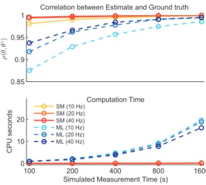
Fig. 1. Comparison between score matching (SM) and max-imum likelihood (ML) estimation for the generalised linear Poisson model. SM achieves high correlation to ground truth (note the y-axis on the upper figure) and approaches the per-formance of ML with considerably lower computational cost.
parameters was quantified using the Pearson correlation coef-ficientρ.
As expected, the ML estimator performed slightly better than the score-matching estimator for small data sizes, partic-ularly for low event rates (Fig. 1). However, correlation co-efficients in both cases were high. With increasing data size both estimators converged to the true solution. The computa-tional cost of the closed-form score matching estimator was over two orders of magnitude lower than the cost of the iter-ative ML estimator, which increases considerably with data size.
ML parameter estimation in practice is often based on binning events at a pre-determined timescale to make esti-mation computationally feasible. If the true intensity func-tion varies more rapidly than the bin-width, such discretisa-tion may mask the true underlying funcdiscretisa-tion. We constructed simulated data as before, but generated the input covariate and events at a sample rate of 5000 Hz, which we binned to 1000 Hz for ML estimation. In our simulations, this mismatch in bin width had a detrimental effect on the fitted parameters (Fig. 2). An advantage of the score matching estimator is that it is evaluated only at the exact event times and does not require any binning. In neural experiments,x(t)is often an experimental stimulus which varies at a fixed rate (for exam-ple, the frame rate of a monitor). Nonetheless, the physio-logical response may be more rapid — for example, with the neurons spiking immediately after a frame refresh rather than uniformly throughout the frame presentation time. Thus, an appropriate choice of bin width may often be unclear.
0.85 0.9 0.95 1
Correlation between Estimate and Ground truth
ρ (ˆ θ , θ ∗) 100 200 400 800 1600 0 10 20 Computation Time CPU seconds
Simulated Measurement Time (s)
SM (10 Hz) SM (20 Hz) SM (40 Hz) ML (10 Hz) ML (20 Hz) ML (40 Hz)
Fig. 2. Comparison between SM and binned ML estimation on the GLM. Binning high-frequency input adversely affects ML estimates. The continuous time SM estimate does not require any binning.
5.2. Generalised Quadratic Model
We then examined the performance of our score-matching estimator for the quadratic (GQM) case, where the log-intensity depended linearly on the outer product of the co-variate function –x(t)x(t)T. Linear weightsθ, now forming a matrix, were chosen randomly; event times simulated; and the resulting estimates ofθevaluated. Maximum likelihood estimation for the GQM is partiularly compuationally burden-some and thus not extensively employed. Instead, we com-pared the score-matching estimator to another closed-form solution that maximises the expected likelihood (MEL) of GQM [9].
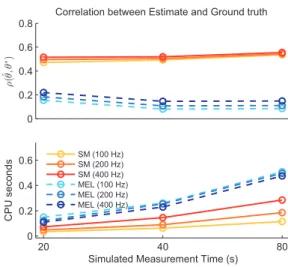
While MEL methods provide a fast and robust way to fit GQM parameters, they rely on the assumption that ex-pected likelihoods can be computed for the given input dis-tribution. If this is the case, as for Gaussian inputs, the MEL estimator’s performance exceeds that of the score matching estimator with only a small increase in computational cost (Fig. 3). However for covariates that follow a more natural non-Gaussian distribution, the MEL estimator is not appro-priate. When events are driven by a covariate based on fil-tered speech waveforms, with the same Gammatone profiles as before, the MEL estimator collapses. The score-matching derivation does not depend on the stimulus distribution, and so is not affected by the change in statistics (Fig. 4). In fact, the estimated parameters are slightly more accurate than with the Gaussian noise covariate, probably because the speech-driven model generates events with greater temporal preci-sion.
0.2 0.4 0.6 0.8 1
Correlation between Estimate and Ground truth
ρ (ˆ θ , θ ∗) 20 40 80 0 0.2 0.4 0.6 0.8 CPU seconds
Simulated Measurement Time (s)
SM (50 Hz) SM (100 Hz) SM (200 Hz) MEL (50 Hz) MEL (100 Hz) MEL (200 Hz)
Fig. 3. Comparison between SM and maximum expected likelihood (MEL) estimation for a generalised quadratic model using Gaussian inputs. MEL offers clear advantages when expected likelihoods are computable with only modest computation burden.
6. CONCLUSION
We have introduced a new class of estimators for point-process models based on measurements in continuous time, and derived specific estimators for “regression” settings where the point-process intensity depends on a known ex-ternal covariate. The estimators are frequently closed-form, and computation scales with the number of events rather than the total interval length. This approach to estimation may help to expand the range of point-process models that can be tractably fit to measured data.
7. REFERENCES
[1] Donald L. Snyder and Michael I. Miller, Random Point Processes in Time and Space, Springer Verlag, New York, second edition, 1991.
[2] Mark Berman and T Rolf Turner, “Approximating point process likelihoods with GLIM,”Appl. Stats., pp. 31–38, 1992.
[3] Aapo Hyv¨arinen, “Estimation of non-normalized statisti-cal models by score matching,”J. Mach. Learn. Res., vol. 6, pp. 695–709, 2005.
[4] Aapo Hyv¨arinen, “Some extensions of score matching,”
Comput. Stats. & Data Anal., vol. 51, no. 5, pp. 2499– 2512, 2007.
[5] Odelia Schwartz, Jonathan W. Pillow, Nicole C. Rust, and
0 0.2 0.4 0.6 0.8
Correlation between Estimate and Ground truth
ρ (ˆ θ , θ ∗) 20 40 80 0 0.2 0.4 0.6 CPU seconds
Simulated Measurement Time (s)
SM (100 Hz) SM (200 Hz) SM (400 Hz) MEL (100 Hz) MEL (200 Hz) MEL (400 Hz)
Fig. 4. Comparison between SM and MEL estimation for a generalised quadratic model using a speech signal input. In-correctly computing expectations based on second order input statistics defeats the MEL approach as expected. SM remains robust (and, indeed, performs slightly better than with Gaus-sian noise).
Eero P. Simoncelli, “Spike-triggered neural characteriza-tion,”J. Vis., vol. 6, no. 4, pp. 484–507, 2006.
[6] Jonathan W. Pillow and Eero P. Simoncelli, “Dimen-sionality reduction in neural models: An information-theoretic generalization of spike-triggered average and covariance analysis,” J. Vis., vol. 6, no. 4, pp. 414–428, 2006.
[7] Tatyana Sharpee, Nicole C. Rust, and William Bialek, “Analyzing neural responses to natural signals: maxi-mally informative dimensions.,”Neural Comput., vol. 16, no. 2, pp. 223–250, 2004.
[8] Ross S. Williamson, Maneesh Sahani, and Jonathan W. Pillow, “The equivalence of information-theoretic and likelihood-based methods for neural dimensionality re-duction,” PLoS Comput. Biol., vol. 11, no. 4, pp. e1004141, 2015.
[9] Il Memming Park, Evan Archer, Nicholas J. Priebe, and Jonathan W. Pillow, “Spectral methods for neu-ral characterization using geneneu-ralized quadratic models.,” inAdvances in Neural Information Processing Systems, vol. 26, pp. 2454–2462. 2013.