Predicting Bank License Revocation

(1)

Worcester Polytechnic Institute

Digital WPI

Interactive Qualifying Projects (All Years) Interactive Qualifying Projects

October 2016

Predicting Bank License Revocation

Everett Jackson Harding

Worcester Polytechnic Institute

Jacob A. Bortell

Michael Joseph Giancola

Parmenion Patias

Follow this and additional works at:https://digitalcommons.wpi.edu/iqp-all

This Unrestricted is brought to you for free and open access by the Interactive Qualifying Projects at Digital WPI. It has been accepted for inclusion in Interactive Qualifying Projects (All Years) by an authorized administrator of Digital WPI. For more information, please [email protected]. Repository Citation

Harding, E. J., Bortell, J. A., Giancola, M. J., & Patias, P. (2016).Predicting Bank License Revocation. Retrieved from

(2)

This report represents work of WPI undergraduate students submitted to the faculty as evidence of a degree requirement. WPI routinely publishes these reports on its web site without editorial or peer review. For more information about the projects program at WPI, see http://www.wpi.edu/Academics/Projects.

Predicting Bank License Revocation

An Interactive Qualifying Project Report Submitted to the Faculty

of the

Worcester Polytechnic Institute

in Partial Fulfillment of the Requirements for the Degree of Bachelor of Science

by:

Jacob Bortell Michael Giancola

Everett Harding Parmenion Patias

Date: 13 October 2016

Report Submitted to:

Professor Thomas J. Balistrieri, Co-Advisor Professor Oleg V. Pavlov, Co-Advisor

(3)

Predicting Bank License Revocation ii

Abstract

The Central Bank of Russia has revoked 20% of all bank licenses since 2012. This project sought to determine a computational method for forecasting the probability of license revocation. To do this, we compared two classification algorithms, logistic regression and random forest. Using a Random Forest classifier produced higher F1 scores than logistic regression. We recommend that Deloitte continues the development of a random forest model by investigating clustering and additional features to improve the model’s performance.

(4)

Predicting Bank License Revocation iii

Acknowledgements

We would like to thank our sponsors at Deloitte for their assistance in completing this project: Dr. Jaroslav Bologov, our main liaison, Dr. Alexey Kozionov, and Dr. Alexey Minin, of the Data Analytics Institute at Deloitte.

We would also like to express our gratitude to our advisors from WPI, Dr. Oleg Pavlov and Dr. Thomas Balistrieri, for their assistance in developing this report and providing us with an enjoyable and intellectually stimulating IQP experience.

Finally, we would like to thank our hosts at the Financial University for their sincere hospitality and warm welcome to Moscow.

(5)

Predicting Bank License Revocation iv

Authorship

The table below indicates the primary contributors to each section of the paper. The contributors are denoted by their initials (JB=Jacob Bortell, MG=Michael Giancola, EH=Everett Harding,

PP=Parmenion Patias)

Section Title Primary Author(s) Primary Editor(s) Abstract JB, MG MG Acknowledgements MG - Authorship PP EH, MG Executive Summary PP MG, EH 1 Introduction PP EH 2 Background - - 2.1 Macroeconomic Conditions PP EH 2.2 Banking Regulations EH PP

2.3 Previous Predictive Models EH

3 Methodology - -

3.1 Build Basic Dataset JB EH

3.2 Develop Basic Models MG EH 3.3 Determine Significant Features MG EH 3.4 Evaluating & Optimizing Model Performance MG EH

4 Results and Findings EH -

4.1 Feature Set EH, PP MG

4.2 Performance of Models EH, PP MG

(8)

Predicting Bank License Revocation vii

6 Conclusion PP EH

Appendix A: Regression Models EH - Appendix B: Random Forest Models EH - Appendix C: Performance Metrics MG EH

Appendix D: Model Code MG -

Appendix E: Parser Code JB -

Appendix F: Glossary PP JB

(9)

Predicting Bank License Revocation viii

Executive Summary

In this project our team compared two models that were created to forecast when the Central Bank of Russia (CBR) may revoke a bank’s license. The models our team used were multinomial logistic regression and random forest. The two models were created and run using the same data in order to compare how they operate and determine which has the best performance.

The data used to develop the models was collected from two databases: Banki.ru and CBR.ru. The data included information found from the financial documents that are published monthly by banks for the CBR and are available to the public. The data included numerical

standards, ratios required by the CBR to decide whether a bank is in an unstable state. Examples of these standards are Current Liquidity and Capital Adequacy Ratio. We created a parsing program to download and update the data collected in order to both save time in this project, but also to provide Deloitte with a tool that can be used in the future.

This data was formatted to form our base dataset. The monthly statistics were sorted into observations. Each observation contained all the statistics reported about a single bank from that month, providing a “snapshot” of the bank’s financial situation. Each observation was also assigned a label that reflected how many months before the bank lost its license the “snapshot” was taken. These labels were: 1 month to 24 months, “Greater than 2 Years”, and “Still Active”. The last of these was used to label observations of banks that still retained their license at the time of our research.

To compare the models, we used three different metrics: precision, recall, and F1. Precision is concerned with the accuracy of the model’s predictions while recall measures the completeness of the predictions. F1 is the harmonic mean of precision and recall.

To optimize the models, the team came up with three alterations that could help identify the best model, as well as differences between the models. The first modification was to preprocess the dataset before passing it to the model. Since the order of magnitude of our data varies greatly from one feature to another, scaling the data can benefit some types of models. Second, we tested the model’s performance on monthly predictions versus quarterly predictions. Finally, we experimented with removing the top 20 and bottom 20 banks by net assets from our dataset. We hypothesized that by removing the banks with extreme values from the dataset, trends in the banks in the middle would become more apparent, improving the performance of both models.

The results of our experiments indicate that the random forest model is better suited for this problem than the regression model. We generated several sets of results to analyze the effects of the optimizations we implemented. Preprocessing improved the regression model slightly, but had negative results on the random forest model. This was understandable, as the benefit of

(10)

Predicting Bank License Revocation ix

method by which regression makes predictions is much more sensitive to the magnitude of features than random forest is. Next, predicting on a quarterly basis produced much higher F1 scores than monthly. The reason is intuitive: the models had more data points per category to base their predictions on. Finally, removing the “extreme” banks had mixed results. It slightly worsened the results of regression, while slightly improving the random forest model. However, the

improvements seen in random forest weren’t large enough to state that the change was responsible for the improvement.

Our team recommends Deloitte to use the random forest model instead of the regression model, and continue with its development. They should check for revocations quarterly, as the predictions are much more accurate than monthly while giving more precise predictions than a yearly analysis. If they need the granularity of a monthly analysis, we suggest they input data which is recorded weekly, as monthly data proved to be insufficient to produce accurate results at that scale. We recommend they do additional research into methods of clustering banks into groups and running the model separately on different clusters.

(11)

Predicting Bank License Revocation 1

1 Introduction

Between 2012 and 2015, the licenses of more than 200 out of 900 banks in the Russian Federation were revoked by the Central Bank of Russia (CBR). (The Moscow Times, 2015) Mr. German Gref, the CEO of one of the largest Russian banks, Sberbank, predicts that another 10% of banks in Russia will lose their licenses by the end of 2016. Bank license revocation affects not only investors, but also commercial and retail clientele who have life savings deposited in these banks. (In Russia, economic recovery remains elusive.2015)

It is difficult to predict when the CBR will revoke a bank’s license due to the wide array of circumstances that can lead to a license revocation. Failure of banks to meet the required standards set in the banking legislation is a sure condition for the CBR to revoke a bank’s license.

Additionally, the CBR can revoke a bank’s license if they have substantial proof that fraud has taken place, if the bank has conducted operations not covered by the bank's license, or based on 20 other cases included in Federal Law 395-8, Article 20. (On Banks and Banking Activities, 1990)

Predictive models have been developed to forecast the probability of a bank going bankrupt. Researchers have used different methods, including regression models and neural networks to achieve accuracy level upward of 80%. (Boyacioglu, Kara, & Baykan, 2009) Some papers have provided analysis of the factors included in the model. For example, Mayes and Stremmel (2012) found that “the non-risk-weighted capital measure explains bank distress and failures best.” (Khalafalla Ahmed Mohamed Arabi, 2013) Due to the instability of the economy in past years, an accurate model to forecast the closure of banks can provide consumers and investors with a way to confirm that their money will be safe with a particular bank.

The goal of this project was to generate a model capable of accurately forecasting when a bank’s license will be revoked by the CBR. To expand upon previous work, we developed and compared two multinomial classification models which would forecast up to two years in the future when a bank may lose its license. The models’ performances were verified using several methods of performance analysis. Finally, one of the models was selected as a recommendation for continued research.

(12)

2 Background

2.1 Macroeconomic Conditions

Banks in Russia are in the midst of several challenges, including economic sanctions that prevent foreign investments and the decline of oil prices starting in 2014. After the drop of the price of oil in 2008, it became clear that Russia’s economy was based on two staples which are heavily connected: oil and hedge fund investments. Every time one of the two undergoes a crisis the second follows, due to the high investments of hedge funds in oil (The Economist, Issue 8985, 2016). Currently, increasing the oil price is a matter of great importance for the Russians. This concern was reflected in the first day of the 2016 G20 Summit in China, when the President of Russia (and the Crown Prince of Saudi Arabia) commented on the need to discuss oil prices (Workman, 2016).

Given the probability of an oil crisis the Kremlin has promoted a diversification of

investing, focusing on exporting non-petroleum products (such as metal). At the same time the CBR has increased Russia’s international reserves from 140Bn USD to 500Bn USD, during the 2009-2013 period, while allowing the Russian Ruble to float (The Economist, Issue 8985, 2016). Instead of spending all the reserves on keeping the value of the Russian Ruble on par with the dollar, they concentrated on helping institutions affected by the economic sanctions imposed by the European Union and the United States. This shift of focus from defense of the Russian Ruble to support of domestic institutions resulted in a 10% decrease in the actual salary of Russians (inflation

fluctuation). However, it bears mention that the average Russian’s salary remains triple the size it was before Mr. Putin became President, which shows a general upward trend since the 1998 crisis.

From 2014 to 2016 Russia’s currency depreciated from 35 Russian Rubles to 1 USD to 64 to 1. The Kremlin put its trust in Mr. Elvira Nabiullina as the new head of the Central Bank of Russia (CBR) in 2013 (Reuters.com, 2016). Since her instatement at the head of the CBR, the organization has rapidly revoked the licenses of more than 200 financial institutions (Weaver, 2015). The motive behind the revocations has been debated. Ms. Nabiullina “received carte blanche

from the president to go after those banks that were earlier untouchable,” says Mr. Oleg Vyugin, chairman of MDM Bank and a former deputy governor of the Central Bank. Ms. Nabiullina stated “This [revoking of licenses] is not a cleansing effort. This is an effort to make the banking sector viable and get rid of the weak players”.

Russian Banks are usually divided in three categories by specialists. The top tier, which can be thought of as “too strong to fail,” can be considered almost certain to keep their license. The second tier, the top 100 banks, is comprised of those institutions expected to survive the worst of crises but with less certainty. The third tier contains the remaining banks, institutions of varying stability which are trying to survive and maintain their licenses. However, a good ranking does not

(13)

Predicting Bank License Revocation 3 guarantee a bank’s survival. Despite its position as one of the “Top 100” banks, Master Bank’s license was revoked in 2013.

The CBR revoked the Master Bank’s license based on money-laundering violations and suspicious transactions. The bank had a 2 Bn USD hole in its balance sheet, owed almost 1 Bn USD’s to its depositors, and disrupted the operations of numerous other banks (Makhonin, 2013). Russia’s banking system has been hit many times by these kinds of illegal activities and the stock market is still seen by many as a money laundering paradise. The problematic state of the banks can be seen again through some extreme examples of banks’ illegal activities. According to the CBR, Admiralteisky Bank’s license was revoked due to “inability to follow anti-laundering rules and because it practically stopped serving its clients.” Moreover, when CBR officials opened the bank’s vaults, they found iron bars painted gold, evidence of a bank falsifying its assets (Amos, 2015).

Between the years 2008 and 2013 the CBR revoked, on average, 30 licenses per year. This number was almost tripled in 2014 when more than 80 licenses were revoked (Weaver, 2015). The uptick in revocations shows that Russia has decided it needs to rely on more than its size and its oil in order to keep its position as one of the strongest countries. Strengthening the economy is one important step. To be certain of this strength Russia needs to make sure that no bank will unexpectedly reach a point where its license will need to be revoked, possibly leading to events similar to the events of 2008 in the United States. To reach such a state of certainty it needs strong, law-abiding banks.

2.2 Banking Regulation

Banking regulation refers to the laws that banks must follow to legally operate in the Russian Federation. The regulations are set by the Central Bank of Russia (CBR). The regulation outlines the criteria and process for evaluating the performance of each bank. A key component of these regulations are the banking normatives, a set of numerical standards that regulate the levels to which a bank can take risks. These standards are defined in Federal Law No. 87 FZ, Article 62. Those below are outlined in Bank of Russia Instruction No. 139-I:

1) Capital Adequacy (N1) The minimum allowable value for this ratio is 10%.

a) Capital Adequacy ratio (N1.0) Capital adequacy ratios make sure that banks have enough capital to absorb losses without going bankrupt. Each ratio governs different components of a bank’s capital. N1.0 regulates the entirety of a bank’s capital. The minimum allowable value for this ratio is 8%. b) Common Capital Adequacy ratio (N1.1) This is a ratio of a bank’s equity

capital combined with its disclosed reserves to its risk-weighted assets. The minimum allowable value for this ratio is 4.5%.

(14)

Predicting Bank License Revocation 4 c) Tier 1 Capital Adequacy ratio (N1.2) This expands on the Common Capital

adequacy ratio, including some forms of preferred and common stock with the equity capital. The minimum allowable value for this ratio is 6% 2) Liquidity

a) Quick bank liquidity ratio (N2) - Regulates possible liquidation losses in the next business day. Calculated minimum ratio of high-liquidity assets to on-call obligations must be at least 15%

b) Current bank liquidity ratio (N3) - Regulates the risk of liquidation losses in the 30 days after its calculation. It is the ratio of the bank’s liquid assets to its liabilities due within the regulation time period. The minimum allowable value for this ratio is 50%.

c) Long-term bank liquidity ratio (N4) - Regulates the risk of banks losing liquidity to long-term investments. It is the ratio of a bank’s credit claims maturing after the next 365 days from the date of calculation to the sum of bank’s equity and liabilities that will mature in the same timeframe. This is also adjusted for liabilities of the bank maturing within the next 365 days. This ratio can be at most 120%. In other words, the long-term fiscal stability of the bank cannot be wholly dependent on money the bank does not yet possess.

3) Maximum Risk per borrower or group of borrowers (N6) - Regulates the credit risk of a bank in relation to one borrower or group of borrowers. It is calculated as the ratio of the total credit claims the bank has against a borrower to the bank’s equity. There are some cases for which N6 is not calculated, such as when the borrower is the Russian Federation, federal executive bodies, or the CBR. It is also not

calculated for borrowers that are also stakeholders of the firm (these are covered by N9 and N10). The maximum value for this ratio is 25%.

4) Maximum value of major credit risk (N7) - Regulates the maximum total value of the major credit risks of an institution. It is calculated as the ratio of the major credit risks to the bank’s equity. The maximum value for this ratio is 800%. This large value allows the major credit risks to exceed the capital of the bank up to 8 times in a year.

5) Maximum value of loans, guarantees, and sureties issued by the bank to shareholders (N9.1) - Regulates credit risk on a bank in relation to its shareholders. Calculated as the ratio of the total loans, sureties, and guarantees issued by the bank to its

shareholders to the bank’s equity. The maximum value for this ratio is set at 50%. 6) Total risk on bank insiders (N10.1) - Regulates the amount of risk the bank can have

on anyone able to influence the decision to issue a loan to (place risk on) someone. This ratio is calculated as the total credit risks and financial derivatives that the bank

(15)

Predicting Bank License Revocation 5 has with everyone able to influence the decision to go ahead with those kind of transactions to the bank’s equity. This ratios maximum value is set at 3%.

7) Use of equity to purchase shares of other legal entities (N12) - Regulates the amount of a bank’s equity that can be used to purchase shares of other legal entities. The maximum value of this ratio is set at 25%.

2.3 Previous Prediction Models

A paper examining bankruptcy in Taiwan of examined the effectiveness and predictive accuracy of multiple discriminant analysis, logit regression, probit regression and Artificial Neural Networks (ANN) techniques (Lin, 2009). This study used univariate logistic regression to select which financial ratios to use as variables in the development of each of the four models above. The selection narrowed 44 ratios considered to 20 ratios used in the study. By narrowing the focus of the model, the study was able to eliminate factors that had no effect on the dependent variable. If

included in the model, these factors would only add noise to the data, detracting from the accuracy of the model.

A model developed in 2006 compared the accuracy of logit regression and trait recognition models (models that look for approximate patterns in a dataset and can make predictions on data points that are not exact matches to the trend) (Lanine & Vennet, 2006). The paper predicted bank failures in the Russian sector quarterly, in periods of 3 months, 6 months, 9 months, and 12 months. In this application, the models showed that liquidity of bank assets to be an important determinant of bank license revocation predictions. It also cites asset quality and capital adequacy as significant determinants. Other factors used in the models developed in the paper are return on assets (ratio of net income: total assets), government debts securities (ratio of government debts: total assets), overdue loans (ratio of overdue loans + overdue promissory notes: total loans), ratio of loans to total assets, and a value for the size of the bank calculated as Log(total assets) (Lanine & Vennet, 2006).

Another model, aimed specifically at predicting defaults in the Russian banking sector in the timeframe 1997-2003, explored the benefits of clustering banks into groups of comparable banks, then developing individual models for each cluster. The study separated banks in four ways: by the ratio of their investments in government bonds to their total assets, the size of the bank’s assets relative to the total market assets, the ratio of banks credits-to-non-financial firms to total assets, and the ratio of the bank’s equity to its total assets. This paper clustered each bank into three categories based on “small”, “medium”, and “large” values of each of these four parameters. After clustering, the paper found the liquidity, equity and government investments to be significant indicators of a bank’s eventual default/avoidance of default (Peresetsky, Karminsky, & Golovan, 2011).

(16)

Predicting Bank License Revocation 6 The findings of these papers indicate that the significant factors in predicting defaults (license revocations) of banks can be seen in the capital adequacy or equity ratio (defined as N1 by the CBR) and liquidity ratios (defined as N2 through N4 by the CBR). Given the significance of these factors determined by the CBR and third parties, our model development will begin with the inclusion of the normatives N1, N2, and N3.

3 Methodology

The goal of this project was to forecast when a bank is likely to have its license revoked by the CBR. Previous papers have framed the problem of forecasting bank license revocations as a binary situation (revoked/not revoked). Our approach attempts to forecast the time until a bank will lose its license. We created a pair of models with this in mind. Provisions are made in the

development of both models for the case where a bank does not lose its license.

The first of the models we used was a multinomial logistic regression model. This model is a statistical method that takes the logistic regression algorithm used as a baseline in previous works and extends it to forecast months rather than whether or not the license was revoked. For simplicity, we refer to this model as our “regression” model. This regression model produces a set of equations that estimate the number of months until a bank loses its license. For further details on the

implementation of regression models, see Appendix A.

The second of the models we used was a random forest model. This is a machine learning method that has not to our knowledge been used in this application. Like the regression model, the random forest attempts to forecast the date a bank’s license is revoked. Instead of an equation, a random forest produces a set of decision trees to forecast the number of months until a bank loses its license. For more information on random forest models see Appendix B.

The objectives and corresponding methods for the development of these models are summarized in Table 3.

(17)

Table 3: Objectives and Methods

Objectives Methods

1. Collect financial data into base dataset ● Create a script to draw data from online

databases

● Organize data into a manageable form 2. Determine the significant financial factors

which indicate a propensity for license revocation

● Evaluate the relevance of each available factor ● Graph factors over revocation status to find

trends

3. Develop the models ● Discuss with Deloitte liaisons the best practices

for creating effective models using financial data

● Use the Python library scikit-learn

4. Analyze and compare performance of models ● Apply Precision, Recall & F1 metrics

● Generate optimal models for comparison with

each other

3.1 First Objective: Build Basic Dataset

We downloaded our data from two online databases: banki.ru and the Central Bank of

Russia’s (CBR) public records. The first database, banki.ru, contains 89 monthly statistics on each financial institution in the Russian Federation dating back to March 2008. It also contains a list of license revocation dates for banks that are no longer operational. The CBR database contains bank statistics reported monthly in compliance with the standards described in Chapter 2.2 of our report. After downloading data from both sources, we used it to generate our dataset for the development of the models.

It should be noted that each observation in the dataset is independent of a specific license number. Before being put into the model, the license numbers are removed, so each observation becomes a different picture of the same nameless bank. The problem is not to find trends that lead banks to fail over time, but to find sets of values that correspond to banks that are (x) months or quarters from failure.

This combination was done in two steps. First, we combined the data from banki.ru with the data from CBR to create a set of monthly observations. Each of these observations provides a

(18)

Predicting Bank License Revocation 8 snapshot of the financial situation of a bank at the beginning of the month. This observation of a bank is a collection of the monthly statistics about that bank. Each of these statistics is called a

feature of the observation. Initially we used only three statistics, N1, N2, and N3, as features of the observations. More banking statistics were added as features later.

Second, we classified each of the observations from the first step by the number of months between the date of that observation and the date the bank eventually lost its license. If this number was greater than 24, we assigned the observation a special value of 1000 to signify that it

represented the bank’s financial situation more than two years before the bank’s license was

revoked. If an observation is of a bank that has not yet lost its license, it is assigned a value of 9000, signifying that there is no revocation date for that bank. The final combination of our observations and their classifications formed our dataset. For more details on the downloading and combination of our data, see the Python code in Appendix E.

We split our dataset into two similar parts for model development. Each part had the same proportion of observations from each class. Creating the sets in this way is called stratifying the two sets. The first set, called the training set, was used to build the models. The second set, called the testing set, was used to evaluate the performance of the models.

Finally, we added one more component to our observations before inserting them to the models. For various reasons, the value of some statistics may be missing for a bank in a particular month. However, the model cannot run on incomplete data. To handle not-reported data, we set the value of the missing feature to 0, and add a new feature called X_M?, where X is the name of the feature with the missing value. This feature is given the value 0 when the corresponding feature has no value, and 1 when the feature has a value.

3.2 Second Objective: Develop Basic Models

In completion of this objective we built simple versions of each model (Logistic Regression

and Random Forest) which were later improved and compared. We developed the models using the

scikit-learn library for Python. Scikit-learn is a machine learning library designed to aid developers in data analysis. It has functions to create classification models, implement clustering algorithms, and a variety of related operations. We used the classification functions to build our model because they best fit the way we structured the dataset.

Both models were built with the same training set. Each model is created by an algorithm that looks for trends in the observations that correlate to the classes (number of months until license revocation) assigned to the observations. This process of building the model based on the training data is called fitting the model. After the first fitting of the models, we repeated the process in our first objective to include more statistics as features in the observations.

(19)

3.3 Third Objective: Determine Significant Features

We determined which of the available banking statistics were significant as features of our observations for the two methods: one for the regression model and one for the random forest model. The random forest determines internally which features of the observations are significant (Fawagreh, Gaber, & Elyan, 2014). To determine which features were significant in the regression model we used a method of combining the emphasis placed on that feature with its standard deviation in the dataset (Peresetsky, Karminsky, & Golovan, 2011). This method is described further in Appendix A.

We compared the two determinations and selected the features of greatest significance as the features to include in the next iteration of the model. Having selected our significant features, we repeated the processes of generating our dataset, splitting it into the two stratified sets (training and testing), and fitting the model to the training set.

3.4 Fourth Objective: Evaluating & Optimizing Model Performance

3.4.1 Evaluating Model Performance

After fitting our models and selecting the significant features, we used the testing set from our first objective to determine how well the models could forecast the date a bank would lose its license. We input the observations from the testing set into the models, which output the estimated classification of each observation. We compared these estimated classifications with the actual classifications using three different evaluation metrics.

The first of these metrics is called precision. This is a measure of how correct each model’s estimations were. It answers the question “how many observations did the model classify

correctly?” The second of these metrics is called recall. This is a measure of how complete each model’s estimations were. It answers the question “how many observations of this classification did the model identify?” The third metric is a combination of the first two called F1. It provides an answer to the general question “how well did the model perform?” Details on the calculation of each metric can be found in Appendix C.

3.4.2 Optimizing Model Performance

The goal of optimizing model performance is to achieve the highest scores possible in each of our evaluation metrics. To maximize our model’s scores, we made three edits to the original models.

First, we added a step to the dataset creation called preprocessing. Preprocessing is a

(20)

Figure 1: Percentage of data in each class,

“1 Quarter Left” to “Still Active” values that range from thousands in some observations to billions in other observations.

Preprocessing transforms all the values of this feature into values within a much more manageable range. This is intended to minimize the impact of the discrepancy between magnitudes of the values.

Second, we changed the way we classified our observations. Instead of classifying each observation by how many months it was from the date of the bank’s license revocation, we

classified each observation by how many business quarters it was from the date that bank’s license was revoked. By changing the classifications we hoped to increase the resolution of our data, as there would be multiple observations of each bank in each classification.

Third, we removed the extreme observations from the dataset. We elected to remove all observations of the 20 largest and 20 smallest banks as reported by net assets. By excluding the extremes we hoped to remove anomalies from the data that would skew the results of the model.

4 Results & Findings

Before analyzing our results, we must discuss the composition of our dataset, as it has a significant effect on the results of our models. Despite the increase in bank license revocations, there are many more banks that are still active than there are banks that have lost their license. Because each of these banks are still

active, they continue to produce new statistics each month, while the banks whose license has been revoked no longer produce new statistics. Therefore, as shown in Figure 1, we have much more data about the banks that are still active than we have about the banks that have lost their license. To further compound the bias, all observations of the “still active” banks (76% of the dataset) are in one class, while the data about banks that have lost their license (24% of the dataset) was further divided into 9 classes.

More than half of the data that reflects banks whose licenses have been revoked (14% of the total dataset) is contained in the “Greater than 2 Years Left,” leaving only 10% of the dataset to be divided among the remaining eight classes.

(21)

Predicting Bank License Revocation 11 With such a significant bias in the dataset, the models are provided with much higher amount of information in the “Still Active” class than the “> 2 years” and quarterly classes, which allows a better estimate of what constitutes a “Still Active” bank than the estimates of the lower classes.

4.1 Performance of Models

Since F1 is determined by both the precision and recall score, it is an appropriate metric to compare models. However, for additional insight into the performance of the model, we will consider the specific precision and recall scores individually.

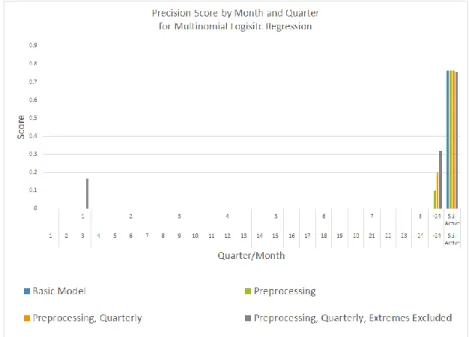
4.1.1 Multinomial Logistic Regression

(22)

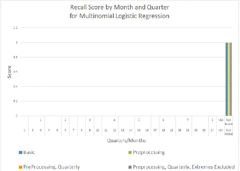
Figure 3: Recall scores for each iteration of our regression model

Figure 4: F1 scores for our regression model.

From Figures 2, 3, and 4 we can see that our regression model produces results with next to zero scores in most classes for all three metrics. The precision scores show the most success, with ~15% in the one quarter to revocation (for its best version) and between 10% and 30% in the > 2 years until revocation class for all versions but the basic version. All metrics show very high performance in the “Still Active” class. The recall score in this class is 100%, but the precision in

(23)

Predicting Bank License Revocation 13 this class is only ~75%, which indicates the model defaults to guessing that an observation belongs in the “Still Active” class, likely due to the bias in the dataset described above.

4.1.2 Random Forest Model

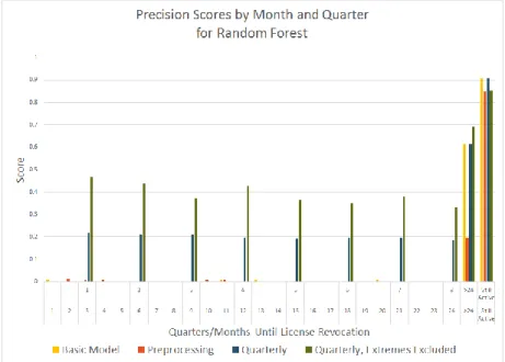
Figure 5: Precision scores for each iteration of our random forest model

(24)

Figure 7: F1 scores for each iteration of our random forest model.

As we can see from Figures 5, 6, and 7 the random forest model was not improved by adding preprocessing, although it performs much better when run quarterly (as opposed to monthly). Generally, the quarterly model with extreme banks excluded (the top and bottom 20 banks by net assets) scores highest by F1, however it is too close to be statistically significant.

Achieving an over 20% average score between Q1-Q8 is a positive result. The model’s precision and recall were similar for all iterations except the “Quarterly, Extremes Excluded”. As illustrated in Figure 8, the precision score for this iteration was much higher (between 35%-45%) than the recall (around 10%).

(25)

Figure 8: All metrics for best performing random forest model, calculate quarterly with the top 20 and bottom 20 (by net assets) banks excluded

We compared the “Quarterly, Extremes Excluded” model to the results of randomly guessing which observation from our testing set belonged to which category. The distribution our guesses matched the distribution of the dataset, meaning 76% of our guesses were that an

observation belonged to the “Still Active” class, 14% in the “> 2 years” class, etc. When applying our performance metrics to our random guesses, we found that the random forest model

(26)

Figure 8: F1 scores for random forest model graphed next to F1 scores for random guessing

(27)

4.1.3 Model Comparison

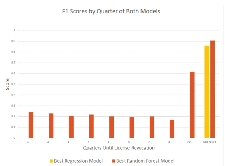
Figure 9: Comparison of best regression and best random forest model

Figure 9 shows the comparison of the optimal regression and random forest models. As discussed previously, regression only performs better than randomly guessing in one class, so clearly the random forest model is our best model. Our random forest model scores in the 15-25% range for the first 8 classes, scoring over 60% in the 9th and over 90% in the 10th class.

4.2 Significant Feature Set

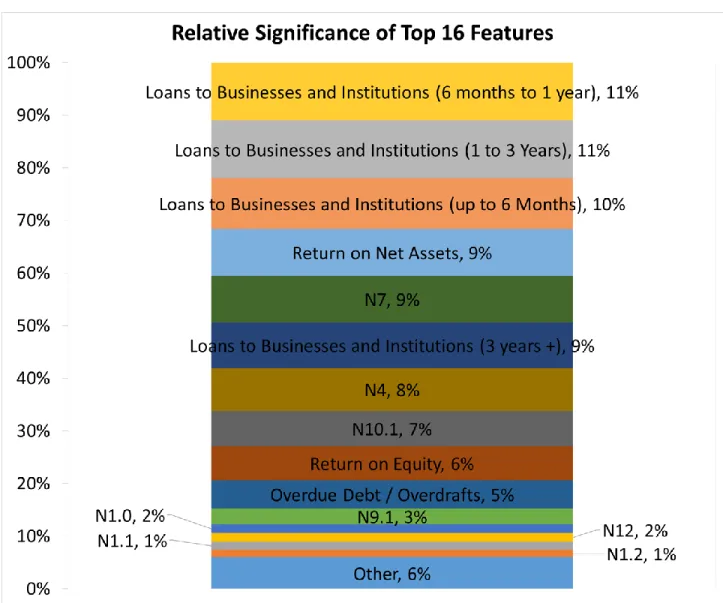
The feature set used to generate our results is shown in Appendix G. Feature significance was determined for the random forest model using the Gini Importance (G.I.), which is the mean of the Gini Impurity Index1_{of each feature determined by all the decision trees in the random forest.}

For simplicity’s sake it can be thought of as a “Percent Weight”, or a percentage of the model’s

(28)

Predicting Bank License Revocation 18 prediction determined by that feature. The percent weights are shown in Figure 10 for each of the top 16 most-significant features. These features comprise 94% of the random forest’s consideration. The other 31 features make up only 6% of the consideration of the model.

Figure 10 shows that the most significant factor is the total of all loans extended to

institutions and businesses to be repaid in a three year period. Loans are directly involved with risk, thus we can speculate that the CBR pays attention to the investing of different banks and tries to keep them safe in and stable levels. By revoking licenses of banks that take too much risk, the CBR strengthens the economy by lowering the probability of these credit institutions going bankrupt and snowballing others with them.

Figure 10 also shows that the features indicating whether or not a value was reported are entirely contained in the “other” features, as none of them appear in the “Top 16”. The nature of the approach of the random forest model makes this type of feature redundant. However, for

(29)

Predicting Bank License Revocation 19 consistency in the comparison of the models, they were included for the random forest model because they were necessary in the logistic regression.

We expected N2 and N3 to be two of the most significant features but the random forest model calculated their significance as 25th and 21st respectively. Despite their use by the CBR, these ratios were shown to be insignificant in the random forest model. They were indicated as the two values with the greatest significance in the logistic regression model, but as that model did not yield a high performance, we cannot confirm the validity of this significance. The standards considered significant (greater than 1% of the consideration) were N9.1, N1.0, N12, N1.1, and N1.2.

5 Recommendations

5.1 Use Random Forest

Our results have shown that, for this application, the random forest algorithm scores higher on precision, recall, and F1 than the logistic regression algorithm. Specifically, it scores higher in all classes of the target variable. Therefore, we recommend that Deloitte continues to pursue the random forest approach rather than the multinomial logistic regression.

5.2 Predict on Broader Timeframes

We recommend Deloitte build models that predict on a quarterly basis, as both random forest and regression performed better under fewer target variable values. One likely cause of this is that our data is recorded every month. Predicting into quarters instead of months gives each class of target variable more observations, and a higher likelihood the model will find trends. Another option to improve model performance is to predict over even broader timeframes. For example, we ran our model on 4 classes, revocation in 1 year, 2 years, more than 2 years, or never, and got F1 scores of 43%, 41%, 63%, and 91% respectively. Those scores are generally higher than their respective counterparts in the quarterly model, although the predictions provided by this model are less precise.

5.3 Identify More Significant Features

We also recommend that Deloitte use more of the available data. One statistic in particular that we recommend Deloitte investigate is the ratio of precious metals over net assets. The precious metals data can be found from CBR’s form 110. The past years there has been a global shift from USD reserves to Gold reserves, thus the amount of gold reserves in a bank could indicate said bank’s importance for the Russian economy. Deloitte should also test additional data related to

(30)

loans and risk evaluation. Based on results from both models, the features with most significance were the ones related to risk or loans. This is probably because the CBR tries to stop any over-risky investment, due to the probability bankruptcy.

5.4 Consider Effect of Preprocessing Data

Preprocessing the data before running the regression and the random forest models produced different results in each model. Preprocessing improved performance in the metrics for our

regression model, but worsened results for Random Forest. This was expected, as the benefit of preprocessing is dependent on the way the models interpret the training data.

Regression develops an equation that combines the numerical values of each feature in the observations. Therefore, it is possible that the importance of some features might be skewed if they have a large variance in their values (some values between 0 and 1 and others in millions).

Random Forests internally divide all values of each feature into ranges during their development. Preprocessing reduces the resolution of those ranges, so we see a slight drop in performance values. Therefore we recommend Deloitte avoid using preprocessing if they continue to develop the random forest model.

5.5 Improvements Using Geopolitical Features

In addition to economic considerations, there are geopolitical and sociological factors that can lead to bank license revocation. We recommend, to further improve our model, that Deloitte add additional algorithms that analyze the current geopolitical and sociological environment and study how it influences banks. An example for such an implication would be to search how often a bank in referred to in the news, in a positive or negative way, and how this affects the bank.

5.6 Removing Extreme Banks

We ran both models with and without data from the top 20 and bottom 20 banks by net assets. We found that these banks, due to their size, behave differently than most banks. We hypothesized that removing them may make trends in most banks more clear, leading to improved results. We saw slight improvements in the random forest model using this method, however the improvements weren’t significant enough to fully recommend this practice.

However, we would recommend that Deloitte investigate the effect of removing banks from the dataset which had their licenses revoked due to non-economic reasons (eg. fraud). Banks that lost their licenses due to illicit activities likely don’t follow the same patterns as banks which lost their license due to economic failure, so removing these banks should make trends in the other banks more clear.

(31)

5.7 Use Clustering

Finally, we recommend Deloitte cluster the banks in the dataset. By clustering, we mean to group the banks based on a specific characteristic and generate a separate model each cluster. For example, instead of removing the extreme banks by net assets, Deloitte could cluster the banks into the top 10%, middle 80%, and bottom 10% by net assets, then run the model separately on each cluster. The idea is that banks within a cluster follow trends that are unique to banks in that cluster, but are obfuscated by observations outside the cluster in the general dataset. Therefore, clustering makes these individual trends clearer, resulting in improved performance in each cluster as opposed to running the model once on all banks.

6 Conclusion

Our research shows that a model using random forest scores higher on precision, recall, and F1 than one using multinomial logistic regression when used to forecast revocation of Russian bank licenses. We found that both models perform better when predicting quarters of the year instead of months. Also, our regression model is improved by preprocessing, while the performance of our random forest model worsens. The effect of excluding the top 20 and bottom 20 banks by net assets is negligible, although it improved the random forest model slightly.

To continue our work, Deloitte could research and add additional features for the Random Forest model. We found that adding features generally improves model performance. Specifically, the model would be improved by data that is recorded more frequently (eg. per week) than the data currently available, which is only updated every month. This made predicting failure on a monthly basis nearly impossible, but was sufficient for a quarterly analysis. Finally, Deloitte could

investigate clustering the banks based on certain characteristics (eg. net assets, loans to businesses) and running the model on individual clusters separately. There may be trends in the data which exist only in certain clusters; separating banks in this way would help the model recognize these trends and improve model performance.

(32)

References

Amos, H. (2015). Russia's biggest banking crashes of the last 2 years. Retrieved from

https://themoscowtimes.com/articles/russias-biggest-banking-crashes-of-the-last-2-years-49505

Boyacioglu, M. A., Kara, Y., & Baykan, Ö K. (2009). Predicting bank financial failures using neural networks, support vector machines and multivariate statistical methods: A comparative analysis in the sample of savings deposit insurance fund (SDIF) transferred banks in turkey.

Expert Systems with Applications, 36(2), 3355-3366. doi:10.1016/j.eswa.2008.01.003

Breiman, L. (2001). Random forests. Machine Learning, 45(1), 5-32. Doi:1010933404324

Capstone. (2003). The capstone encyclopaedia of business (1st ed.). GB: Capstone Publishing Ltd. Retrieved from http://replace-me/ebraryid=10788037

Fabozzi, F. J., Focardi, S. M., & Rachev, S. T. (2014). Basics of financial econometrics. Somerset, US: Wiley. Retrieved from http://site.ebrary.com/lib/alltitles/docDetail.action?docID=10845560 Fawagreh, K., Gaber, M. M., & Elyan, E. (2014). Random forests: From early developments to

recent advancements. Systems Science & Control Engineering, 2(1), 602-609. doi:10.1080/21642583.2014.956265

Greene, W. H. (2003). Econometric analysis (5. ed.). Upper Saddle River, NJ: Prentice Hall. In Russia, economic recovery remains elusive. (2015). Stratfor, Retrieved from

https://www.stratfor.com/analysis/russia-economic-recovery-remains-elusive

Karminsky, A., & Kostrov, A. (2014). Comparison of bank financial stability factors in CIS countries. Procedia Computer Science, 31, 766-772. doi:10.1016/j.procs.2014.05.326 Kerr, A., Ngondi, G. E., & Butterfield, A. (2016). A dictionary of computer science Oxford

University Press. Retrieved from

http://www.vlebooks.com/vleweb/product/openreader?id=none&isbn=9780191002885&uid=non e

Khalafalla Ahmed Mohamed Arabi. (2013). Predicting banks' failure: The case of banking sector in Sudan for the period (2002-2009). Journal of Business Studies Quarterly, 4(3), 160. Retrieved from http://search.proquest.com/docview/1476893509

Lanine, G., & Vennet, R. V. (2006). Failure prediction in the Russian bank sector with logit and trait recognition models. Expert Systems with Applications, 30(3), 463-478.

(33)

Predicting Bank License Revocation 23 Liaw, A., & Wiener, M. (2002). Classification and regression from random forest. R News, 2/3,

18-27. Retrieved from

ftp://131.252.97.79/Transfer/Treg/WFRE_Articles/Liaw_02_Classification%20and%20regressio n%20by%20randomForest.pdf

Lin, T. (2009). A cross model study of corporate financial distress prediction in Taiwan: Multiple discriminant analysis, logit, probit and neural networks models. Neurocomputing, 72(16–18), 3507-3516. doi:10.1016/j.neucom.2009.02.018

Makhonin, A. (2013). $1Bln owed to depositors as master bank has license revoked. Retrieved from

https://themoscowtimes.com/articles/1bln-owed-to-depositors-as-master-bank-has-license-revoked-29777

Mitchell, T. M. (1997). Chapter 3: Decision tree learning. Machine learning (pp. 52-77) McGraw-Hill.

On banks and banking activities, Federal LawU.S.C. (1990). On statutory ratios for banks, InstructionU.S.C. (2012).

Peresetsky, A., Karminsky, A., & Golovan, S. (2011). Probability of default models of Russian banks. Economic Change and Restructuring, 44(4), 297-334. doi:10.1007/s10644-011-9103-2 Putin's right-hand woman; Russia's central-bank governor. (2016). The Economist, 419(8985), 60. The Moscow Times. (2015). 500 Russian banks to close within 5 years, VTB head says. Retrieved

from https://themoscowtimes.com/articles/500-russian-banks-to-close-within-5-years-vtb-head-says-47965

Weaver, C. (2015). Russia’s anatoly motylyov: Rise, fall, repeat - FT.com. Retrieved from

http://www.ft.com/cms/s/0/4eecb666-52eb-11e5-b029-b9d50a74fd14.html

Workman, D. (2016). Crude oil exports by country. Retrieved from

(34)

Appendix A: Regression Models

Running regression analysis on a set of data yields an equation that estimates the outcome of an unknown statistical event. It finds application in a variety of financial analysis techniques and models in various forms. The most common of forms of regression are linear, probit, and logit regression. Regression can be categorized by the number of independent variables considered. These categories are univariate (one independent variable) and multivariate (multiple independent variables). The regression models used for forecasting bank failures are generally the latter

(Fabozzi, Focardi, & Rachev, 2014; Greene, 2003).

The most basic regression technique, linear regression, describes the trend in a data set with the assumption that any trends will be linear in nature. In univariate regression, this will yield a “line of best fit” for the data. In multiple regression, the output will be a series of coefficients that describe a hyperplane. This hyperplane is analogous to the “line of best fit” seen in univariate analyses, as it provides an estimation of the general trend of the dataset. The general form of the linear regression model is:

𝑦 = 𝛽₀+ 𝛽₁𝑥₁+ ⋯ + 𝛽_𝑘𝑥_𝑘+ 𝜖 (1)

where y is the dependent variable and xi is a component of vector x. The error term is

included to account for the inherent inaccuracy in the approximation of the model (Greene, 2003). The second technique, probit regression, provides a non-linear analysis of a set of data. It gives as an output the probability of a binary event, with predictive values between 0 and 1. This method takes the general form:

𝑃(𝑦|𝑋₁, 𝑋₂, … , 𝑋_𝑛) = 𝑁(𝛽₀+ 𝛽₁𝑥₁+ ⋯ + 𝛽_𝑘𝑥_𝑘) (2)

where N means the error term takes the cumulative normal standard distribution function. In essence this means the variables are inserted, transformed by the coefficients, and then the

probability of failure is calculated based on an assumed probability density curve (Fabozzi, Focardi, & Rachev, 2014).

The logit regression model is similar but it assumes that the error term takes a different probability density function than probit regression. For the logit model, it is assumed the data takes a logistic probability form, so its general form becomes:

𝑃(𝑦|𝑋₁, 𝑋₂, … 𝑋_𝑛) = 𝐹(𝛽₀+ 𝛽₁𝑥₁+ ⋯ 𝛽_𝑘𝑥_𝑘) (3)

where F represents the error term taking a logistic distribution. With a little algebra, this becomes:

𝑃(𝑦|𝑋₁, 𝑋₂, … , 𝑋_𝑛) = 1

(35)

Predicting Bank License Revocation 25 (Fabozzi et al., 2014) Logit regression has been found to work best in some cases of estimating the probabilities of defaults in banks (Karminsky & Kostrov, 2014).

Another regression model often used in the literature is binary logistic regression, which takes the general form:

log_1−𝑥𝑥𝑎𝑣𝑔

𝑎𝑣𝑔= 𝛽0+ 𝛽1𝑥1+ ⋯ + 𝛽𝑘𝑥𝑘 (5)

where xavg is the mean value of x. The left side is the log of the odds function of xavg. The

log of the odds function is also called the logit function, expressed as logit(xavg). The right side is

the linear combination of x as a vector of k regressors. When used in binary logistic regression, the value of the left side of the equation can be described as the logit(π) (Greene, 2003).

Binary logistic regression models show how a binary dependent variable (in this case the revocation/continuation of a bank license) depends on a set of independent variables x1...xk (in this

case the collection of normatives and indicators selected). The application of the regression allows the calculation of the weight of factors involved in the probability of default (PD) of a bank (Karminsky & Kostrov, 2014). In the application of the probability of default, these factors are selected ratios that compare capitalization and liquidity of banks. When the regression is run, it returns values of the coefficients of the ratios used in the model. The values of these coefficients indicate the effect that each ratio will have on whether or not the bank experiences a default.

Regression models are rarely, if ever, computed by hand. Instead, scripts are written in code. The scripts take in large sets of empirical data, and use those data points to estimate values for each coefficient in the model (Greene, 2003).

(36)

Appendix B: Random Forests

Random forests are built as a collection of decision trees. Decision trees are a method of predicting a target variable that takes discrete values. As shown in Figure 2.1, they are comprised of a series of decision nodes, where the decision at each node is based on the value of an independent variables. At the end of each branch of the tree is a leaf node that names the predicted class for that path through the tree. All independent variables are assigned to a node at some level of the tree. In some cases, if a variable is determined to be insignificant, it is omitted from the tree. When

selecting which variable to test in a node, the algorithm evaluates which of the available and untested features is most telling about the value of the independent variable (Mitchell, 1997). The full ID3 algorithm for developing decision trees is as follows:

1. Create root node

2. If all examples are same class, return single node tree, labeled ‘class’

3. If attributes[] is empty, return one node tree label = most common target value in targetSet 4. Otherwise begin

a. A <- attribute that best describes examples b. The decision attribute for root <- A

c. For each possible value vi of A

i. Add a branch for vi

ii. Examplesvi <- subset of Examples that have vi for A

iii. IF Examples is empty then

1. Add leaf node under this node with label = most common target value in targetSet

2. ELSE- below this new branch add subtree: ID3(Examplesvi, targetSet,

Attributes - {A}) 5. End

6. Return root

ID3 a basic recursive algorithm for decision trees defined for a set of discrete-valued features and targets. Our application uses an extension of this algorithm to divide real-valued data into discrete ranges. Also in the random forest application is a function to randomly select a subset of the available attributes at each node to encourage diversity among the many decision trees

created. The attribute chosen at each node is not included in the available attributes of the next node to ensure that all significant features are evaluated at some point in the tree (Mitchell, 1997).

(37)

Figure 2.1: Decision Tree for how long a child may play outside. Note “Homework Done?” is omitted when weekend = yes. Based on Mitchell, 1997

There are a variety of methods for evaluating which variable is the most informative. The algorithm shown above uses the information theory concepts of entropy and information-gain to evaluate how “telling” a variable is. Another widely applied method, used by the trees in the random forest algorithm, is the Gini index. Introduced in 1912 by Carrado Gini, the Gini index is a measure of the impurity in a set of data (Fawagreh, Gaber, & Elyan, 2014). Both methods provide an indication of the level of information gained by examining that variable. Further explanation of decision trees can be found in (Mitchell, 1997).

Random forests are an example of a machine learning technique known as ensemble classification. Ensemble classification is a method of combining multiple classifiers to attain a better accuracy than any of the individual classifiers in the ensemble. The classifiers used should be accurate and diverse. Accurate classifiers have lower error rate than random guessing. Trees are considered diverse if the produced errors are different when considering new data points (Fawagreh et al., 2014). In the ensemble paradigm, each classifier develops its own conclusion of how to classify a given unlabeled example. The models then “vote” for the class label that most fits the example. There are many different voting schemes, the simplest of which is majority voting. In majority voting, each classifier votes once for the class label it produced. The class with the most votes out of all the classifiers is selected as the overall prediction of the ensemble.

(38)

Predicting Bank License Revocation 28 There are three widely used methods of constructing the classifiers used in the ensemble, identified as boosting, bagging and stacking (Fawagreh et al., 2014). Boosting is a technique where each classifier in the ensemble is built from the misclassified data of the previous classifier.

Bagging (more formally Bootstrap Aggregating) creates each classifier from a randomly selected subset (called a bootstrap sample) of the training data. Stacking combines the predictions of each classifier as inputs to a final combination algorithm, often a logistic regression model.

Random forests use bagging to build the classifiers. In this case, the classifiers are built as decision trees, each from its own bootstrap sample. In the construction of the trees, an extra element of randomness is added at each node. Rather than selecting the best-classifying decision attribute at each node, the decision attribute is selected from a randomly selected sample of the available attributes (Liaw & Wiener, 2002). The introduction of added randomness to the creation of each tree promotes diversity among them. It has been shown that increased diversity among the trees helps to reduce the overall error of the forest and improves performance.

In the original paper on random forests, the advantages of random forests are outlined as follows: (Breiman, 2001)

● Comparable performance to boosting ● Robust to outliers and noise

● Faster than normal bagging or boosting

● Makes internal estimates of error, strength, correlation and variable importance ● Simple and easily parallelized (executed in parallel)

In the application of predicting bank failure, an algorithm robust to outliers and noise is a useful alternative to clustering to handle the variety in sizes of banks. Random forest provides additional advantages in its use of decision trees, which are robust to missing or incorrect attributes in the dataset. Missing or incorrect data can occur from human error in a bank’s monthly report or quarterly statements. This is not to say a random forest can detect fraud, but is theoretically resilient to accounting errors. To our knowledge this is the first application of random forests to forecasting license revocations.

(39)

Appendix C: Performance Metrics

We analyzed our models using three performance metrics called precision, recall, and F1. To explain them, consider the following example. Imagine there is a picture which contained dogs, cats, and turtles. The objective is to identify all of the dogs in the picture.

We can split the animals into four categories:

 True positives are dogs which were correctly identified as dogs

 False positives are cats and turtles which were incorrectly identified as dogs

 False negatives are dogs which were failed to identify as dogs

 True negatives are cats and turtles which were correctly identified as not dogs

There are two additional distinctions in the diagram above:

 Selected elements are all animals which were identified as dogs

 Relevant elements are all the dogs in the picture

With these definitions, we can define our first two metrics, precision and recall. They are both ratios of some of the categories defined above.

(40)

Predicting Bank License Revocation 30 Precision is the ratio of true positives over selected elements. In terms of our example, out of all of the animals which we said were dogs, what percentage are actually dogs?

Recall is the ratio of true positives over all relevant animals. In terms of our example, out of all of the dogs in the picture, what percentage did we correctly identify?

These two ratios have identical meanings in the context of our project. Precision is a ratio between the number of correct predictions in a specific class and the total number of predictions made for that class. For example, if the model guesses that 8 banks will retain their licenses indefinitely and only 3 of those banks will actually retain their licenses, then the precision of the model is ⅜.

Recall is the ratio between the number of correct predictions in a specific class and the total number of relevant observations for that class. Continuing the previous example, if there were another 2 banks that the model did not predict would retain their licenses, but actually did, then the model’s recall is ⅗ (3 correct over 3+2=5 total banks in that category).

F1 is the harmonic mean of the precision (p) and recall (r) values for each class.(scikit-learn.org, 2014) It is calculated for the i-th class as:

𝐹1𝑖 = 𝑝𝑖𝑟𝑖

(41)

Predicting Bank License Revocation 31 The advantage of the harmonic mean of the first two metrics is its stability when handling outliers. The aim of calculating F1 is to find a measure of the model’s accuracy influenced equally by the precision and recall. The harmonic mean of the two ensures that if the model achieves a high precision and very low recall, the F1 score will remain low. An F1 value of 1 indicates every classification made by the model was correct (a precision value of 1) and the model classified all possible observations (a recall value of 1).

(42)

Appendix D: Model Code

multinomial_logistic_regression.py

This file contains the bulk of the model. This is the file that is run to generate the model and output results.

1 #!/usr/bin/python 2

3 ################################### PREAMBLE ################################### 4

5 import csv, sys, argparse, subprocess 6 import numpy as np

7 from timeit import default_timer

8 from sklearn.preprocessing import scale 9 from sklearn import linear_model, ensemble

10 from sklearn.model_selection import train_test_split

11 from sklearn.metrics import precision_score, recall_score, f1_score 12

13 # Class I made for storing details (used for exporting results to txt file) 14 from ModelResults import ModelResults

15 # A file I wrote to export results 16 from export_test import *

17

18 np.set_printoptions(threshold=np.inf)# Turns off truncation (forces numpy to print large arrays)

19 np.set_printoptions(precision=3) # Sets number of printed digits 20

21 # These two arrays contain the top and bottom 20 banks in terms of net assets as ranked on Banki.ru on 27/09/16 22 top_banks = [1481,1000,354,2209,1623,3349,1326,3466,1978,3251,1,2562,3292,2272,2748,328,2888,436,963,2289] 23 bottom_banks = [3430,3420,3309,3353,2688,3318,3514,384,2605,2435,3343,3502,3509,3427,3511,3447,3483,3324,149,3332] 24 25 ################################## MODEL CODE ################################## 26

27 start_time = default_timer() # To measure program execution time 28

29 print("WPI/Deloitte Model for Predicting License Revocation of Russian Banks\n") 30

31 # Argument Parsing

32 parser = argparse.ArgumentParser()

33 desc = parser.add_mutually_exclusive_group()

34 desc.add_argument("-d", "--description", help="Give text to describe model run type. Will be stored in description.txt")

35 seed_par = parser.add_mutually_exclusive_group()

36 seed_par.add_argument("-s", "--seed", help="Pass seed for train_test_split.") 37 c_par = parser.add_mutually_exclusive_group()

38 c_par.add_argument("-c", "--pass_c", help="Pass in value for C for model to use. Only used when running LogisticRegression")

Predicting Bank License Revocation

Digital WPI

Predicting Bank License Revocation

Predicting Bank License Revocation

Abstract

Acknowledgements

Table of Contents

Authorship

Executive Summary

1 Introduction

2 Background

2.1 Macroeconomic Conditions

2.2 Banking Regulation

2.3 Previous Prediction Models

3 Methodology

3.1 First Objective: Build Basic Dataset

3.2 Second Objective: Develop Basic Models

3.3 Third Objective: Determine Significant Features

3.4 Fourth Objective: Evaluating & Optimizing Model Performance

3.4.1 Evaluating Model Performance

3.4.2 Optimizing Model Performance

4 Results & Findings

4.1 Performance of Models

4.1.1 Multinomial Logistic Regression

4.1.2 Random Forest Model

4.1.3 Model Comparison

4.2 Significant Feature Set

5 Recommendations

5.1 Use Random Forest

5.2 Predict on Broader Timeframes

5.3 Identify More Significant Features

5.4 Consider Effect of Preprocessing Data

5.5 Improvements Using Geopolitical Features

5.6 Removing Extreme Banks

5.7 Use Clustering

6 Conclusion

References

Appendix A: Regression Models

Appendix B: Random Forests

Appendix C: Performance Metrics

Appendix D: Model Code

multinomial_logistic_regression.py