Instance selection for model-based classifiers

(1)

2014

Instance selection for model-based classifiers

Walter Dean Bennette

Iowa State University

Follow this and additional works at:https://lib.dr.iastate.edu/etd

Part of theIndustrial Engineering Commons

This Dissertation is brought to you for free and open access by the Iowa State University Capstones, Theses and Dissertations at Iowa State University Digital Repository. It has been accepted for inclusion in Graduate Theses and Dissertations by an authorized administrator of Iowa State University Digital Repository. For more information, please [email protected].

Recommended Citation

Bennette, Walter Dean, "Instance selection for model-based classifiers" (2014).Graduate Theses and Dissertations. 13783.

(2)

by

Walter Dean Bennette

A thesis submitted to the graduate faculty

in partial fulfillment of the requirements for the degree of DOCTOR OF PHILOSOPHY

Major: Industrial Engineering Program of Study Committee: Sigurdur Olafsson, Major Professor

Jo Min Lizhi Wang Dianne Cook Heike Hofmann

Iowa State University Ames, Iowa

2014

(3)

3.5.6 How to combine columns for a final selection of instances 49 3.5.7 The number of columns from which to estimate reduced cost in the POP, R 49 3.5.8 The number of instances the generated columns in the POP can include, G 51 3.5.9 The number of columns from the POP to check for positive reduced cost, K 52

3.5.10 The number of restarts allowed in the POP 54

CHAPTER 4. EXPERIMENTAL RESULTS 57

4.1 Experimentation 57

4.1.1 Experimental design 58

4.1.2 Results 59

4.2 Analysis of results 60

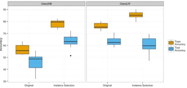
4.2.1 Overfitting 61

4.3 Outliers, overlapping classes, and minority classes 64

4.3.1 Outliers 64

4.3.2 Overlapping classes 68

(5)

4.3.4 Summary 72

4.4 Comparative results 73

CHAPTER 5. CASE STUDIES 76

5.1 Parameter tuning 76

5.2 Case studies 77

5.2.1 Nodal metastasis in major salivary gland cancer 79

5.2.2 Mortality after Nephroureterectomy for Upper-tract Urothelial Carcinoma 85

5.3 Rules of thumb for instance selection parameters 91

CHAPTER 6. CONCLUSIONS 97

6.1 Future work 98

APPENDIX. TABLED RESULTS 100

(6)

ABSTRACT

Aspects of a classifier’s training dataset can often make building a helpful and high accuracy classifier difficult. Instance selection addresses some of the issues in a dataset by selecting a subset of the data in such a way that learning from the reduced dataset leads to a better classifier. This work introduces an integer programming formulation of instance selection that relies on column generation techniques to obtain a good solution to the

problem. Experimental results show that instance selection improves the usefulness of some classifiers by optimizing the training data so that that the training dataset has easier to learn boundaries between class values. Also included in this paper are two case studies from the Surveillance, Epidemiology, and End Results (SEER) database that further confirm the benefit of instance selection. Overall, results indicate that performing instance selection for a classifier is a competitive classification approach. However, it should be noted that instance selection might overfit classifiers that have already achieved a good fit to the dataset.

(7)

CHAPTER 1. INTRODUCTION

This chapter will introduce the concept of instance selection for classifier training along with its benefit and the objectives of this dissertation. At the end, an overview of the dissertation’s contents is presented.

1.1 Motivation

The world is inundated with information and it is advantageous to extract as much knowledge from that information as possible. Some practices that help accomplish this task are grouped into the area of data mining, and one particularly helpful practice is known as classification.

In data mining, information is arranged into a collection of data points called

instances. Each instance can describe a particular object or situation and is defined by a set of independent variables called attributes. For classification problems there is a target concept we wish to learn about and this concept is represented in each instance as a

dependent variable having finitely many values called the class. The goal of classification is therefore to construct a model from instances with known class values, called the training dataset, to predict which class an instance should belong to based on its observed attribute values. In some cases the induced classification model, or classifier, is simply used to make class predictions for instances with unknown class values, while in other cases the classifier is analyzed to learn more about the target concept. The quality of the learned model is typically assessed by calculating the number of correct predictions made by the classifier when predicting the class values of a withheld set of instances called the testing dataset.

(8)

The goal of this research is to provide a method to create better classification models, or as that often implies, classification models with higher testing accuracy. Better

classification models will be obtained by optimizing the training data in such a way that the training dataset has easier to learn boundaries between class values. The motivation for this is that numerous aspects of the training data can make it difficult for a classification learner to induce an accurate model. For example, two class values may completely overlap, one or more classes may have outliers, or minority class values may exist that can be ignored by the learner. A relatively recent approach for addressing such issues is to use what has been termed instance selection to create a subset of the training dataset in such a way that all or some classification learning algorithms will perform better when applied to the new and reduced training dataset.

Clearly, instance selection may be thought of as a combinatorial optimization problem where each instance is either included or not, that is, a problem with a binary decision variable, resulting in a search space of 2 possible subsets of instances. As may be very large, searching through this space without structure is very difficult. Furthermore, the ultimate objective function is to maximize the test accuracy of the classifier induced on the selected instances; that is, the objective function has no closed form and can only be evaluated on an independent test dataset after a classification model has been learned. One can use a proxy of the test accuracy, e.g. the accuracy on the training data, but even then the objective function has no closed form and is difficult to evaluate. Perhaps due to those reasons past work on instance selection has focused heavily on the use of metaheuristics, primarily evolutionary algorithm, that search the space of 2 possible instance subsets directly without attempting to place any structure on the search space or utilize any

(9)

optimization theory. Thus, while numerous connections between optimization and

classification have been thoroughly studied in the literature (Olafsson et al., 2008; Bradley et al., 1999), it is contended that the understanding of instance selection as an optimization problem is still in its infancy.

1.2 Research

objectives

The premise of this dissertation is that the boundaries between instances with different class values in the training data can be optimized for the induction of a classifier through an integer programming (IP) formulation of instance selection. This draws on optimization theory to create a search space (formulation) that can be searched to find a better set of the training data; that is, training data with boundaries more suited to the chosen classifier, which subsequently leads to a better (high- accuracy) classification model. The overall objective of this dissertation is thus to develop optimization theory and methods for instance selection, focusing primarily on an integer programming formulation of instance selection.

A naïve integer programming formulation of instance selection is very straightforward. The decision variable could be defined as,

1 if instance is included in the final training data 0 otherwise.

The objective function could then be to maximize the accuracy of some model (e.g., a decision tree) learned on the selected instances, and no further constraints are required. However, this objective function has no closed form and the feasible region has no structure that can be exploited to help search through this space of 2 possible solutions (where is the number of instances).

The contention of this dissertation is that instead of naively solving this problem using some heuristic, the formulation should be rethought to make it more solvable. One of

(10)

the key novel ideas of this dissertation is thus to construct subsets of instances that appear to perform well together, that is, instances that when considered together lead to a classifier with high accuracy. A column can then be defined as … where 1 if instance is included in the th column (subset), and 0 otherwise. The decision variable of the integer programming problem is then to decide which columns’ instances should be used in the final training data, that is,

1 if column instances are included in the final training data

0 otherwise.

Additional constraints may now be relevant. For example, let denote the set of all columns, and formulate the instance selection problem as

1

. 1, ∀

2 0,1 , ∀ . 3

The objective is still to maximize classifier accuracy and the constraint ∑ _∈ 1 ensures that each instance is selected for the final training data at most once. One may recognize this constraint as a set packing constraint, as the set packing problem is a well-studied IP problem. However, for reasons outlined below, the pure set packing formulation may not be the best formulation of the instance selection problem.

The key to a good formulation of the instance selection problem is the ability to generate good columns, that is, to construct subsets of instances that work well together. This leads to the first explicit research question addressed in this dissertation.

(11)

Research Question 1: When formulating a set-packing-type IP for instance selection, how should a good initial set of columns be constructed?

Regardless of the specifics of the instance selection formulation, a key issue is to determine a set of columns (subsets) to be used in the IP. Motivated by similar approaches that have been found effective for both set covering and partitioning problems, the process is initiated by generating good initial columns ’, which can then be improved (see Research Question 2 below).

Research Question 2: Given a set of initial columns and an IP formulation of instance selection, how can column generation be implemented to find improving columns?

In traditional column generation a linear program (LP) with a prohibitively large number of decision variables (or columns) is solved to optimality without having to consider or construct all of its possible columns. This is accomplished by considering a relaxation of the original LP that contains only a subset of the possible columns and generating any new columns needed to improve the relaxation’s solution. Through an iterative process

eventually no improving columns can be generated and it is known that the optimal solution to the original LP is found.

Column generation is an ideal technique to construct good columns for instance selection because of the prohibitively large number of possible columns. Even though column generation is designed specifically for solving LPs it is frequently used in integer programs by relaxing the integrality constraint of the decision variables, and this is no different when considering instance selection. However, unlike traditional column

(12)

because there is no closed form function to calculate the accuracy of a classifier based solely on the contents of its training data.

Therefore, to effectively implement column generation with the purpose of finding improving columns for an IP formulation of instance selection, an estimation of classifier accuracy based on the content’s of its training data is required.

Research Question 3: When formulating instance selection using IP, what constraints should be placed on the selection of columns in addition to the set packing constraints?

The formulation of instance selection in equations (1) through (3) is only one of the many instance selection IPs that could be devised, and it is not without its own shortcomings. For example, adding a constraint ∑ _∈ 1 to (2) and (3) insures that a simple linear

objective function can be defined for the instance selection integer program. While this is a plausible approach and preliminary results indicate that column generation is able to discover useful columns based on a relaxation of this IP, it also somewhat restricted. In fact, it is known that allowing more than one column can be advantageous as preliminary results also show that a greedy search can be used to select amongst the columns to combine them in a useful way. Two IP formulations of instance selection with different goals in regard to column generation are discussed in Chapter 3.

1.3 Organization of dissertation

Chapter 2 of this dissertation presents a review of the relevant literature related to data mining, instance selection, and column generation. Chapter 3 follows with two formulations of instance selection as an integer program, as well as considerations for

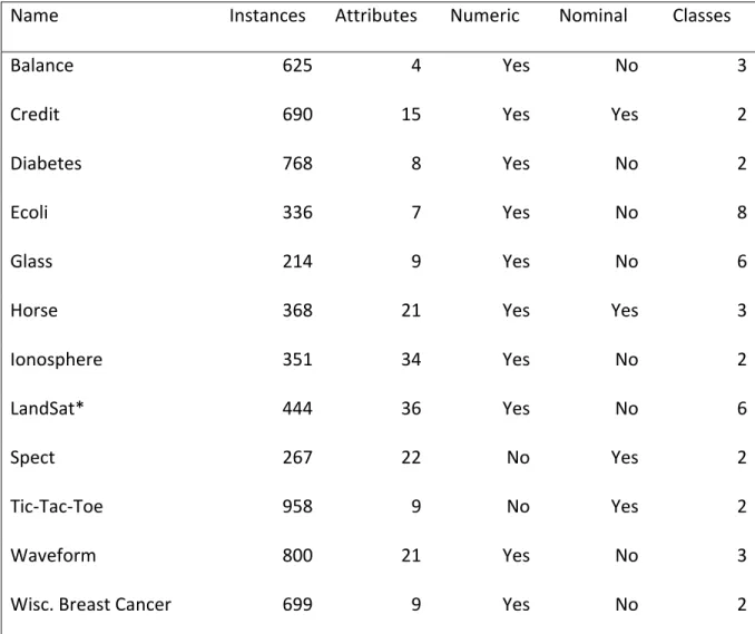
column generation. Chapter 4 introduces results from 12 experimental datasets along with an analysis of instance selection. In Chapter 5, two case studies concerning the Surveillance,

(13)

Epidemiology, and End Results (SEER) database and instance selection are discussed. Finally, conclusions and suggestions for future work are made in Chapter 6.

(14)

CHAPTER 2. LITERATURE REVIEW

Chapter 2 will introduce data mining, instance selection, and column generation. This will provide the reader with sufficient background information to follow the concepts of the dissertation and to show the current gap in the instance selection literature.

2.1 Data

mining

Data mining has been found to be increasingly useful in many application areas (Han and Kamber, 2003; Witten and Frank, 2005). This can partially be contributed to increased prevalence of massive databases, which often contain a wealth of data that traditional methods of analysis fail to transform into relevant knowledge. Specifically, meaningful patterns are often hidden and unexpected, which implies that they may not be uncovered by hypothesis-driven methods. In such cases, inductive data mining methods, which learn directly from the data without an a priori hypothesis, can be used to uncover hidden patterns that can then be transformed into actionable knowledge.

All data mining starts with a set of data called the training set, which consists of instances describing the observed values of certain variables, or attributes. These instances are then used to learn a given target concept or pattern. One such approach is classification. In classification the training data is labeled, meaning that each instance is identified as

belonging to one of two or more classes, and an inductive learning algorithm is used to create a model that discriminates between those class values. The model can then be used to classify any new instances according to this class variable. The primary objective is usually for the classification to be as accurate as possible.

(15)

Five useful and common classification algorithms are k-Nearest Neighbors (k-NN), naïve Bayes, decision tree, logistic regression, and support vector machines. Each of these classification algorithms, with the exception of k-NN, operates by inducing some model from the training data that can then be used to predict the class of unlabeled instances. However, each of these classifiers has an intrinsic bias that stems from assumptions made by the algorithm during its construction. This bias will cause the classifier to perform better for classification problems whose instances exhibit certain relationships amongst their attributes and true class labels. Although no classification problem may perfectly fit the assumptions made by any specific classification algorithm, it has been found that classifiers are still able to take advantage of some of the relationships and structure in the data and make good classifications. The five classifiers mentioned above will now be discussed along with their inherit biases.

K-Nearest Neighbors is an instance-based classifier. Meaning, the classification of an unlabeled instance is not based on any abstraction of the training data, but rather, is based on the training instances themselves. With k-NN an unlabeled instance is classified as the most prevalent class observed in the nearest k training instances. A positive of the k-NN classifier is that it is very simplistic, but this simplicity comes at the sacrifice of having to store large amounts of data and perform a large number of calculations every time that an instance needs to be classified. The bias of k-NN comes from the assumption that an unlabeled instance should be classified the same as its nearest neighbors. This assumption means k-NN will perform better for classification problems where instances belonging to different classes do not overlap and are separated by a large distance in Euclidian space.

(16)

Naïve Bayes is a statistical classifier that predicts the probability that a given instance belongs to a particular class. It is an attractive classifier because it requires only simple calculations and has been shown to have good accuracy for a wide variety of classification problems. The probability prediction of naïve Bayes operates under the assumption that the “effect of an attribute value on a given class is independent of the values of the other

attributes” (Han and Kamber, 2003). This assumption allows the required calculations of the classifier to be simple, but also introduces a bias to the classifier. Specifically, the naïve Bayes classifier is biased in a way that it performs better when an instance’s attribute values affect its class outcome with higher levels of independence.

Decision trees are another popular and relatively simple technique for classification. Decision tree algorithms induce a tree in a top-down manner by selecting attributes one at a time and splitting the training instances into groups according to the values of their attributes. The most important attribute is selected as the top split node, the next most important

attribute is considered at the next level, and so forth. For example, in the popular C4.5

algorithm (Quinlan, 1992), attributes are chosen to maximize the information gain ratio in the split. This is an entropy measure designed to increase the average class purity of the resulting subsets of instances as a result of the sequential splits. A bias intrinsic to decision trees is of course that they perform better when an instance’s attributes actually have a hierarchical structure in regard to determining class label.

Logistic regression is a classification technique closely related to linear regression. However, unlike linear regression the outcome is not a predicted numerical value, but instead is a probability prediction that an instance belongs to a specific class. This prediction is achieved by creating a linear function of the dataset’s attributes. Again, as with the other

(17)

techniques that create a classification scheme from the data, a bias is introduced. This time the bias is that logistic regression works better when an instance’s class is actually

determined by some linear function of its attribute values.

A support vector machine is a classification technique that identifies instances (or support vectors) that help define the optimal border between classes. Support vectors are typically found by transforming the original data with some non-linear mapping to a high dimension space and then implementing an optimization problem to find an optimal hyper plane that separates the instances into different classes. Support vector machines have been found to be very useful in practice as they can achieve high accuracy while avoiding

overfitting. Still, support vector machines have a bias and the challenge is to find an appropriate kernel that maps the instances to a space in which they are truly separable.

Because classification algorithms have biases and because natural classification problems do not perfectly fit this bias, classifiers are quite frequently less than perfect. To combat these imperfections many researches have suggested improvement techniques. In fact, instance selection is one such class of techniques and will be discussed in great detail later. Another class of improvement techniques is ensemble classifiers. Ensemble classifiers make a prediction for an unlabeled instance by consulting multiple classifiers and using a voting scheme to make a final determination. The idea behind ensemble classifiers is that a deficiency in one classifier may be compensated for in the other classifiers, and that the majority decision has greater potential to be correct. Two ensemble classification techniques are AdaBoost and random forests.

AdaBoost is an ensemble classifier that builds sequential classifiers from a training dataset. At the beginning, a classifier is built from the training dataset with all of the

(18)

instances having an equal weight. This classifier is then used to classify the original training data. Any instances that are misclassified by the classifier have their weight increased so that the classifier built next will give them more attention. This process of building a classifier and adjusting instance weights continues until a sufficient number of classifiers are

constructed. An unlabeled instance can then be classified through a voting scheme where each constructed classifier gets a weighted vote. The weight of each vote corresponds to the accuracy of the classifier that cast it. AdaBoost is an effective technique to increase the accuracy of simple classifiers, but interpreting the constructed classifier is difficult because a prediction is not the result of a single classifier.

Random forest is an ensemble technique that utilizes decision trees. Similar to AdaBoost it operates by creating a large number of decision trees and uses a voting

mechanism to assign a class to unlabeled instances. A single decision tree in random forest is created using a random subset of the training data’s attributes. Additionally, the training data for a single decision tree has randomness introduced through bagging, which is sampling the original training data with replacement (Brieman, 2001). It has been found that random forest can achieve quite good accuracy in comparison to other methods, but again

interpreting the constructed classifier is difficult.

2.2 Instance

selection

The process of instance selection was first utilized for instance based classifiers, such as k-Nearest Neighbors (k-NN), because faster and less costly classifications could be

obtained by maintaining only certain necessary instances in the classifier’s dataset (Hart, 1968; Ritter et al., 1975; Wilson, 1972). That is, because instance based classifiers perform calculations for each instance of a dataset every time a new classification is to be made, a

(19)

smaller dataset would require a smaller amount of memory storage and a fewer number of calculations. The goals of the first instance selection algorithms were therefore to select the minimum number of instances required to maintain the current classification accuracy of a dataset (Hart, 1968). However, it has been found that instance selection not only reduces the size of the dataset, but it also improves the dataset quality by not selecting to maintain outlying, noisy, contradictory or simply unhelpful instances (Sebban et al., 2000; Zhu and Wu, 2006; Olvera-Lopez et al., 2010).

As a consequence of instance selection’s ability to improve the quality of a dataset, a developing use of instance selection outside of instance based classifiers is to select good training datasets for learning a classification model, such as with the decision tree or neural network classifiers. This area of instance selection is different than early methods used for instance based classifiers because the goal is no longer data reduction but it is rather to maximize classifier accuracy. However, a good selection of instances for an instance based classifier may not lead to the best training dataset for another type of classifier, indicating methods that incorporate the intended classifier in the learning process are warranted

(Olvera-Lopez et al., 2009). In fact, it is this author’s belief that using the intended classifier in instance selection procedures is beneficial because instances that obscure advantageous structure or relationships in regard to the classifier’s bias can be removed. This makes learning good boundaries between class values easier for the classifier. Therefore, with the majority of instance selection algorithms being developed for instance based classifiers, effort should be given to develop instance selection algorithms that are applicable to other classification methods used in practice.

(20)

A recent review paper notes that the majority of instance selection methods for training set selection find an acceptable set of training instances utilizing random search with evolutionary algorithms (Garcia-Pedrajas, 2011). Evolutionary algorithms are a popular search technique because they are capable of taking into consideration the particular bias of a specific classification algorithm, and as such, lead to a good selection of training instances for that classifier. Most instance selection methods for training set selection are designed for neural networks and decision trees, but could be adapted for a variety of different

classification algorithms that learn a classification scheme from a training dataset. The majority of the evolutionary algorithms attempt to maximize training accuracy as a proxy for testing accuracy, where training accuracy is the percentage of correct predictions made by the classifier when predicting the original training instances, and where testing accuracy is the percentage of correct predictions made when predicting instances withheld from the training process (Han and Kamber ,2006).

Training set instance selection procedures for neural networks serve to increase the generalization ability of the networks by selecting good instances on which to train. These procedures should be beneficial to neural networks because in the presence of noisy data, the networks become overfitted to the training dataset and subsequently are poor classifiers to unseen instances (Kim, 2006). Reeves and Taylor (1998) and Reeves and Bush (2001) perform instance selection for radial basis function (RBF) nets with evolutionary algorithms where the fitness of a solution is determined by the training accuracy of the RBF net, and the instances contained in the training dataset are evolved. It is found that indeed the

generalization performance of RBF nets can be increased through training set instance selection. Kim (2006) also performs instance selection for increased generalization ability,

(21)

but this work is focused on feed forward neural networks and financial forecasts. Here, an evolutionary algorithm determines the training instances and the structure of the network, and the fitness of a solution is evaluated by the training accuracy of the network. Again, the results indicate that the generalization performance of neural networks can be improved by selecting instances to create a higher quality training dataset.

The decision tree classifier is another popular choice for training set instance

selection because unhelpful instances in the decision tree’s training dataset cause the tree to unnecessarily grow its structure (Sebban et al., 2000; Oates and Jensen, 1997). This

overfitting problem defeats the purpose of the decision tree by hiding or confusing the discovered knowledge in a large and un-interpretable tree structure that has poor

generalization abilities. Performing instance selection often results in a smaller and more interpretable tree, an indication that the unhelpful instances have not been selected. Endou and Zhao (2002), Cano et al. (2003), and Cano et al. (2006), evolve the instances contained in a subset of the training dataset in the hopes of finding a collection of instances that adequately describe the full dataset. Endou and Zhao (2002), as well as Cano et al. (2006), evaluate the fitness of the selected training dataset through the construction and evaluation of a decision tree from the training dataset, and both of these methods are successful in reducing decision tree size, while still maintaining acceptable, if not improved, levels of accuracy. Cano et al. (2003) evaluates the fitness of the training dataset using the 1-NN classifier, and interestingly, this method is also successful in creating simple, yet accurate, decision trees. These methods indicate that decision tree learning can indeed be improved by selecting a good set of training instances through instance selection.

(22)

One exception to the usual pattern of training set instance selection is found in a paper by Zhu and Wu (2006), where the training dataset’s instances are put into groups of similar instances, and then some of the groups are greedily selected to form a reduced training dataset with the goal of improving the classification training accuracy of the naïve Bayes and decision tree classifier. This work is notably different from other methods because instead of performing an evolutionary algorithm to select a training dataset from individual instances, a greedy selection procedure is used to select a training dataset from the created groups. Results show that this method is also successful in increasing classification accuracy.

Another notable exception to the usual pattern of training set instance selection is work done by Olvera-Lopez et al. (2009). In this paper a greedy selection procedure is developed that incrementally subtracts instances from the training data to achieve a suitable subset of instances for classifier learning. This is not unlike Bennette and Olafsson (2011), with the exception that Bennette and Olafsson extend the idea by creating a large number of such subsets with the intent of recombining them in a way that results in even better

classification accuracy.

In all cases, previous instance selection techniques do not attempt to create a solvable formulation of the instance selection problem. Instead, most techniques are content to employ heuristics that simply search a prohibitively large solution space. This dissertation breaks the trend and presents an integer programming formulation of instance selection that has structure which can be exploited to find improving selections of instances.

2.3 Column generation for LPs

Column generation is a set of techniques to solve linear programs (LP) that have a huge number of variables (Desrosiers and Lubbecke, 2005; Wilhelm, 2001). In column

(23)

generation the original LP is called the master problem (MP). Column generation is useful when it is too computationally expensive to solve the MP with all of the original variables or when it would be too computationally expensive to even enumerate all of the decision variables. There are several approaches to column generation, but each involves solving a reduced portion of the MP, called the reduced master problem (RMP). One approach to column generation, commonly referred to as Type I column generation, uses an auxiliary model (AM) to find a subset of the MP’s useful variables and then supplies those to the RMP with the hope that the RMP will find a good feasible solution to the MP. However, because not all variables are considered, the solution to the RMP cannot be guaranteed to be optimal to the MP. Another approach to column generation, Type II column generation, also

involves supplying the RMP with a subset of the MP’s variables. However, in this approach, the RMP is solved and then its dual variables are supplied to a price out problem (POP). The POP generates another decision variable of the MP that will allow the RMP to improve its solution. The RMP is then resolved with the new and improved decision variable, creating a new set of dual variables. The POP can continue to interact with the RMP and generate improving variables until the optimal solution of the MP is found.

2.3.1 Type I column generation

Say there is a linear program (LP) max : , 0 , which is so large that defining all of its possible variables is computationally impractical. Defining a variable

requires defining and , where is the objective coefficient associated with variable and is the column of the matrix defined by variable . The LP with all of its variables defined will be called the master problem (MP). However, only a small number of the possible variables can actually be known or be provided to the RMP. Therefore the reduced

(24)

master problem (RMP) can be defined as max ∶ , 0 , where contains only the known variables and and contain the objective and constraint values for those variables.

In Type I column generation the RMP is provided high quality decision variables from the auxiliary model and then solved. Even though the optimal solution to the RMP is a feasible solution to the MP, it cannot be guaranteed to be the optimal solution to the MP. Therefore, it is hoped that the optimal solution to the RMP is an acceptably good feasible solution to the MP, mainly because the solution is found from what are considered good decision variables (Wilhelm, 2001). Alternatively, Type II column generation provides a method to guarantee that the optimal solution to the MP is found.

2.3.3 Type II column generation

Type II column generation exploits a feature of the Simplex algorithm for solving linear programs. Say there is a known feasible solution to max : , 0 . For a standard form LP any feasible solution can be written in terms of the basic and non-basic variables. The Simplex algorithm moves to the optimal solution of the LP by switching variables from the basis to the non-basis in a way that improves the current feasible solution. The reduced cost is calculated for each variable belonging to the non-basis during an iteration of the Simplex algorithm, and when there are no non-basis variables with positive reduced cost, the optimal solution to the LP has been found. Type II column generation provides a method to avoid examining every variable during the Simplex algorithm and for linear programs that are so large they are infeasible to solve, this procedure can make them solvable.

(25)

As in Type I column generation, say there is a very large LP. The LP with all of its decision variables defined is the master problem (MP), and the restricted master problem (RMP) max ∶ , 0 is the LP with only the known decision variables defined. Now the optimal dual variables can be used in the price out problem (POP) to check if the optimal solution to the RMP is optimal to the MP. Failing to find that the solution is truly optimal, the POP can provide a new variable for the RMP. This new variable will have positive reduced cost, and by definition can improve the RMP’s solution. The RMP can then be resolved, provide new dual variables to the POP, and the process repeated until no new positive reduced cost variables can be generated.

The formulation of a POP is specific to every RMP, but contains the same basic objective function and should be capable of generating all of the undefined variables

belonging to the master problem. The objective of a POP is to maximize the reduced cost of a newly generated variable . The objective of every POP should therefore be

max ∗ _{, where} _{is the objective coefficient of} _, ∗_{are the optimal} dual variables to the RMP, and anew_is_{the column of the matrix to be associated with} _. Provided constraints in the POP are able to dictate how the new variable affects constraints in the RMP, and given a method to calculate the objective coefficient of the new variable, Type II column generation is complete. When solving the POP if the optimal objective value is less than or equal to zero, indicating there are no positive reduced cost variables, it is known that the solution to the RMP is optimal to the MP. Otherwise the new variable should be added to the RMP and the process repeated.

(26)

CHAPTER 3. MODEL FORMULATION

This chapter includes two separate integer programming formulations of instance selection. Each formulation is designed to facilitate column generation procedures that can help find improving subsets of instances (or columns). Also discussed in this chapter are procedures to create initial sets of columns, the development of column generation for instance selection, necessary approximations for the price out problems, and a discussion of instance selection parameters.

3.1 Integer programming formulations of instance selection

The primary research objective of this dissertation is to find a structured integer programming formulation of instance selection. The motivation for doing so is to impose a structure on instance selection that will help guide a search for improved subsets of the training data. The two formulations are as follows,

∈ 4 . 1, ∀ 5 0,1 , ∀ 6 , and, ∈ 7

(27)

. 1

8

0,1 , ∀ 9 .

In both formulations the decision variable represents the decision to include or not include a subset of the instances (column), S(j)_{, in the final training dataset. Associated with} each column S(j)_{, is a vector} _._If _{, an element of , has value one it indicates that the}_ith instance of the training datasetis included in column S(j)_,_{otherwise it is not}_._{This means that} if the column is included in the final training dataset, or 1, and the instance is in that column, or 1, then the ith_{instance is included in the final dataset. The objective of} each formulation is simply to maximize the accuracies of the selected columns, where is the accuracy of the jth_{column, or as that implies the accuracy of a classifier built from the} instances in column S(j)_.

Unfortunately for large datasets it is computationally impractical to enumerate all of the 2 decision variables that define J, where is the number of instances in the training dataset (indexed by I). To resolve this issue, concepts from column generation are used to generate what are felt to be good decision variables for the instance selection problem. That is, column generation is used to generate columns that have good accuracy. After a number of good columns are generated, any number of solution procedures can then be used to obtain a suboptimal, but hopefully good, solution. A Type II column generation procedure for each of the above IP formulations encourages the generation of different but helpful types of columns.

(28)

The logic behind the first integer program, (4) through (6), is that the instances of the IP’s most accurate columns should be included in the final selection of instances. This formulation acknowledges the fact that the most accurate column of a dataset is unlikely to be found, and that combining the instances of good columns may be helpful. However the constraint defined by (5) says that selected columns should be disjoint, meaning they should not have any instances in common. The result of this formulation should be a column

generation procedure that strives for ever-improving and diverse columns. Meaning, column generation should generate new columns that are similar to existing columns, but that result in higher accuracy.

The second IP formulation, (7) through (9), has a constraint that says only one column can be selected by the IP, ∑ _∈ 1. It should be noted that this constraint also enforces the constraint defined in (5). The logic behind such a constraint is that the final training dataset should include only the instances of the most accurate column, and including any additional columns will not be helpful. This formulation would perfectly solve the instance selection problem, except, as mentioned earlier, finding the most accurate column for a dataset is unlikely. Still, this IP is attractive in a column generation procedure because any newly generated column must have accuracy higher than that of the previous best column. This may lead to the discovery of very useful columns.

Before Type II column generation can be implemented an initial set of columns needs to be generated. This can be accomplished with what can be thought of as a Type I column generation procedure. Each IP can utilize the same initial set of columns and three such methods are introduced in Section 3.2.

(29)

3.2 Constructing initial sets of columns

It is believed, and observed in preliminary experiments, that a set of initial columns for the provided IPs should be diverse and contain helpful instances. By diverse it is meant that the combination of instances included in a particular column is unique to that column, and dissimilar to combinations found in other columns. Additionally, a column is thought to include helpful instances if the accuracy of a classifier built from those instances has high accuracy. Three approaches to create initial sets of columns are introduced, each imposing varying levels of instance diversity and helpfulness.

Each approach to creating initial columns for the instance selection IPs relies on an auxiliary model akin to that needed for Type I column generation. The first two methods use greedy selection procedures that incorporate the base classifier of the instance selection problem, meaning the classifier considered for improvement, and the last method simply constructs initial columns with randomly included instances. Each method results in the creation of a column for every instance. This means that every instance is guaranteed to be included in at least one column, and the number of columns created is the same as the number of instances in the training data.

3.2.1 Backward selection

In the case of the backward selection procedure, a single column, S(j)_{, initially} contains all of the original training instances, and instances are removed from the column if doing so does not greatly hinder the predictive accuracy of a classifier built from that column. In this way it is thought that columns will contain helpful instances, because instances necessary to preserving classifier accuracy remain in the constructed columns. To introduce diversity to the constructed columns instances are considered for removal from the

(30)

columns in a random order. Additionally, to ensure that each instance is represented in at least one column, each instance generates a column where that instance is not considered for removal. Pseudo code for the Backward Selection Algorithm is provided below. Note that “Predictive Accuracy” can be calculated by constructing the base classifier from the provided instances and evaluating it on the original training data.

Backward Selection Algorithm Step 0: , , … , | | , . Step 1: 1 , , … , , , … , 1 , . Step 2: 1 1 1 / / .

(31)

3.2.2 Forward then backward selection

In the case of forward then backward selection, columns begin empty except for a single instance, and instances that improve the accuracy of the column are added in a greedy fashion. Once all of the original training instances have been considered for addition to the column, all of the accepted instances are then considered for removal in a greedy fashion. Instances are only removed from the column if doing so does not greatly hinder the column’s accuracy. As with the strictly backward selection method, a column is constructed for each instance of the original training data and instances are considered for addition to the column and subtraction from the column in a random order.

This method strives to find columns that contain only helpful instances by allowing all instances that improve the accuracy of the column to be included in the column.

However, in preliminary experiments it was found that a strictly forward selection procedure seemed to include instances that were only marginally helpful. It was then found helpful to consider removing instances from the columns. This is presumably the case because some instances added later in the forward selection procedure could serve the purpose of some of the instances added early on. Below is pseudo code for the Forward then Backward

Selection Algorithm, where “Predictive Accuracy” is calculated as before. Forward then Backward Selection Algorithm

Step 0:

, , … , | |

, .

Step 1:

(32)

, , … , 1 , . , , … , 1 , . Step 2: 1 1 1 ∪ ∪ Step 3: 1 1 1 / / .

(33)

3.2.3 Random selection

In the random selection procedure no classifier information is used to determine which instances are included in a column. Meaning, this method relies on random chance for helpful instances to be included in any one column. However, by definition, this method creates diverse columns. As with the previous methods a column is generated for each instance, where that instance is guaranteed to be included in the column. The remaining training instances are of course randomly assigned to the column. One additional

requirement of this method is for the user to decide how many instances should be included in a single column. This may require some background knowledge of the classification problem and classifier to make an informed decision. Pseudo code for the Random Selection Algorithm is shown below.

Random Selection Algorithm Step 0: , , … , | | , . Step 1: 1 , , … , 1 , . Step 2: 1

(34)

1 1

∪ .

3.3 Implementing column generation

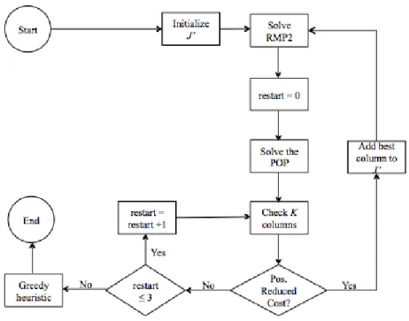
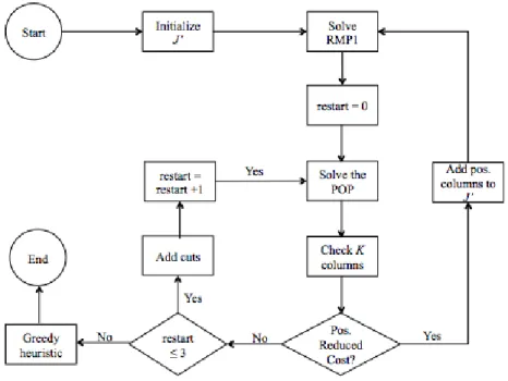
Given the two integer programming formulations of instance selection and three methods to create initial columns, a simple variant of Type II column generation can now be defined. To implement Type II column generation each integer program needs to have a master problem (MP) defined, a reduced master problem (RMP) defined, and a price out problem (POP) defined. Each MP is a linear relaxation of the original integer program, and the RMP is defined as the MP having only considered a subset of the possible columns. The POPs for each integer program are similar but have slightly different objective functions to generate valid columns for their respective IPs.

3.3.1 Implementation one

Consider the formulation of instance selection defined by the IP in (4) through (6). In order to implement a Type II column generation procedure the integrality constraints of (6) need to be relaxed. In this particular case it is reasonable to relax the integrality constraints because the resultant linear program restricts the number of times an instance can be selected for the final training data. Logically, the effect of this constraint combined with the objective function is that the MP will strive to select whole columns with high accuracy. In the actual column generation procedure the intended result will be variations of existing columns that have improved accuracy. The resulting MP is,

∈

(35)

. 1, ∀

11

0, ∀ 12

1, ∀ , 13 and the related RMP is,

∈ 14 . 1, ∀ 15 0, ∀ ′ 16 1, ∀ ′. 17

The POP is then,

. ∗ 18

. 19

(36)

0,1 , ∀ , 20 where we let Χ denote the feasible region defined by (19) and (20).

In this POP the decision variables are binary. When a specific ai assumes the value one, it represents the decision to include instance i in the new column, and ai equal to zero

represents the decision to exclude instance i from the new column. The sole constraint

∑_∈ restricts the number of instances selected to belong to a new column to be less than or equal to some constant G. This constant G allows the POP to directly control the size of the newly generated training data subsets. The objective of this POP is to maximize

reduced cost, but as stated previously, a closed form function is not known for calculating the accuracy of a classifier based on the instances it is trained from. This makes the POP

unsolvable, but in Section 3.4, approximation techniques to solve the POP will be presented.

3.3.2 Implementation two

Consider the formulation of instance selection defined by the IP in (7) through (9). In order to implement a Type II column generation procedure the integrality constraints of (9) need to be relaxed. However, the integrality constraints of (9) can be relaxed and still allow for an integer solution to be found, as will now be proven.

Lemma 1. Given that ∗ is optimal to max ∑ ∈ : ∑ ∈ 1, 0 1 ∀ ∈ , ∑ _∈ ∗ 1 when 0 ∀ ∈ .

Proof: Assume ∑ _∈ ∗ 1. Then there exists such that ∗ 1. Construct a new solution

′ such that ∗ 1 ∑ _∈ ∗ , and ∗ ∀ . Since 1 ∑ _∈ ∗ 1 ∗, then ∗ 1 ∗ and it follows that 1. Additionally, since ∑ _∈ ∗ ∑ ∗

(37)

∗_{, then}_∑

∈ ∑ ∈ ∗ 1 ∑ ∈ ∗ , and again it follows that ∑ ∈ 1. Finally, because ∑ _∈ ∑ _∈ ∗ 1 ∑ _∈ ∗ , and since 1 ∑ _∈ ∗ 0, it is true that ∑ _∈ ∑ _∈ ∗. There is a contradiction, ∗ is not the optimal solution. ∎ Lemma 2. If max then ∗ 0, where ∗ is the optimal solution to

max ∑ ∈ : ∑ ∈ 1, 0 1 ∀ ∈ , when 0 ∀ ∈ .

Proof: Assume there exists k such that max and ∗ 0. Given i such that

max define a new solution where ∗ ∗, 0, and ∗ ∀

. Since ∗ ∗ ∑ _∈ ∗ and ∑ _∈ ∗ 1, then 1. Additionally since

∑ _∈ ∑ ∗

∗ ∗ ∑ ∈ ∗, and ∑ ∈ ∗ 1, then ∑ ∈ 1. Next, because and ∗ 0, it is known that ∑ _∈ ∗ ∑ ∗ ∗. Finally, it can be shown that ∑ _∈ ∑ ∗ ∗. There is a contradiction, ∗ is not the optimal solution. ∎

Theorem 1. Given that 0 ∀ ∈ , max ∑ _∈ : ∑ 1, 0 1 ∀ ∈

has an optimal solution such that ∗ ∈ 0,1 ∀ ∈ .

Proof: Assume there is no optimal solution such that ∗ ∈ 0,1 ∀ ∈ . Because of Lemma 1 it is known that ∑ _∈ ∗ 1. Because of Lemma 2 it is known that for any : ∗ 0 then

max , say k. It can then be shown that ∑ _∈ ∗ ∑ _∈ ∗ . Define a new

solution . Choose some such that k. Then define 1, and 0 ∀ . Then

∑ _∈ ∑ . It is then known that ∑ _∈ ∑ _∈ ∗. The new

(38)

The required relaxation of (7) through (9) is permissible because as Theorem 1 shows, there is always an integral optimal solution to the relaxed IP. This relaxation makes intuitive sense because it would be suboptimal to select a portion of any column that did not have the highest available accuracy. If two or more columns are tied for the highest accuracy it would be possible to select non-integer portions of each of those, but an optimal integer solution is still possible by selecting the entirety of one column. The result of this fact is that columns generated in the Type II column generation procedure will have higher accuracy than any of the existing columns. The resulting MP is,

∈ 21 . 1 ∈ 22 0, ∀ 23 1, ∀ , 24 and the associated RMP is,

∈ 25 . 1 ∈ 26 0, ∀ ′ 27

(39)

1, ∀ ′. 28 The POP is then,

. ∗ ∗ ₂₉

. 30

0,1 , ∀ , 31 where we let denote the feasible region defined by (30) and (31).

The POP formulation is identical to (18) through (20) except that the objective function automatically subtracts the last dual variable. This change simply enforces constraint (26) in the RMP. As before, this POP is not solvable because no closed form function is known to evaluate the accuracy of a classifier based on the contents of its training data. Section 3.4 presents approximation methods for solving the POP.

3.4 Approximating the price out problem

The price out problems defined in (18) through (20) and (29) through (31) are not solvable because there is no known closed form function for calculating the accuracy of a classifier based solely on the contents of its training data. However, if some approximation of classifier accuracy is substituted for actual accuracy, approximations of the price out problems can be solved. The objectives become to generate a column that maximizes an estimation of reduced cost. Any generated column can then be checked for truly positive

(40)

reduced cost by simply building the associated classifier and using its accuracy in the reduced cost calculation. If the column is indeed beneficial to the RMP it can be added, if it is not, a new column can be generated and considered.

Generating improving columns with an estimated POP requires a good method to predict the usefulness of a classifier based on its training data. Two methods that have been successful in preliminary tests are presented in this section. Both methods find a ranking of the instances and operate under the assumption that the more high-ranking instances

contained in a training dataset the higher the accuracy of the resultant classifier. Note that the sum of the ranks of the instances included in a classifier’s training data does not represent a prediction of the classifier’s accuracy. Rather the sum represents an indication of the classifier’s potential usefulness.

Because ranking instances does not result in a prediction of classifier accuracy, but rather a prediction of usefulness, the rank and dual variables used in the estimated POPs are scaled between zero and one. This scaling ensures a fair comparison when considering whether or not to include an instance in a new column. For example, if an instance is ranked relatively high, but has an associated dual variable that is also relatively high, it may not be a good instance to include in the generated column. Of course, it is not ideal to require that the rank of instances and the optimal dual variables be scaled, but it is necessary until some linear approximation of classifier accuracy is developed.

The two methods used to rank instances are discussed in the following subsections. The first relies on information theory and some minor pieces of empirical evidence. The second relies solely on empirical evidence. The ranking procedures allow the POP defined in (18) through (20) to be replaced by,

(41)

∗ _{: ∈} _{, 32}

and the POP defined in (29) through (31) can be replaced by,

∗ ∗ _{: ∈} _{. 33}

In both (32) and (33) r represents a scaled ranking of the instances, achieved using the first or second method, and ∗ are the scaled optimal dual variables.

3.4.1 Ranking instance usefulness through information theory

The first method used to rank the usefulness of the training instances is adapted from Zhu and Wu (2006) and does so by quantifying the information lost as a result of a column of instances being removed from the training data. If a large amount of information is lost, or as that implies, a classifier suffers in accuracy and assuredness, it is assumed that the instances contained in the removed column are important to building a good classifier. The more important an instance is deemed to be, the higher its resulting rank.

To quantify the information lost through the removal of a column of instances from the training data, the log loss function is introduced. The log loss function is used to help quantify how much information is lost about a specific instance, say , by a classifier. This function, shown in equation (34), relies on the true distribution of an instance given by

| , and the predicted distribution of an instance given by | , where y is a class value of . The actual calculation is the negative sum over all possible class values of the true probability that an instance belongs to class y, times the log value of the predicted probability that the instance belongs to class y. The result of the calculation is that the

(42)

more incorrect a classifier is about the true distribution or class of an instance , the higher its value of . The lower bound of this calculation is zero, and there is no upper bound.

| |

34

To utilize the amount of information lost by a classifier about a specific instance, one final calculation is introduced. The behavior of a classifier for an instance , say , relays the quantification of information loss, but also incorporates whether or not a correct

classification is made for the instance. If a classifier makes the correct class prediction for , is equal to 0.1 to the power of . If the classifier makes the incorrect class prediction, is equal to -0.1 to the power of . This calculation is summarized in (35). The result of this calculation is that if a classifier loses little information about an instance, and it makes the correct prediction, then is high. If the classifier loses little information, but makes the wrong prediction, then is low. Intuitively, the instances that a classifier is

knowledgeable about have a high value of . ranges between one and negative one.

0.1

0.1 35

The idea behind the proposed ranking system is to see how the values of change after the removal of a column from a classifier’s training data. If the removed column has k

instances, then the average change in over all of the training instances is added to the rank calculation of the k instances. The logic is that if a column contains important instances, then the values of will decrease from their removal, and the average difference between the values will be positive. Given an initial set of columns, all columns can have the effect of their removal measured, and in the end, the instances with the highest rank are those

(43)

that belong to columns that hurt classification power when removed from the training data. The Information Rank Algorithm is summarized in the pseudo code below.

Information Rank Algorithm Step 0: , , … , , | |, , , … , , ⊆ , 0 ∀ ∈ . Step 1: ⋃ Step 2: 1 ′ ∩ ∈ 35 ′ 35 ′′ ∑ ∈ Step 3: 0 1.

(44)

3.4.2 Ranking instance usefulness through the frequency of instance occurrences The second method used to rank the usefulness of instances is based solely on empirical evidence. Specifically, this method ranks instances according to the frequency with which they appear in columns with high accuracy. Ranking instances this way is likely successful because the high accuracy columns hold instances which are known to work well for classification. If an instance appears frequently in these columns then it probably is indeed useful for classification, receives a high rank, and is prone to being included in new training data subsets. The specific implementation of the Frequency Rank Algorithm is shown in the pseudo code below.

Frequency Rank Algorithm Step 0: , , … , , | |, , , … , , ⊆ , 0 ∀ ∈ . Step 1: 1 ∈ 1 Step 3: 0 1.

(45)

3.5 Parameters

Instance selection as presented in this chapter requires a number of parameters to be set. These parameters are broken into two groups. First, parameters that require a choice, and second, parameters that require actual values to be chosen.

Choice Parameters:

 Which classifier to use

 Which reduced master problem (RMP) to use

 How to construct the initial columns (J’) of the RMP

 How to estimate reduced cost in the price out problem (POP)  How to measure accuracy

 How to combine columns for a final selection of instances

Value Parameters:

 The number of columns from which to estimate reduced cost in the POP, R

 The number of instances the generated columns in the POP can include, G

 The number of columns from the POP to check for positive reduced cost, K

 The number of restarts allowed in the POP

In the following subsections are descriptions of the different parameters that require tuning or a choice for the application of instance selection. Choice parameters will have the pros and cons of each choice analyzed. Discussed with the description of each value

parameter will be values that have worked in preliminary experiments, as well the potential benefit and harm of alternative values.

(46)

3.5.1 Which classifier to use

Instance selection should be performed with a specific classifier in mind. This classifier is used in the selection process and the goal is for the classifier to select instances that it can take more advantage of than the original training data. Preliminary results indicate that good classifiers for instance selection are naïve Bayes, logistic regression, and decision trees.

3.5.2 Which reduced master problem (RMP) to use

Both of the instance selection reduced master problems have promising properties for a column generation procedure, but they also both have shortcomings. The end goal of each RMP is to create high quality columns to be used in a search for the best selection of

instances from which to build a classifier. However, only one RMP will be considered when creating these improved columns for the instance selection procedure. A short description of each choice, RMP1 as shown in (14) through (17), and RMP2 as shown in (25) through (28), along with its positives and negatives is provided below.

Both RMPs are linear program relaxations of similar integer programs (IP). The IPs upon which each RMP is based, have the same decision variables and objective functions. The decision variables, called columns, can have value zero, indicating the column is not selected, and value one, indicating the column is selected. A column is a subset of the original training instances, and the accuracy of a column is the accuracy of a classifier built from the column’s instances as evaluated on the original training data. The shared objective function of each IP is to maximize the sum of the selected columns’ accuracies, and columns must be selected such that no instance appears in more than one selected column. With no additional constraints, the IPs select high accuracy yet disjoint columns.

(47)

RMP1, the first master problem, has no constraint limiting the number of columns that can be selected in the solution, and the optimal solution to RMP1 is not optimal to the IP upon which it is based. However, the objective function of RMP1 does encourage the

selection of disjoint high accuracy columns, making it useful. The price out problem of RMP1 leads to the generation of solutions that improve upon previous columns, where an improvement is considered a similar column that results in higher accuracy, but these improvements can pertain to any column currently existing in J’.

It is obvious that generating improved columns could be beneficial, as they may be attractive building blocks in the search for the best subset of instances. The downside of the formulation of RMP1 is that in the column generation procedure it is possible to create columns that are degradations of previously discovered columns. This seems to clutter the search space with unhelpful columns. It is possible to generate such columns because the objective function defining RMP1 can reward the addition of small, disjoint, and low accuracy columns. This will be impossible with RMP2.

RMP2, the second reduced master problem, has an additional constraint that no more than one column may be selected in the LP solution. The optimal solution to RMP1 is also optimal to the IP upon which it is based (see Theorem One). The solution of RMP2 is to select the highest accuracy column. This means with RMP2 that any improving column found in the column generation procedure must have higher accuracy than any column previously created.

The benefit from generating higher and higher accuracy columns is obvious. Very high accuracy columns could be a good starting point in the search for the best subset of instances. The downside of RMP2 is also its strength. Since the price out problem can only

(48)

generate columns with higher accuracy than the accuracy of columns previously discovered, potentially helpful columns in the search to find the best subset of instances may be omitted. For an example of such a column imagine a new column that has completely unique

instances from the current best column, but also has equal accuracy. This column is not discovered or considered in the price out problem of RMP2, but could obviously be

beneficial if considered in the construction of a high accuracy subset of training instances.

3.5.3 How to construct the initial columns (J’) of the RMP

J’ is the set of initial columns used to populate the RMP in the column generation procedure. It is known that the number of iterations required to solve a column generation procedure depends on this initial population. Even though column generation for instance selection will never be run to true optimality, it is clear that the quality of generated columns will depend on the initial columns of the RMP. One glaring reason for this dependency is that the two methods provided to estimate reduced cost depend on a subset of the columns from the RMP. For the early iterations of column generation the initial J’ is inextricably linked to the approximation of reduced cost.

Preliminary experimentation has shown that good initial columns of J’ should be diverse and contain beneficial instances (indicated by high column accuracy). However, it is not clear exactly how diverse the columns should be and how sensitive the procedure is to the inclusion of columns with non-beneficial instances. Five ways to create initial columns are summarized below, along with the positives and negatives of each.

The Backward Selection algorithm with equal to zero (B0) is the first method considered to create initial columns. B0 creates a column based on each training instance. Initially, a column contains all of the original training instances, but each instance (except the

(49)

instance the column is created for) is considered for removal in a random order. An instance is removed from the column if it is un-helpful, meaning its removal does not change the accuracy of the column. With B0, diversity is created by the random order instances are considered for removal from the column and helpful instances are purposefully not removed from the column.

The positive of B0 columns is that some unnecessary instances are removed from each subset. The negative is that columns contain a somewhat large number of instances, so large that it is expected they still contain un-helpful instances. These un-helpful instances may make the estimates of reduced cost ineffective and may encourage the inclusion of harmful instances in the columns generated by the price out problem.

The Backward Selection algorithm with equal to ten (B10) is the second method considered to create initial columns. These columns are created identically to the columns of B0, but now an instance is removed if doing so does not decrease the column’s original accuracy by more than ten percentage points. As with B0, B10 brings in diversity through the random order instances are considered for removal from the column. With B10 some of the helpful instances are purposefully not removed from the column. However, some marginally helpful instances can be removed from the column, as controlled by the allowed loss of ten percentage points from the original column accuracy.

The positive of B10 columns is that the columns contain fewer instances than the columns of B0, possibly having removed more of the unnecessary instances. The negative, indicated by the loss of training accuracy, is that helpful and necessary instances may have also been removed from the columns.