University of Pennsylvania
ScholarlyCommons
Finance Papers
Wharton Faculty Research
6-2017
Is Operating Flexibility Harmful Under Debt?
Dan A. Lancu
Nikolaos Trichakis
Gerry Tsoukalas
Follow this and additional works at:
http://repository.upenn.edu/fnce_papers
Part of the
Finance and Financial Management Commons
This paper is posted at ScholarlyCommons.http://repository.upenn.edu/fnce_papers/129 For more information, please [email protected].
Recommended Citation
Lancu, D. A., Trichakis, N., & Tsoukalas, G. (2017). Is Operating Flexibility Harmful Under Debt?.Management Science, 63(6), 1730-1761.http://dx.doi.org/10.1287/mnsc.2015.2415
Is Operating Flexibility Harmful Under Debt?
Abstract
We study the inefficiencies stemming from a firm’s operating flexibility under debt. We find that flexibility in replenishing or liquidating inventory, by providing risk-shifting incentives, could lead to borrowing costs that erase more than one-third of the firm’s value. In this context, we examine the effectiveness of practical and widely used covenants in restoring firm value by limiting such risk-shifting behavior. We find that simple financial covenants can fully restore value for a firm that possesses a midseason inventory liquidation option. In the presence of added flexibility in replenishing or partially liquidating inventory, financial covenants fail, but simple borrowing base covenants successfully restore firm value. Explicitly characterizing optimal covenant tightness for all these cases, we find that better market conditions, such as lower inventory depreciation rate, higher gross margins, or increased product demand, are typically associated with tighter covenants. Our results suggest that inventory-heavy firms can reap the full benefits of additional operating flexibility, irrespective of their leverage, by entering simple debt contracts of the type commonly employed in practice. For such contracts to be effective, however, firms with enhanced flexibility and/or operating in better markets must also be willing to abide by more and/or tighter covenants.
Keywords
operating flexibility, inventory management, finance, covenants, debt Disciplines
Finance and Financial Management
Is Operating Flexibility Harmful Under Debt?
Dan A. Iancu, Nikolaos Trichakis, Gerry Tsoukalas∗
November 12, 2015
Abstract
We study the inefficiencies stemming from a firm’s operating flexibility under debt. We find that flexibility in replenishing or liquidating inventory, by providing risk shifting incentives, could lead to borrowing costs that erase more than a third of the firm’s value. In this context, we examine the effectiveness of practical and widely used covenants in restoring firm value by limiting such risk shifting behavior. We find that simple financial covenants can fully restore value for a firm that possesses a mid-season inventory liquidation option. In the presence of added flexibility in replenishing or partially liquidating inventory, financial covenants fail, but simple borrowing base covenants successfully restore firm value. Explicitly characterizing optimal covenant tightness for all these cases, we find that better market conditions, such as lower inventory depreciation rate, higher gross margins or increased product demand, are typically associated with tighter covenants. Our results suggest that inventory-heavy firms can reap the full benefits of additional operating flexibility, irrespective of their leverage, by entering simple debt contracts of the type commonly employed in practice. For such contracts to be effective, however, firms with enhanced flexibility and/or operating in better markets must also be willing to abide by more and/or tighter covenants.
1
Introduction
Operating flexibility, i.e., the ability to adapt after uncertainty resolution, carries benefits that are widely documented in the literature. These benefits notwithstanding, flexibility may also cause inefficiencies by increasing borrowing costs due to agency issues. Shielded by limited liability, firms could use their flexibility to adapt operations in ways that benefit them at the expense of their creditors. Because debt is priced higher to reflect such risk shifting capabilities, agency costs are introduced, resulting in a loss of firm value (Myers 1977). This pitfall has been largely ignored in the OM literature, which has focused primarily on the benefits of increased flexibility, traded off against potential implementation costs.
∗Iancu ([email protected]) is from Stanford GSB, Trichakis ([email protected]) is from Harvard Business
In practice, however, such “flexibility-driven” agency costs can be substantial and all-the-more difficult to alleviate due to the inherent incompleteness of debt contracts, i.e., their inability to fully contract upon all future operating decisions (Aghion and Bolton 1992). For instance, while inventory-heavy firms have considerable latitude in managing their inventory levels, common debt agreements rarely prescribe or constrain such decisions in a direct way (DeAngelo et al. 2002). Covenants, i.e., requirements that borrowers must meet and that allow debtholders to take control in case of violation,1 have been suggested as a practical, albeit “roundabout” way to reduce agency costs (Smith and Warner 1979). But while existing theory clearly explainshow covenants work, it does not discusshow well they work, that is, the extent to which practical covenants commonly used in debt agreements mitigate agency issues stemming from operating flexibility. By providing little guidance on how covenants should be crafted as a function of firm characteristics, existing theory is also insufficiently “operational” (Bolton 2013). The design and effectiveness of covenants thus emerge as deciding factors in unlocking the full value of flexibility, with the potential to ultimately shape a firm’s operating strategy.
Our paper takes a first step towards addressing these important issues by examining them in the context of inventory management, arguably the operating capability most studied in the operations management literature. To illustrate, in this context, how firm value can be compromised by covenants that do not adequately reflect operating flexibility, we recall the now infamous example of L.A. Gear, a high growth fashion retailer whose lightning rise as a top-performing stock on the NYSE in the 1990’s was matched by one of “industry’s most spectacular collapses.” (DeAngelo et al. 2002). Faced with a declining market and tight covenant requirements, L.A. Gear’s management began to systematically liquidate inventory at fire-sale prices, in order to raise emergency cash in an attempt to avoid covenant violations and meet interest obligations. The firm gradually burned through its inventory and ultimately declared bankruptcy.2 According to DeAngelo et al. (2002),
“This large liquidation of noncash current assets was made possible by the firm’s large inventory and accounts receivable beginning balances, with declines in these two items together fully accounting for the overall decline in current assets. [...] L.A. Gear’s debt covenants clearly did not eliminate [management]’s ability to liquidate working capital to fund its various strategic experiments. One possible reason is that [...] working-capital liquidations fall into a gray area that is difficult to constrain in a productive way, since they are not an outright sale of assets but are instead decisions made in the routine course of business not to replace liquid assets as they are drawn down.”
This example highlights how poorly designed covenants may not adequately restrict risk shifting behavior, and may even distort operating decisions, e.g., by inducing excessive asset liquidations.
1Although debt contracts include several types of covenants (Hilson 2013), our work focuses on performance-based
covenants that rely on financial metrics, which are widely used in practice (Nini et al. 2009, Roberts and Sufi 2009a).
Our study takes the perspective of an inventory-heavy firm (e.g., a retailer or manufacturer) facing uncertain demand that can issue competitively priced debt to fund its inventory investments. We model operations using the classical newsvendor paradigm, supplemented with an intermediate period during which the firm is afforded different degrees of operating flexibility to adjust inventory in response to observed sales. To isolate the role of this flexibility in generating agency costs, we abstract away from other sources of agency issues (such as information asymmetry), and preserve contract incompleteness by preventing the explicit constraining of future inventory decisions as part of the debt agreement. We instead allow debt contracts to include covenant terms commonly employed in practice, specifically, financial and borrowing base covenants (Roberts and Sufi 2009a). Debt contract terms and inventory decisions are determined endogenously. Inventory decisions remain with the firm as long as covenants are not breached, and are otherwise transferred to debtholders, who can seize and liquidate firm inventory to accelerate debt repayment.
Our Contributions
The model we develop yields two main novel insights.
1) We show that flexibility stemming from inventory management capabilities can generate sur-prisingly substantial agency costs for leveraged firms—potentially amounting to more than a third of firm value—when debt contracts do not include covenants (see Section 2 for details). We further find that inventory policies can be significantly distorted, both at inception and at the intermediate decision point. Specifically, we show that firms may under-order ex-ante and follow counterintuitive inventory liquidation policies ex-post, preferring continuation when operating results are weak and liquidation when they are strong. Whereas the former effect is in line with existing theory, the latter has not previously been demonstrated (see Sections 4 and 5).
2) We show that the aforementioned agency costs and operating distortions can be fully alleviated by simple covenants widely used in practice (e.g., financial and borrowing base covenants), provided they are properly designed. We explicitly characterize the optimal types of covenants and their restrictiveness (respectively referred to as “intensity” and “tightness” in the literature, Demiroglu and James 2010) needed to restore firm value, and show how these are intrinsically related to three factors, (i) degree of operating flexibility, (ii) product parameters (e.g., margin and depreciation), and (iii) external market growth (see Sections 5 and 6).
These core insights suggest several implications and empirical predictions, discussed next.
• First, our findings send a clear message that an inventory-heavy firm contemplating oper-ational changes to enhance flexibility, such as lead time reduction to accommodate mid-season replenishment or additional sales channels to allow for (partial) inventory liquidation, should not hesitate to finance its operations through debt; by suitably structuring its debt contracts, it can reap the full benefits of extra flexibility, irrespective of leverage. These findings nuance and even
counter certain predictions in the finance literature that increased (production) flexibility will be accompanied by increased agency costs, tighter credit terms and reduced debt capacity (MacKay 2003). The implicit assumption underlying such predictions is that covenants used in practice are insufficiently potent to eliminate agency costs that result from a firm’s operating flexibility. Our model shows that this is not necessarily the case for inventory-heavy firms. We believe this link between operating flexibility and covenant effectiveness could be empirically tested (see Section 7.2.)
• Second, we highlight the way operating capabilities and parameters are reflected in covenant design. We show that in the case of a firm that possesses a mid-season option to make all-or-nothing (“0-1”) liquidation decisions, such as discontinuing product lines or closing stores, simple financial covenants would suffice to fully restore firm value. When the firm has added flexibility to adjust inventory, for instance through replenishment and/or partial liquidations, as in the L.A. Gear case, financial covenants fail, leading to operating distortions and loss of value. However, we show that the addition of simple borrowing base covenants specifying an optimal haircut on the value of inventory succeeds in fully alleviating agency issues. These findings are summarized in Table 1. Our optimal characterization of covenant intensity and tightness as a function of operating parameters, moreover, yields a series of new predictions of interest to the empirical literature in accounting and finance that examines covenant tightness. In particular, we find that better market conditions, such as lower inventory depreciation rate, higher gross margins and increased product demand, typically lead to tighter covenants. These insights are further discussed in Section 7.2.
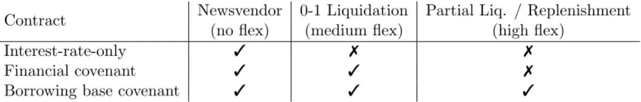
Contract Newsvendor 0-1 Liquidation Partial Liq. / Replenishment (no flex) (medium flex) (high flex)
Interest-rate-only 3 7 7
Financial covenant 3 3 7
Borrowing base covenant 3 3 3
Table 1: Optimal debt contracts required as a function of the firm’s operating flexibility. Check marks indicate feasibility of the contract incompletelyalleviating agency costs and restoring firm value. For instance, contracts that only include an interest rate are sufficient for a newsvendor (with no flexibility), but fail under added flexibility.
From a managerial perspective, our findings suggest that for debt contracts to be effective in practice, firms with enhanced flexibility and/or operating in better markets should be willing to abide by more and/or tighter covenants. This may seem counterintuitive to an operator, as (i) better markets may seem to be more “secure,” and (ii) covenants clearly restrict the firm’s operating discretion. Our model nevertheless predicts that optimally crafted covenants can fully mitigate agency issues, and are thus in a firm’s best interest. Managerial implications are further discussed in Section 7.1.
• Extending our model to capture how competition in the lending market can affect results, we examine the extreme case in which the lender acts as a monopoly. We find inventory-heavy firms to face more covenants as competition in the lending market wanes, and covenants to no longer be
sufficient to restore firm value.
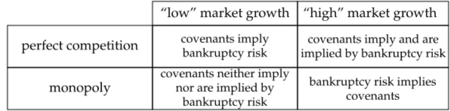
• Our model also shows the relationship between covenant inclusion and bankruptcy risk to be more subtle than previously reported in the literature, and critically dependent on competition in the lending market and residual growth in product demand. Table 2, which illustrates this relationship, shows that it is possible that covenants are included and the equilibrium probability of bankruptcy is zero. Also, it is possible in equilibrium that the risk of bankruptcy exists but covenants are not included in the debt contract. The table highlights, moreover, that covenants become more prevalent as competition in the lending market wanes or demand growth rate increases.
perfect competition
“low” market growth “high” market growth
covenants imply
bankruptcy risk implied by bankruptcy riskcovenants imply and are covenants neither imply
nor are implied by bankruptcy risk
bankruptcy risk implies covenants
monopoly
Table 2: Connection between bankruptcy risk and the inclusion of covenants.
The model extension for the monopolistic lending market is included in the Appendix B. Model limitations and future directions are summarized in Section 7.3.
Literature Review
Our work lies at the interface of operational and financial decision-making, an area pioneered by several recent papers. For instance, Xu and Birge (2004) and Dada and Hu (2008) extend the newsvendor model to include financing constraints, and show how these can affect the optimal order quantity or capacity choice. The focus here is on short-term financing in the form of trade credit or debt. We refer the reader to Kouvelis (2012) for a review of this literature. None of these papers consider a dynamic setting, where agency issues due to risk shifting could be relevant. Several papers in operations have discussed dynamic inventory decisions under capital constraints or leverage (e.g., Porteus 1972, Archibald et al. 2002, Gong et al. 2014), but without modeling strategic interactions or endogenizing debt contract terms. Boyabatlı et al. (2015) study the interplay of operational and financial flexility, albeit in a different context than ours.
Closer to our work, Boyabatlı and Toktay (2011) examine a firm’s optimal choice of flexible capacity under leverage in a static setting, finding that firms are more likely to choose flexible capacity when they use secured loans, and when they face less demand variability. Critically different from our model, flexibility does not create any agency issues in Boyabatlı and Toktay (2011), as it cannot be used to shift risk. To the best of our knowledge, only two papers in the operations literature examine the relationship between the agency costs of debt and flexibility.
Chod and Zhou (2014) study a newsvendor-style firm that first secures debt, and then chooses whether to invest in flexible or inflexible (but cheaper) resources. Risk shifting arises when the
latter option is chosen, as inflexible resources are “riskier” than flexible ones. Thus, in this static model, increased (resource) flexibility does not accentuate agency issues, but rather reduces them. In contrast, our emphasis is on studying the risk shifting potential that operating flexibility can introduce, which can only be captured in a dynamic setting. Finally, Chod (2015) study the role of trade credit in alleviating the agency costs of debt. The focus is on a newsvendor-style firm that first secures funding—through bank debt or trade credit—and then places orders for two types of products. The author shows how agency costs arise under (interest-only) debt financing, as the firm can order the “riskier” product once debt is in place. In contrast, when trade credit is provided by a single supplier who can directly contract upon the individual order quantities, agency costs are fully alleviated. While both Chod (2015) and the present paper discuss agency costs arising from operating flexibility, the papers differ dramatically in focus: the former looks at trade credit, while we examine the efficiency and optimal design of common financial contracts (with covenants).
On a broader level, our work is related to a large body of accounting, finance and economics literature that deals with agency issues and contractual incompleteness. Seminal works include Jensen and Meckling (1976), Myers (1977), Grossman and Hart (1986), and Aghion and Bolton (1992). Smith and Warner (1979) were the first to describe how covenants can be used to counter agency issues, whereas Leland (1994) argued how net worth covenants can mitigate agency issues occasioned by risk shifting. The literature on the role of covenants in alleviating agency and incompleteness is vast, and we make no attempt to survey it here—we refer the interested reader to Bolton and Dewatripont (2004), Tirole (2006), and references therein.
Several papers within this stream study agency costs derived from different types of flexibility, see, e.g., Childs et al. (2005), Leland (1998), Moyen (2007), Titman et al. (2004). The focus is on comparative statics to assess the directional impact of flexibility on such costs and/or numerical studies to quantify the magnitude of costs. Mello and Parsons (1992) and Manso (2008) study special forms of operating flexibility (captured through switching costs), with the latter deriving upper bounds on the agency costs. None of these papers look at the effectiveness of optimally designed covenants in alleviating agency costs, which is the primary focus of our paper.
Closer to our work, some recent papers focus on quantifying agency costs and covenant effec-tiveness. Gamba and Triantis (2014) compares the effectiveness of different types of covenants used in practice through a detailed numerical study, showing that covenants could restore anywhere from 0% to 90% of the firm value loss. Matvos (2013) develops a structural model to measure which types of covenants are most effective in practice, finding that covenant presence is essen-tial, but—once covenants are chosen—the benefits of “fine-tuning” them is marginal. In contrast, we find that significant firm value could be at stake if covenant tightness is not properly set (see Section 2). Neither of these papers looks at optimal covenant design. Berlin and Mester (1992),
Sridhar and Magee (1997) and Gˆarleanu and Zwiebel (2009) study the relation between optimal covenant design/tightness and renegotiation, which becomes important under information frictions. We instead study how to optimally design covenants in order to mitigate agency issues caused by (varying degrees of) operating flexibility, which, to the best of our knowledge, has not been looked at before. Moreover, the aforementioned papers do not focus on quantifying covenant effectiveness. In Section 7.2, we review several empirical papers in the literature studying covenant tightness, intensity, effectiveness that our work nuances and is either aligned with, or even counters.
2
Quantifying Agency Costs
Before introducing the modeling details and analysis, it will be useful to gain a better understanding of the magnitude of the effects discussed in the introduction. Are flexibility-driven agency costs a first order effect in our setting? To assess this, we first measure the potential value created by inventory flexibility, and then quantify how much of this value can be erased under leverage.
We rely on a base case newsvendor model, denoted by N, with a single selling season [0,2]. To introduce operating flexibility, we extend this model by splitting the selling season into two periods, [0,1] and [1,2], and in the spirit of Fisher et al. (2001), we allow an opportunity to adjust inventory in response to observed sales inbetween. We refer to this model as the “flexvendor.” As alluded to in the introduction, we study different degrees of the flexvendor’s flexibility in adjusting inventory. In this section, we consider the highest degree of flexibility, where the flexvendor can fully adjust inventory either by partial liquidation or replenishment, and study the following two variations:
F: a flexvendor with ample capital, who requires no debt financing.
Flev: a leveraged flexvendor, who primarily relies on debt financing through competitively-priced debt contracts that only include an interest rate.
The flexvendor model is rooted in reality, and motivated by the decision process faced by firms carrying inventory that depreciates in value over time. In particular, we are inspired by the case of Hewlett Packard (HP), which attempted to enter the tablet market in the summer of 2011, with two TouchPad devices (16GB and 32GB versions) that were based on HP’s proprietary webOS software. As of August 2011, the two devices retailed for $399.99 and $499.99, respectively (Rapaport and Tracer 2011). Over the course of the month, HP’s sales were extremely disappointing, while its competitors were rapidly gaining market share. It soon became apparent that HP’s software could become obsolete, unable to compete with the Apple and Android ecosystems. As a result, towards the end of August 2011, HP decided to completely liquidate its webOS line of tablets, at fire-sale prices. After some price experimentation, the retail liquidation prices were set at $249.99 and $299.99, respectively (Wikipedia 2011).
We rely on this example to calibrate the flexvendor’s operating parameters, namely prices and unit cost. As HP’s primary distribution channel was through wholesale to its retail partners
(e.g., Best Buy), we need estimates of HP’s wholesale prices during normal operations, and during liquidation. According to Damodaran (2015), retail consumer electronics margins averaged 18.38% in 2011. This implies tablet wholesale prices of around $338 (16GB) and $422 (32GB), during normal operations, and $211 (16GB) and $253 (32GB) during the liquidation. Furthermore, HP’s unit costs—including parts and labor—were estimated at around $306.15 (16GB) and $328.15 (32GB), (Wikipedia 2011). Averaging across the two devices, we obtain an average unit cost of around 83% of wholesale, and an average liquidation price of around 61% of wholesale.
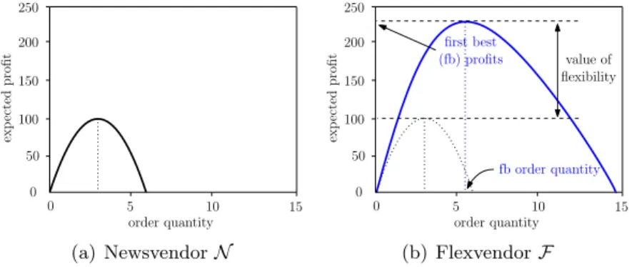
Accordingly, we normalize the flexvendor selling price to 1, and set the unit ordering cost to 0.83 (in both periods) and the liquidation value to 0.61 at time 1. To capture the webOS technological obsolescence, there is no salvage value at time 2. Further, we assume first period demand is uniformly distributed between [0,10], and the second period demand—conditioned on the first period realized demand beingd1—is uniformly distributed in [0,2d1]. Flev uses equity of 0.2, so that the purchase is primarily financed by debt. The profits are also normalized to ease exposition, such that the expected profits ofN are set at 100, see Figure 1(a).
Comparing the newsvendorN in Figure 1(a) to the flexvendorF in Figure 1(b) highlights the value of inventory flexibility: the flexvendor extracts profits of 235, a 135% increase compared to the newsvendor. This also represents the “first best” outcome for the flexvendor, i.e., the total profits or firm value achievable with flexibility, and without any financial frictions.
0 5 10 15 100 0 200 order quantity exp ected profit 150 50 250 (a) NewsvendorN value of flexibility fb order quantity first best (fb) profits 0 5 10 15 100 0 200 order quantity exp ected profit 150 50 250 (b) FlexvendorF
Figure 1: The value of operating flexibility: (a) Newsvendor vs. (b) Flexvendor
Introducing debt financing leads to agency issues, as the leveraged flexvendor—shielded by lim-ited liability—can use his additional operating flexibility to adjust the inventory level in risky ways, e.g., by carrying too much inventory into the second period (this intuition is formalized in Section 4). This leads to some rather striking results. If debtholders do not anticipate this risk shifting po-tential, the leveraged flexvendor could expropriate wealth from them, and beat first best, as shown in Figure 2(a). Under equilibrium pricing, debtholders fully anticipate risk shifting and increase borrowing rates in response, which introduces agency costs, as shown in Figure 2(b). Consequently, the leveraged flexvendor achieves profits of 160, which are 32% lower than the flexvendor’s first best. This loss is substantial, suggesting that flexibility-driven agency costs can be a dominant
effect in our setting,3 potentially shaping operations strategy. For instance, consider the situation where the newsvendor would need to invest 100 to obtain the reordering/liquidation flexibility of the flexvendor. In the absence of financial frictions, such an investment would be fully justified, yielding a net benefit of 135−100 = 35. However, under financial frictions, the net benefit becomes 60−100 =−40, rendering the investment unattractive.
wealth extraction 0 5 10 15 100 0 200 order quantity exp ected profit 150 50 250
(a) Risk shifting example
value lost due to agency costs (32%) sb order quantity second best (sb) profits 0 5 10 15 100 0 200 order quantity exp ected profit 150 50 250
(b) Agency costs created
Figure 2: How a leveraged flexvendor could shift risk to extract wealth from non-anticipating debtholders (a), and how agency costs are created when debtholders anticipate this behavior in equilibrium (b), in the context of interest-only debt contracts.
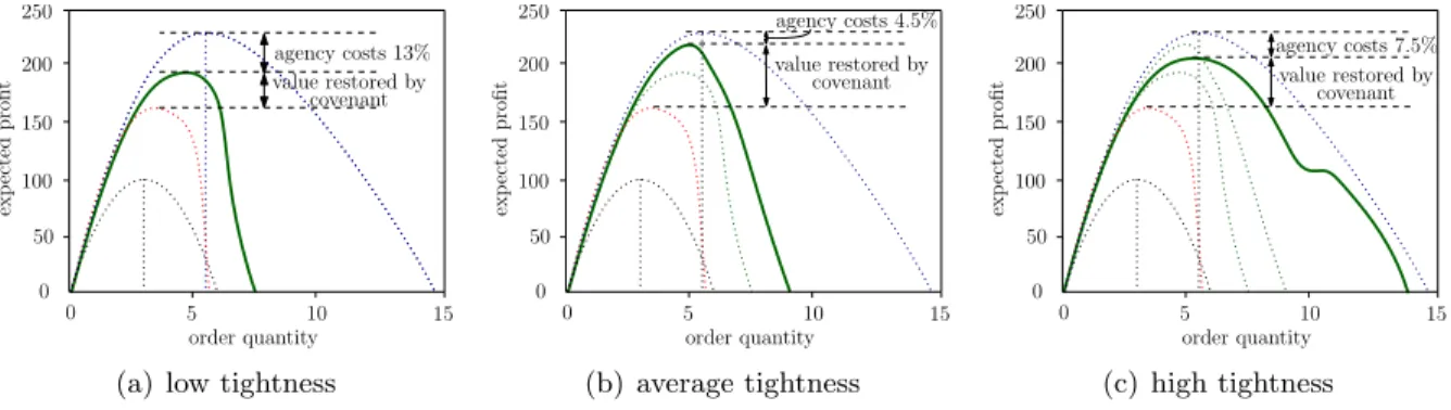
To evaluate the potential of covenants in alleviating agency costs, we now consider the case where the debt contract for the leveraged flexvendor includes a simple financial covenant of varying tightness, evaluated between the two periods. In particular, the covenant requires that the cash generated from sales in the first period meet a minimum threshold. The covenant becomes tighter as the required threshold increases. Upon covenant violation, the decision rights are transferred to the debtholders. Figure 3 illustrates the effectiveness of a covenant with (a) low, (b) medium or (c) high tightness in mitigating the value losses. It is interesting to note that the three covenants reduce agency costs to (a) 13%, (b) 4.5%, and (c) 7.5%, respectively, so that effectiveness is non-monotonic in covenant tightness. The intuition behind this is that if the covenant is too loose, risk shifting activities are not adequately restricted. However, if the covenant is too tight, then the debtholders essentially control the firm after the first period, and take decisions that are also inefficient. We discuss this extensively in Section 5.
While this simple example sets the stage, it leaves much unanswered: How effective are financial covenants in mitigating flexibility-driven agency costs and restoring firm value? Is one covenant enough, or are more needed? How should the covenant intensity and tightness be structured as a function of the product (price, margin, salvage), the market (demand growth), and the firm’s operating capabilities (reordering and liquidation options)? The rest of the paper seeks answers to
3We conducted several robustness checks, by varying all parameters in this model, and the magnitude of the effect
persisted. We note that these costs are larger than values reported in other studies. For instance, Chod (2015) reports agency costs of less than 8% in a single-period inventory model, while Gamba and Triantis (2014) report costs as large as 18% (albeit in a very different model specification).
agency costs 13% value restored by covenant 0 5 10 15 100 0 200 order quantity exp ected profit 150 50 250
(a) low tightness
agency costs 4.5% value restored by covenant 0 5 10 15 100 0 200 order quantity exp ected profit 150 50 250 (b) average tightness agency costs 7.5% value restored by covenant 0 5 10 15 100 0 200 order quantity exp ected profit 150 50 250 (c) high tightness
Figure 3: Quantifying how much value covenants can restore for the leveraged flexvendor, as a function of tightness.
these questions.
3
Model
We introduce the flexvendor model by considering a newsvendor who has an early exit option, i.e., an intermediate time-step at which all remaining inventory can be liquidated, before fully depreciating (we return to study the flexvendor with replenishment flexibility in Section 6).
3.1 Flexvendor With a Liquidation Option
We consider a setting in which a firm can purchase a single type of product at timet= 0, at unit costc >0. The number of units to purchase is denoted byq; full payment ofc qis due upon delivery of the purchased units, which occurs with zero lead time. There are two selling periods, over which products are sold at pricep= 1> c. Att= 1, the first period random demandD1 is realized, and fulfilled to the largest extent possible from the initial inventory ofq units. We assume thatD1 has non-negative support, cumulative distribution function (c.d.f.) F1 and probability density function (p.d.f.) f1, and denote a realization withd1.
At this point, a participating firm faces two options: it can either liquidate (e.g., salvage) the remaining inventory (q−d1)+ (if any) at unit price s < c and exit the market immediately, or continue operating for a second selling period. The decision to continue or liquidate, denoted by
`∈ {0,1}, is based on the information set att= 1, which consists of the realized demand d1. If the firm chooses to continue, i.e., ` = 0, the second period demand D2 is realized and fulfilled at t = 2, to the largest extent possible. We assume that D2 depends on d1, specifically,
D2|{D1 = d1} = M2−1d1Z, where Z is a non-negative random variable with unit mean, and
M >1 is a parameter determining thedemand growth rate, ormarket strength. In particular, since
E[D2|D1 =d1] = M2−1d1, demand is projected to increase if M ≥ 3, and decrease otherwise. We refer to these cases as follows.
Unmet demand is lost without any penalty in both periods, and any remaining inventory is dis-posed of, without salvage value or cost.4 For simplicity, we assume a zero discount rate throughout the analysis. The value extracted from such a market under an initial orderq is thus given by the firm’s expected profit,
V(q) =ED1 min(D1, q) + max `∈{0,1} n `·s(q−D1)++ (1−`)·ED2|D1 h min D2,(q−D1)+io , (1)
and the firm chooses q at t = 0 so as to maximize V(q). Let Vfb def= maxq≥0V(q) denote the optimal extracted value, andqfb denote the associated optimal order quantity, henceforth referred to asfirst best.
3.2 Leveraged Flexvendor
A firm (e.g., a retailer)Roperates in the setting described above. When the firm’s initial capitalx0 is insufficient to cover the inventory costcq, it can obtain debt financing from aperfectly competitive
lending market. More precisely, a bankB(“she”) can extend a loan for the amountw def= (cq−x0)+,5 under a contract with the following (T)erms and (C)ontingencies.
[T1] (Interest rate and repayment) Payment of principal plus interest charges (at rater) is due at
t= 2. For ease of exposition, we considerR= 1 +r in the remainder of the paper, and refer to it simply as the interest rate. The amount due at t= 2 is then Rw.
[T2] (Collateral and withdrawal) The bank obtainsperfect security interest in the entire inventory (to be) purchased by the firm. All cash generated by selling the inventory is remitted to a lockbox account controlled by the bank, and the firm is unable to access the funds until the entire loan proceeds Rw are fully repaid, at t= 2. In other words, the lockbox account has a zero withdrawal limit.
[C1] (Financial covenant) In period t= 1, the firm’s cash flow min(d1, q) is required to exceed a thresholdδ. Failure to abide by the covenant is considered an event of default, which gives the bank full control rights, as well as the ability to request immediate repayment of all due principal plus interest,Rw.
[C2] (Borrowing base covenant) In period t= 1, the firm’s borrowing base is calculated using an advance rate of 1 for cash andα∈[0,1) for inventory, and is thus equal to min(d1, q)+α s(q−
d1)+. The borrowing base is required to exceed a thresholdβ, and as with [C1], failure to conform triggers an event of default, and carries the same repercussions.
4The assumption of zero salvage att= 2 simplifies exposition, without affecting our structural results and insights. 5We implicitly assume that all available equity is used to purchase the inventory att= 0. Absent other
All contracts we consider include terms [T1-2]. We denote the set of contracts that include no contingencies by K∅, and refer to such contracts as interest-rate-only contracts. Similarly, let KF
be the set of contracts that include a financial covenant [C1] only, andKB the set of contracts that
include a borrowing base covenant [C2] only. It is worth noting that a borrowing base covenant is more general than a financial (i.e., cash flow based) covenant, since the latter can always be replicated through the former by takingα= 0 and β =δ. As such,K∅ ⊂KF⊂KB.
We consider separate model specifications, in which contracts are chosen from eitherK∅,KF or KB. To simplify notation, we denote any contract withκ.
3.2.1 Timing of Events
We study the game under perfect and symmetric information between the two players, R and B. Att= 0, the firm chooses an order quantityq, and the bank chooses the terms (and contingencies) in the loan contract κ.
Att= 1, demandd1is revealed to both players and fulfilled, generating a cash flow of min(d1, q) for the firm. As described above, the firm has the option of continuing operating for a second selling period, or liquidating any leftover inventory at s and exiting the market. If the latter option is chosen, the firm uses generated cash flow and liquidation revenues, equal to min(d1, q) +s(q−d1)+, to repay its debt of Rw. Let `R : R×R → {0,1} denote the firm’s liquidation policy, with `R(q, d1) = 1 if and only if the firm liquidates when the initial inventory isq, and D1 =d1.
If the firm chooses to continue operating and the contract includes a covenant, then the bank evaluates the covenant requirement. If it is breached, the bank has the option of forcing liquidation in order to secure full payment of the debt. In case the bank exercises this option, she seizes remaining inventory and liquidates it at unit price s. All proceeds from sales and liquidation are first used towards debt servicing. If the bank is made whole, the remaining revenues are returned to the firm. Similar to our previous notation, let `B :R×R→ {0,1}denote the liquidation policy
of the bank. Note that, unless a covenant is included in the contract and it is breached, the bank does not have any right to influence the liquidation/continuation decision.
When the firm chooses to continue and the bank does not force liquidation, the second period demandD2is realized and filled to the largest extent possible. Att= 2, the generated sales revenues from the two periods are first used to repay the debt Rw, and the firm keeps any remaining cash and exits the market.
In this setting, the firm’s and the bank’s cash flows at the end of the game under the liquidation event6 L (irrespective of the party choosing that option) and continuation event C def= Lc are
6More formally,
L def= {`R(q, D1) = 1} ∪V ∩ {`B(q, D1) = 1} , whereVis the event corresponding to a covenant
breach, i.e.,V def=
respectively given by
XR,L(q, D1) = min(D1, q) +s(q−D1)+−Rw+, XR,C(q, D1, D2) = (min(D1+D2, q)−Rw)+,
XB,L(q, D1) = minRw, min(D1, q) +s(q−D1)+ , XB,C(q, D1, D2) = minRw, min(D1+D2, q) . For the firm, both expressions have a floor at 0, reflecting its limited liability. For clarity, we refer to the game at t = 1 that determines whether L orC occurs as subgame S. The pure subgame perfect equilibrium actions can be characterized via backward induction. When κ∈K∅, the game
only entails choices by the firm. Whenκ∈KF∪KB, the outcome of the subgameScan be viewed
as a Stackelberg game, with the firm leading by choosing `R and the bank following by choosing
`B (see Figure 4(b)).
At t= 0, the expected profits of the two players can then be compactly expressed as
πR(q, κ) =EXR,L(q, D1)1{L}+XR,C(q, D1, D2)1{C}−x0,
πB(q, κ) =EXB,L(q, D1)1{L}+XB,C(q, D1, D2)1{C}−w,
where 1 is an indicator function. The firm chooses the order quantity q so as to maximize its expected profit πR(q, κ), and the bank chooses the debt contract terms κ so as to break even in expectation, i.e., πB(q, κ) = 0. The sequence of all events is illustrated in Figure 4.
t= 0 t= 1 t= 2
demand revealed & contract R,B D L ... | {z } ...| {z }...| {z } subgameSwith outcomesC orL demand revealed C d2 D S {πR;πB} {πR;πB} d1 q,κ signed
(a) Game under perfect competition
violation R `R= 1 `R= 0 R B `B= 0 `B= 1 ... | {z } liquidation/ continuation decisions ... | {z } covenant evaluation L C C
⇔
L C S `R= 0 L no violation (b) SubgameSFigure 4: Game under perfect competition and subgameSforκ∈KF∪KB(R=Firm,B=Bank,D=Demand).
Assumptions for Analysis
For the sake of analytical tractability, we also introduce the following simplifying assumptions. We relax these in Section 6.
Assumption 1. The random variable Z that drives second period demand follows a two-point distribution, taking values0 and2 with equal probability.
The two-point distribution introduces an adverse (D2 = 0, for Z = 0) and a favorable scenario (D2 = (M −1)d1, for Z = 2) for the second period demand. Our choices of zero demand in the adverse scenario and equally likely scenarios allow us to ease exposition, without affecting the validity of the structural results.
Under Assumption 1, the probability of selling a unit of inventory over the second period is at most 1/2, and the corresponding expected revenues are at most 1/2 as well, since the selling price is 1. On the other hand, liquidation yields revenues of s per unit att = 1. It is easy to see that, unless s < 1/2, the firm would never prefer to continue in the second period, but rather behave as a classical newsvendor who sells over one period and then liquidates (or salvages) his leftover inventory. To circumvent this degeneracy, we introduce the following assumption:
Assumption 2. The liquidation price satisfies s <1/2.
It is hardly surprising that an upper bound on the value of s is needed to eliminate trivial cases when liquidation is always preferred.
3.3 Discussion of Modeling Assumptions
Business cycle. Our model extends the classical newsvendor framework by providing a liquidation option at an intermediate point. This can correspond to a discontinuation of a division or product, or a going out of business sale (Craig and Raman 2013). Paralleling the standard “salvaging” assumption in the newsvendor setup, we assume that the entire leftover inventory at t = 1 can be liquidated at a pricesthat is a-priori known, and independent of the quantity and first period demand. While simplistic,7 this assumption adequately captures the mechanisms at play in our setting, and becomes even more sensible when the bank is also endowed with a liquidation option. In practice, such liquidations are typically contracted to an external party, such as Gordon Brothers Group, Hilco Global, ES Group, etc. Such a liquidation house provides binding inventory appraisals upfront (i.e., in period t= 0), and, in case of liquidation, purchases the entire inventory at a fixed per-unit price, which reflects a pre-determined haircut on the original appraised value. Thus, any remaining liquidation risk beyond this haircut is essentially transferred to the liquidation house (see Craig and Raman 2013 for more details).
Demand distribution. Requiring D1 and D2 to be correlated is standard in the literature (Fisher and Raman 1996). Our assumption of a discrete second period demand distribution has been widely used in the literature in similar multi-period game-theoretic models (e.g., see Bolton and Dewatripont 2004 and references in our literature review in Section 1). Despite its simplicity, the
7Cachon and Kok (2007) recognize that the effective salvaging price depends on remaining inventory, and discuss
appropriate ways for estimating this price. There is also an extensive literature in revenue management concerned with optimal markdown, the practice of dynamically adjusting prices for remaining inventory at the end of a selling season, for the purpose of freeing valuable shelf space (see, e.g., Talluri and Van Ryzin 2004 and Phillips 2005).
two-point distribution is sufficiently rich to capture the main trade-offs driving the players’ dynamic decisions, and the results derived are robust, as discussed in Section 6 and Section C.1.
Exogenous retail price. We note that the flexvendor in our model is assumed to be price-taking, as in the classical newsvendor setting.
Collateral. Assuming the loan to be secured allows us to abstract away from potential complexities related to the bank’s seniority in the capital structure.
No loan limit. In our model, given that the interest rate is determined endogenously, a loan limit would be superfluous and is thus omitted. This is standard in the finance and the OM literatures (Boyabatlı and Toktay 2011, Gˆarleanu and Zwiebel 2009, Myers 1977, Xu and Birge 2004).
No cash diversion/dividends. The presence of a lockbox account and the implicit assumption of no dividend payment are both common requirements in loan agreements (see Chapter 7 of Hilson 2013, pages 14 and 19). In our model, this allows abstracting away any additional agency issues related to cash diversion, and focusing on agency issues exclusively due to operating flexibility.
No additional financing. Allowing the firm no access to other external capital (e.g., by new equity or debt issuance) during the life of the contract is standard in the literature (see, e.g., Chod and Zhou 2014, Gˆarleanu and Zwiebel 2009, Myers 1977, Xu and Birge 2004). This allows focusing on the relationship between the two agents.
Contingencies. Since the goal of our paper is to quantify the effectiveness of simple and practical covenants in alleviating agency issues, the debt contracts we consider only include financial or borrowing base covenants. Together with pricing grids, these are the most commonly used forms of contingencies in practice, as documented by numerous empirical papers (Roberts and Sufi 2009a).
Financial covenant. Financial covenants involve various metrics, such as cash-flow-to-debt ratio, net worth, interest rate coverage, EBIT to interest ratio, etc. (see, e.g., Dichev and Skinner 2002, Roberts and Sufi 2009b, and pages 2-4 in Chapter 7 of Hilson 2013). In our base model, it turns out that all such covenants translate into a minimum threshold requirement on the cash flow or, equivalently, on the first period demand d1 (note that the covenant can never be breached upon stock-out).8 The choice of a particular type of financial covenant is therefore without loss of generality, so that we henceforth base our analysis and discussion on a minimum cash flow thresholdδ that controls the covenant tightness. Finally, entitlement to immediate debt payment upon a covenant breach is routinely included in contracts (see page 17 in Chapter 7 of Hilson 2013).
Borrowing base covenant. Theborrowing baseis the value assigned to the borrower’s pledged assets, calculated by applying particular advance rates against each type of collateral. These rates (i.e.,
8For instance, consider a covenant requiring the net worth to be higher than a thresholdτ. Ford
1 < q, debt at
t= 1 is equal toRw, and equity is equal tod1+s(q−d1). The covenant then equivalently requires demand to be
“hair-cuts”) are chosen by the lender as additional risk controls, reflecting the riskiness of each asset class. Our assumption that cash and inventory have advance rates of 1 and α, respectively, is consistent with common practice, where accounts receivable advance rates are often 90%-100%, while inventory rates range from 50% to 90% (Buzacott and Zhang 2004, CH 2014). Most secured contracts include contingencies requiring the borrowing base to exceed the size of the outstanding debt throughout the life of the loan. We note that the covenant used in our model is slightly more general, by requiring the borrowing base att= 1 to exceed a valueβ, which is not necessarily equal to the outstanding debt. We retain the terminology of “borrowing base covenant” for simplicity of exposition. β controls the tightness of the covenant. A borrowing base requirement att= 0 would essentially be equivalent to a loan limit, which is superfluous as per our discussion above.
Bankruptcy costs and procedures. In the event of default, we only consider Chapter 7 bankruptcy (“liquidation”), but not Chapter 11 (“reorganization”), which would involve having to model the renegotiation process between the parties. Note also that, in view of our assumption of perfect and symmetric information, a renegotiation process would be superfluous (see Gˆarleanu and Zwiebel 2009). We also ignore bankruptcy costs. For a discussion on the effects of non-zero bankruptcy costs and reorganization, we refer the reader to Birge and Yang (2013) and Birge et al. (2015).
4
Liquidation Policies
We analyze the players’ optimal liquidation policies in subgame S, at the intermediate time t= 1. To provide a meaningful comparison, we start by deriving the first best policy.
4.1 First Best Liquidation Policy
When the order quantity is q, and the first period demand realization is D1 = d, the first best policy can be readily derived as the optimal liquidation decision` in (1).
Lemma 1 (First Best). The first best liquidation policy is a threshold one,
`fb(q, d) =1{d < dfb(q)}, where dfb(q) def= M−sq1 2 +s
.
Such a threshold policy is consistent with intuition and hardly surprising. Many studies dealing with dynamic decisions under debt either de facto assume or derive such policies as optimal (see, e.g., Babich and Sobel 2004, Gigler et al. 2009, Hart and Moore 1998, Morellec 2001, Swinney and Netessine 2009). Furthermore, as one might intuitively expect, the threshold dfb is increasing in q and s and decreasing in M, confirming that the propensity to liquidate increases with order quantity and liquidation value, but decreases with the second period market strength.
4.2 Leveraged Firm
Under debt, the firm’s liquidation decisions generally depart from first best. The optimal policy turns out to critically depend on whether the order quantity q exceeds a particular threshold qD, given by qD def= Rx0 Rc− 2s M−1+2s ifM ≥M˜ and s < s1 D, Rx0 Rc− sM M+s−1 ifM <M˜ and s < s2 D, ∞ otherwise, (2) where ˜M def= 2(1−s), s1 D def = Rc2(1(M−−Rc1)),s2 D def
= RcM(M−−Rc1). We introduce the following definitions.
Definition 2. When q > qD (q ≤qD), we say that the firm is (not) sufficiently leveraged.
Definition 3. When M <M˜ (M ≥M˜), we say that the market is (not) rapidly shrinking.
The first moniker is intuitive, since largerq is tantamount to a larger debt load. Note that whether this condition holds critically depends on market parameters. In particular, firms are never suffi-ciently leveraged when inventory does not depreciate too rapidly (i.e.,sexceeds some critical value), and an important distinction is drawn depending on whether markets are “rapidly shrinking,” as captured in the second definition. Since ˜M <2, a rapidly shrinking market is reflective of a second period expected demand considerably below the first period realized demand, which is consistent with (and stronger than) our earlier condition for a “shrinking market,”M <3.
With these definitions, we now characterize the liquidation policy of a leveraged firm.
Lemma 2 (Leveraged Firm). In equilibrium,
(a) a firm that is not sufficiently leveraged follows the first best liquidation policy, i.e., `R(q, d) =
`fb(q, d).
(b) a firm that is sufficiently leveraged and operates in a market that is not rapidly shrinking follows a threshold liquidation policy: `R(q, d) =1d < dR(q) .
(c) a firm that is sufficiently leveraged and operates in a market that is rapidly shrinking follows a non-threshold policy: `R(q, d) =1 n d∈0, RwM ∪ dR(q), dfb(q)o, where dR(q) def= Rw M , ifM = ˜M , maxM2sq−2(1−Rw−s),RwM otherwise.
It is worth noting that a leveraged firm follows the same policy in both the upper and the lower node of subgame S, i.e., its policy is unaffected by a covenant breach. This is intuitive, since its
own policy becomes irrelevant when the breach happens, so that the optimal policy in equilibrium is the same as when the covenant is not breached.
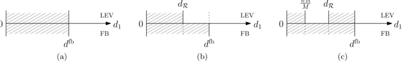
Lemma 2 is summarized in Figure 5. Note that a firm’s behavior critically depends on whether it is sufficiently leveraged, and on whether the market is rapidly shrinking or not. As intuition would dictate, under small enough debt levels, a leveraged firm acts as if the entire order were funded using its own equity (see Figure 5(a)). However, as leverage increases, the policy starts to deviate substantially. dfb d1 FB 0 LEV (a) dR dfb d1 0 LEV FB (b) dR dfb d1 wR M 0 LEV FB (c)
Figure 5: Firm’s optimal liquidation policy as a function of realized demandd1. The shaded area denotes a preference
for liquidation at t= 1. The policy above the horizontal axis corresponds to a leveraged firm, when it is (a) not sufficiently leveraged, or sufficiently leveraged in a market that is (b) not rapidly shrinking or (c) rapidly shrinking. For comparison, the first best policy is depicted below the axis.
When the market is not rapidly shrinking, a sufficiently leveraged firm still follows a threshold policy, but starts liquidating less often than first best, see Figure 5(b). In fact, the new threshold
dR(q) is not only lower than dfb(q), but also increases in q at a lower rate, implying that the discrepancy in policies becomes even more pronounced as leverage increases.
Surprisingly, a sufficiently leveraged firm operating in a rapidly shrinking market entirely de-parts from threshold policies, see Figure 5(c). To understand this behavior, note that market conditions in this case are particularly dire, as bleak second period prospects are compounded by a rapidly depreciating inventory value (s < s2D). At intermediate sales levels wRM < d < dR(q), the latter effect takes precedence, as liquidating (a relatively large) inventory would mean imme-diate insolvency or extremely low profits for a leveraged firm, while continuing could yield hope of high(er) profit if the high demand scenario materializes. As before, it is important to note that a leveraged firm liquidates less often than first best. However, the disagreement here occurs at intermediate sales levels, where the first best policy liquidates so as to recover a higher total asset value, while a leveraged firm gambles on continuation. We note that non-threshold policies are not a by-product of our assumptions, and they persist under considerably more general settings – see the discussion in Section C.1 of the Appendix.
The critical threshold qD can also be connected with the existence of bankruptcy risk in the debt agreement, as summarized in the following result.
Lemma 3 (Sufficient leverage and bankruptcy). Under either the first best or the leveraged firm’s liquidation policy, q > qD is
(i) a necessary and sufficient condition for bankruptcy risk in non-shrinking markets, and (ii) a sufficient (but not necessary) condition for bankruptcy risk in shrinking markets.
The result implies that sufficiently leveraged firms always induce bankruptcy risk, and, in fact, the former phenomenon is actually synonymous with the latter in non-shrinking markets. Since such markets may be quite natural in practice, this fact bears very relevant implications for our analysis, suggesting that risky lending agreements of the type examined here are likely to involve sufficiently leveraged firms, whose liquidation policies depart from first best. Interestingly, this is not necessarily the case in shrinking markets. Note that the distinction between the two regimes is given by our earlier definition of shrinking markets (i.e., M ≷ 3), instead of rapidly shrinking markets (i.e.,M ≷M˜).
4.3 Bank
We next analyze the bank’s optimal liquidation policy in subgameS (see Figure 4(b)).
Lemma 4 (Bank’s liquidation policy). In equilibrium, the bank follows the threshold liquidation policy `B(q, d1) =1
d1 < dB(q) , unless the collateral value depreciates very rapidly (s < sB) and
the firm is highly leveraged (q > qB), in which case she follows the non-threshold policy `B(q, d1) = 1 n d1 ∈0, dfb(q)∪ Rw−1−22sqs, dB(q)o,where qB def= cRR(M(M−−1+21+2s)s−)x20M s,sB def = (2(MM−−cR1)cR), anddB(q) def= Rw.
The result suggests that, barring a particular case, the bank follows a threshold liquidation policy, with a threshold dB(q) that increases in q, R and c, and decreases in x0. It is important to note that the bank’s own liquidation preferences are also not efficient in general. In particular, it can be checked that `B(q, d1)≥`fb(q, d1), reflecting the bank’s preference for conservative actions that result in more liquidation than first best.
Interestingly, the bank also departs from a threshold policy, under similar conditions as the firm, i.e., low liquidation value and high leverage. Here, when the realized sales are low (d1 < Rw1−−22sqs), it can be checked that the firm is bankrupt, and the bank is set to seize all its assets, either at
t= 1 or at t= 2. As such, the bank effectively becomes the owner and operator of the inventory, and prefers to follow the first best policy, liquidating below the threshold dfb(q), and continuing otherwise.
While in this paper we assumed perfect and symmetric information, it is nonetheless interesting to briefly consider a setting where the bank is unable to directly observe the firm’s first period sales. In such a case, when optimal, the bank’s non-threshold liquidation policy might induce a firm with sales above Rw−1−22sqs, but below dB, to underreport the sales, so as to avoid liquidation.9
9It can be checked that such a firm would prefer continuation to liquidation, and may thus choose to report sales
This effect has already been documented in the context of debt-service renegotiation, where a borrower in default may overstate their debt service abatement in order to obtain better terms from the lender. Specifically, Bourgeon and Dionne (2013) find that asymmetric information about liquidation value might induce firms with high values to act as firms with lower values. In our case, sales underreporting would not be driven only by information asymmetry, but also by the players’ operational preferences. Similar to Bourgeon and Dionne (2013), our model also suggests that this behavior would be more likely in markets where liquidation values are low and leverage is high.
4.4 Liquidation Conflict
To understand how tension between the players may arise, we now compare their optimal liquidation policies, and identify the circumstances under which they are in (dis)agreement. To this end, note that the firm would never prefer liquidating its inventory if this action lead to insolvency. As such, whenever the firm prefers liquidation, the bank is always made whole, and the two players are in agreement. When the firm prefers to continue, however, it is possible that the bank might prefer liquidation. This prompts us to introduce the following definition.
Definition 4. We define the disagreement region D as the set of first period demand realizations for which the liquidation preferences of the two players are misaligned. More formally,
D def= n
d≥0|XR,L(q, d)<E[XR,C(q, d, D2)|D1 =d]andXB,L(q, d)>E[XB,C(q, d, D2)|D1=d]
o . Whenever D6=∅, we say that liquidation conflict exists between the two players.
Liquidation conflict here is a direct manifestation of agency issues,10driven by the shareholder-debtholder conflict of interest (Jensen and Meckling 1976, Myers 1977, Smith and Warner 1979). Intuitively, by continuing, the firm (shareholder) has limited downside and potentially large upside, due to its leverage. It is thus effectively shifting risk to the bank (debtholder). On the contrary, the bank may prefer liquidation, so as not to expose the collateral to further potential depreciation. Note that the existence and the extent of liquidation conflict critically depend on the firm’s order quantityq and market parameters. To this end, our next result precisely characterizes the disagree-ment region, showing that it is always a (possibly empty) interval of demand values, intrinsically related to whether a firm is sufficiently leveraged.
Lemma 5 (Liquidation conflict). In equilibrium, liquidation conflict arises if and only if the firm
10We note that agency issues may exist between the two players in other forms, as well, e.g., concerning the choice
of initial order quantityq(see, e.g., Buzacott and Zhang 2004). We use the term “liquidation conflict” to completely isolate the effect, and pinpoint that it is related to dynamic inventory decisions, i.e., liquidation policies.
is sufficiently leveraged. More precisely, D= ∅, ifq ≤qD, d(q), d(q), otherwise, where d(q) def= maxdR(q),Rw1−−22ssq ifM ≥M ,˜ maxRwM ,Rw1−−22ssq otherwise, and d(q) def= dB(q) ifM ≥M ,˜ min (dB(q), dR(q)) otherwise. Moreover, d(q)−d(q) is increasing in q.
The result shows that the two players are in complete agreement, i.e., D = ∅, when the firm is
not sufficiently leveraged. Otherwise, liquidation conflict always arises, at intermediate levels of sales, d(q), d(q). This is quite intuitive, since for low (high) enough sales, both players agree that the optimal action is to liquidate (continue). Furthermore, there is increasing conflict as leverage increases, and, ceteris paribus, conflict is more likely as the market strength M, the interest rate
R or the per-unit costc increase, or as the firm’s initial capitalx0 decreases.
In view of our earlier results, liquidation conflict arises exactly when leveraged firms deviate from first best. More interestingly, note that while liquidation conflict always arises in the presence of bankruptcy risk in non-shrinking markets, that is not necessarily the case if the market is shrinking: strictly higher leverage may be required to generate liquidation conflict, than to result in bankruptcy risk (see Lemma 3).
5
Flexibility-driven Agency Costs and Covenant Effectiveness
The liquidation conflict identified above could potentially give rise to agency costs. To formalize this, consider a firm desiring to follow the first best actions, and thus orderqfb. Since a debt contract signed att= 0 cannot explicitly bind the firm to follow a particular operational policy att= 1,11 once the debt is in place, the (now leveraged) firm would actually follow the liquidation policy `R
in equilibrium, which generally differs from the first best policy`fb, as discussed in Lemma 2. By rationally anticipating this risk shifting behavior att= 1, the bank would charge a higher interest rate, generating financing costs that could be large enough to induce the firm to reduce its initial debt burden and order quantity. This could lead to a value loss, with the firm’s expected profits being lower than the maximum possible value ofVfb.
Liquidation conflict and its associated agency costs shed light on why covenants may be useful. When there is disagreement concerning the liquidation decision, an appropriately crafted covenant
11This is consistent with typical assumptions in the literature on incomplete contracts (see, e.g., Aghion and
Bolton 1992, Hart and Moore 1998), as well as with observed practice. Contracts that seek to prescribe actions or payments for every possible contingency would be overly complex, and would also not be enforceable ex-post in a court (Gˆarleanu and Zwiebel 2009, Hilson 2013, Tirole 2006).
would offer the lender protection through the transfer of control rights. To see this, note that when the firm’s order quantity q results in liquidation conflict, i.e., D 6= ∅, the inclusion of a financial
covenant with a cash flow threshold δ ∈ D would give the bank the right to force liquidation at t= 1 wheneverd1 ∈(d(q), δ), an action that would be optimal for her, but not for the firm. This added protection would enable the bank to lower the interest rate, and thus the agency costs of debt could be reduced. Would overly tight covenants, warranting ever decreasing interest rates, then fully alleviate agency costs? The answer is clearly no, as in that case the bank’s liquidation preferences would be enforced, which we have also argued to be inefficient (Section 4.3).
This leads to the central question addressed in our paper: How effective are simple covenants in mitigating agency costs, i.e., how much value can they restore?
Theoretically, state-contingent control transfer mechanisms such as covenants could conceivably fully alleviate agency costs as long as they ensure that, in any state of the world, control rights lie with a player who prefers to follow the first best action in that particular state. In our setting, it is entirely unclear whether such a mechanism is possible, particularly when limiting attention to the simple (financial or borrowing base) covenants encountered in practice. Worse, the players’
non-threshold policies might further undermine the effectiveness of such simple covenants.
To study these issues, we now formally define the agency costs of debt. To simplify contract notation, we omit the interest rateR, as it is always determined endogenously as a function of all other parameters and decisions, so that the bank breaks even.
For a contract κ, let VR(κ) denote the maximum expected profit achievable by the firm, i.e.,
VR(κ) def= maximize πR(q, κ) subject to q ≥0
πB(q, κ) = 0.
(3)
The associated agency costs correspond to the relative value loss compared with the optimal ex-tracted value under the first best actions, i.e.,
A(κ) def= V fb−V
R(κ)
Vfb . (4)
In equilibrium, when contracts are optimally chosen from a particular set K∈ {K∅,KF,KB}, the
resulting agency costs are given by infκ∈KA(κ). The lower the equilibrium agency costs are, the more effective the set of contractsKis in alleviating agency issues.
In the remainder of the analysis, let q? and `? denote the equilibrium quantity and liquidation
5.1 Interest-Rate-Only Contracts
The following result confirms that interest-rate-only contracts generally fail to alleviate agency issues, and lead to an equilibrium where firms with low capital under-order relative to first best.
Theorem 1. Under interest-rate-only contracts,
(i) if x0 ≥x˜0, infκ∈K∅A(κ) = 0. In particular, there are no agency costs, q? =qfb, and `? =`fb.
(ii) if x0<x˜0, infκ∈K∅A(κ)>0. In particular, agency costs persist, q
? < qfb, and`? =`
R≤`fb.
Here, ˜x0 is a threshold that is strictly lower than c qfb and depends only on the market param-eters M, c, s, and F1 (for an explicit characterization, see the proof of the theorem). The result confirms that, under interest-rate-only contracts, firms with low initial capital will always be faced with agency costs, as their high leverage coupled with the inability to relinquish control rights will always make them “too risky” for the lender. Put differently, such firms will always be unable to harness the full benefits afforded by the flexibility of an intermediate liquidation option, because lenders will fear that this flexibility could be used to shift risk.
5.2 Contracts With Covenants
Surprisingly, despite the complexity of the setting, a contract with a financial covenant is able to completely alleviate agency costs and ensure that first best actions are always followed, in equilibrium.
Theorem 2. Under contracts that include financial covenants,
inf
κ∈KF
A(κ) = 0,∀x0≥0.
In particular, there are no agency costs, and q?=qfb, `?=`fb.
This result critically highlights the effectiveness of simple financial covenants at dealing with agency issues that arise from dynamic inventory liquidation decisions. Financial covenants enable firms to maximally exploit the potential of a business opportunity, irrespective of their initial capital. In conjunction with Theorem 1, this result also implies that covenants are particularly effective for firms with limited initial capital; this is in line with the empirical results in Bradley and Roberts (2004), who find firms that are smaller or have fewer tangible assets to face more covenants in their debt agreements.
A direct corollary of Theorem 2 is that borrowing base covenants, which subsume financial covenants,KB⊃KF, also fully alleviate agency costs. More generally, covenants tied to the firm’s
cash flow appear to adequately reflect the operating flexibility provided by a liquidation option, and are thus able to fully restore firm value. In the face of additional operating flexibility, e.g., through partial liquidations or replenishments (see Section 6), this will no longer be true.
5.3 Optimal Covenant Design and Bankruptcy Risk
Our analysis also allows characterizing the optimal covenant term in equilibrium, highlighting its dependence on market parameters.
Theorem 3. In equilibrium, the covenant cash flow threshold is given by δ? = 2sqfb
M+2s−1. Moreover,
δ? is increasing in sand D1 in the usual stochastic order, and decreasing in c.
The comparative statics in Theorem 3 might initially seem surprising. Ceteris paribus, one might expect markets with lower inventory depreciation rates (i.e., larger s), lower production costs (i.e., lowerc) or stronger demand (i.e., higherD1) to be more secure, and to thus warrant less protection, in the form of less tight covenants. However, these conditions also lead to larger first best order quantities, and hence larger debt levels and increased “risk.” We note thatδ? has a
non-monotonic behavior in M. Intuitively, higher M also induces a larger debt through a larger order, but this is primarily due to an increased second period cash flow. As such, it is unclear whether increasing the first period required cash flow, i.e., δ?, would result in better risk protection.12
Finally, our analysis enables the characterization of precise conditions under which covenants are necessary, connecting these with bankruptcy risk and the firm’s initial capital.
Theorem 4. In equilibrium, a covenant is necessarily included if and only if the firm’s initial capital x0 is below the thresholdx˜0. Furthermore, bankruptcy risk is:
(i) a necessary and sufficient condition for covenants to be included in a non-shrinking market, (ii) a necessary (but not sufficient) condition for covenants to be included in a shrinking market.
Covenants are tantamount to bankruptcy risk in non-shrinking markets. Given that, in practice, bankruptcy risk persists in a vast majority of debt agreements, this suggests that covenants should also be ubiquitous. This is consistent with empirical findings: Bradley and Roberts (2004) find a positive relation between the inclusion of covenants and bankruptcy risk (as measured through credit spreads), and Roberts and Sufi (2009b) find that 97% of all loans contain at least one financial covenant. It is also aligned with insights in the finance literature, which often informally equate13 the presence of covenants to bankruptcy risk (Myers 1977). In addition, our result also highlights a distinction between bankruptcy and covenants in shrinking markets, where risky debt agreements without covenants may be possible. To the best of our knowledge, this insight is new, and is afforded exclusively by the more detailed operational model.
12It can be shown thatδ?
is decreasing inM when D1 is uniformly distributed. Our numerical simulations also
suggest that this is the case for a Gaussian or exponential distribution.
13For instance, in a summary of his insights, Myers (1977) states that “[...] a firm with risky debt outstanding, and
which acts in its stockholders’ interest, will follow a different decision rule than one which can issue risk-free debt or which issues no debt at all.”