No. 2013/20
Financial Network Systemic Risk Contributions
Nikolaus Hautsch, Julia Schaumburg, Melanie Schienle
C F S
W
O R K I N GP
A P E RCenter for Financial Studies Goethe University House of Finance
Tel: +49 69 798-30050 Fax: +49 69 798-30077
CFS Working Paper Series
The Center for Financial Studies, located in Goethe University’s House of Finance in
Frankfurt, is an independent non-profit research center, funded by the non-profit- making organisation Gesellschaft für Kapitalmarktforschung e.V. (GfK). The CFS is financed by donations and by contributions of the GfK members, as well as by national and international research grants. The GfK members comprise major players in Ger- many’s financial industry. Established in 1967 and closely affiliated with the University of Frankfurt, it provides a strong link between the financial community and academia. CFS is also a contributor to policy debates and policy analyses, building upon relevant findings in its research areas.
The CFS Working Paper Series presents the result of scientific research on selected topics in the field of money, banking and finance. The authors were either participants in the Center´s Research Fellow Program or members of one of the Center´s Research Projects.
If you would like to know more about the Center for Financial Studies, please let us know of your interest.
Financial Network Systemic Risk Contributions
∗
Nikolaus Hautsch
Julia Schaumburg
Melanie Schienle
Abstract
We propose the realized systemic risk beta as a measure for financial companies’
contribution to systemic risk given network interdependence between firms’ tail risk exposures. Conditional on statistically pre-identified network spillover effects and market as well as balance sheet information, we define the realized systemic risk beta as the total time-varying marginal effect of a firm’s Value-at-risk (VaR) on the system’s VaR. Statistical inference reveals a multitude of relevant risk spillover chan-nels and determines companies’ systemic importance in the U.S. financial system. Our approach can be used to monitor companies’ systemic importance allowing for a transparent macroprudential supervision.
Keywords:Time-varying systemic risk contribution, systemic risk network, network topology estimation, Value at Risk
JEL classification:G01, G18, G32, G38, C21, C51, C63
∗ This paper replaces former working paper versions with title “Quantifying Time-Varying Marginal Systemic Risk Contributions”. Nikolaus Hautsch, Department of Statistics and Operations Research, Uni-versity of Vienna, and Center for Financial Studies, Frankfurt, email: [email protected]. Julia Schaumburg, Faculty of Economics and Business Administration, VU University Amsterdam, email: [email protected]. Melanie Schienle, CASE and Leibniz Universität Hannover, email: [email protected]. We thank Tobias Adrian, Frank Betz, Christian Brownlees, Markus Brun-nermeier, Jon Danielsson, Robert Engle, Tony Hall, Simone Manganelli, Robin Lumsdaine, Tuomas Pel-tonen as well as participants of the annual meeting of the Society for Financial Econometrics (SoFiE) in Chicago, the 2011 annual European Meeting of the Econometric Society in Oslo, the 2011 Humboldt-Copenhagen Conference in Humboldt-Copenhagen, the 2012 Financial Econometrics Conference in Toulouse and the European Central Bank high-level conference on “Financial Stability: Methodological Advances and Policy Issues”, Frankfurt, June 2012. Research support by the Deutsche Forschungsgemeinschaft via the Collaborative Research Center 649 “Economic Risk” is gratefully acknowledged. Hautsch acknowledges research support by the Wiener Wissenschafts-, Forschungs- und Technologiefonds (WWTF). J. Schaum-burg thanks the European Union Seventh Framework Programme (FP7-SSH/2007-2013, grant agreement 320270 - SYRTO) for financial support.
1. Introduction
The financial crisis 2007-2009 has shown that cross-sectional dependencies between as-sets and credit exposures can cause risks of individual banks to cascade and build up to a substantial threat for the stability of an entire financial system.1 Under certain economic conditions, company-specific risk cannot be appropriately assessed in isolation without accounting for potential risk spillover effects from other firms. In fact, it is not just its size and idiosyncratic risk but also its interconnectedness with other firms which deter-mines a company’s systemic relevance, i.e., its potential to significantly increase the risk of failure of the entire system – which we denote as systemic risk.2 While there is a broad consensus that any prudential regulatory policy should account for the consequences of network interdependencies in the financial system, in practice, however, any attempt of a transparent implementation must fail, as long as suitable empirical measures for firms’ individual risk, risk spillovers and systemic relevance are not available. In particular, it is unclear how to quantify individual risk exposures and systemic risk contributions in an appropriate but still parsimonious and empirically tractable way for a prevailing under-lying network structure. Moreover, there is an apparent need for respective empirically feasible measures which only rely on available data of publicly disclosed balance sheet and market information but still account for the complexity of the financial system.
A general empirical assessment of systemic relevance cannot build on the vast theo-retical literature of financial network models and financial contagion, since these results typically require detailed information on intra-bank asset and liability exposures (see, e.g., Allen and Gale, 2000, Freixas, Parigi, and Rochet, 2000, and Leitner, 2005). Such data is generally not publicly disclosed and even supervision authorities can only collect partial information on some sources of inter-bank linkages. Available empirical studies linked to this literature can therefore only partially contribute to a full picture of
compa-1For a thorough description of the financial crisis, see, e.g., Brunnermeier (2009).
2Bernanke (2009) and Rajan (2009) stress the danger induced by institutions which are “too
intercon-nected to fail” or ”too systemic to fail” in contrast to the insufficient focus on firms which are simply “too big too fail”.
nies’ systemic relevance as they focus on particular parts of specific markets at a partic-ular time under particpartic-ular financial conditions (see, e.g., Upper and Worms, 2004, and Furfine, 2003, for Germany and the U.S., respectively).3 Furthermore, assessing risk in-terconnections on the basis of multivariate failure probability distributions has proven to be statistically complicated without using restrictive assumptions driving the results (see, e.g., Boss, Elsinger, Summer, and Thurner, 2004, or Zhou, 2009, and references therein). Finally, for banking supervisors it is often unclear, how complex structures ultimately translate into dynamic and predictable measures of systemic relevance.
The objective of this paper is to develop an easily and widely applicable measure of a firm’s systemic relevance, explicitly accounting for the company’s interconnectedness within the financial sector. We assess companies’ risk of financial distress on the ba-sis of share price information which directly incorporates market perceptions of a firm’s prospects, publicly accessible market data as well as balance sheet data. Our measure quantifies the risk of distress of individual companies and the entire system according to the tails of the corresponding asset return distributions, and is thus based on respective extreme conditional quantiles. In this sense, it builds on the concept of conditional Value-at-Risk (VaR), which is a popular and widely accepted measure for tail risk.4 For each firm, we identify its so-calledrelevant (tail) risk drivers as the minimal set of macroe-conomic fundamentals, firm-specific characteristics and risk spillovers from competitors and other companies driving the company’s VaR. Detecting with whom and how strongly any institution is connected allows us to construct a tail risk network of the financial sys-tem. A company’s contribution to systemic risk is then defined as the induced total effect of an increase in its individual tail risk on the VaR of the entire system, conditional on the
3See also Cocco, Gomes, and Martins (2009) for parts of the financial sector in Portugal, Elsinger,
Lehar, and Summer (2006) for Austria, and Degryse and Nguyen (2007) for Belgium. A rare exception is the unique data set for India with full information on the intra-banking market studied in Iyer and Peydrió (2011).
4Note that the VaR is a coherent risk measure in realistic market settings, i.e., in cases of return
distri-butions with tails decaying faster than those of the Cauchy distribution, see Garcia, Renault, and Tsafack (2007). In principle, our methodology could also be adapted to other tail risk measures such as, e.g., ex-pected shortfall. Such a setting, however, would involve additional estimation steps and complications, probably inducing an overall loss of accuracy in results given the limited amount of available data.
firm’s position within the financial network as well as overall market conditions. 5 Fur-thermore, by assessing a company’s conditional VaR in dependence of respective tail risk drivers, we obtain a reliable measure of a company’s idiosyncratic risk in the presence of network spillovers.
The underlying statistical setting is a two-stage quantile regression approach: In the first step, firm-specific VaRs are estimated as functions of firm characteristics, macroe-conomic state variables as well as tail risk spillovers of other banks which are captured by loss exceedances. Hereby, the major challenge is to shrink the high-dimensional set of possible cross-linkages between all financial firms to a feasible number of relevant
risk connections. We address this issue statistically as a model selection problem in in-dividual institution’s VaR specifications which we solve in a pre-step. In particular, we make use of novel Least Absolute Shrinkage and Selection Operator (LASSO) techniques (see Belloni and Chernozhukov, 2011) which allows us identifying the relevant tail risk drivers for each company in a fully automatic way. The resulting identified risk intercon-nections are best represented in terms of a network graph as illustrated in Figure 1 (and discussed in more detail in the remainder of the paper) for the system of the 57 largest U.S. financial companies. In the second step, for measuring a firm’s systemic impact, we individually estimate the VaR of a value-weighted index of the financial sector as func-tion of the firm’s estimated VaR while controlling for the pre-identified company-specific risk drivers as well as macroeconomic state variables. We derive standard errors which explicitly account for estimation errors resulting from the pre-estimation of regressors in quantile relations. As the generally available sample sizes of balance sheet and macroe-conomic information make the use of large-sample inference questionable, we provide (non-standard) bootstrap methods to construct finite-sample-based parameter tests.
We determine a company as systemically relevant if the marginal effect of its individ-ual VaR on the VaR of the system is detected as statistically significant. In analogy to an
5Note that we focus our analysis on dependencies of extreme tail risks to evaluate the systemic impact
of the riskiness of a specific firm. Though the presented econometric methodology is readily extendable to also detect system tail risk consequences from non-extreme individual shocks by including individual VaR’s around e.g. the 25% or even closer to the 50% level.
Figure 1: Risk network of the U.S. financial system schematically highlighting key companies in the system in 2000-2008. Details on all other firms in the system only appearing as unlabeled shaded nodes will be provided later in the paper. Depositories are marked in red, broker dealers
in green, insurance companies in black, and others in blue. An arrow pointing from firmj to
firmireflects an impact of extreme returns of j on the VaR of i(V aRi) which is identified as
being relevant employing statistical selection techniques presented in the remainder of the paper.
VaRs are measured in terms of 5%-quantiles of the return distribution. The effect ofj on iis
measured in terms of the impact of an increase of the returnXj on V aRi givenXi is below its
10% quantile, i.e.,i’s so-called loss exceedance. The size of the respective increase inV aRjgiven
a 1% increase of the loss exceedance ofiis reflected by the thickness of the respective arrowhead
where we distinguish between three categories: thin arrowheads display an increase up to 0.4, medium size of 0.4-0.8, and thick arrowheads of greater than 0.8. The thickness of the line of the arrow is chosen along the same categories. If arrows point in both directions, the thickness of the line corresponds to the bigger one of the two effects. The graph is constructed such that the total length of all arrows in the system is minimized. Accordingly, more interconnected firms are located in the center.
(inverted) asset pricing relationship in quantiles we call the measuresystemic risk beta. It corresponds to the system’s marginal risk exposure due to changes in the tail of a firm’s loss distribution. For comparing the degree of systemic importance of companies across the system, however, it is necessary to compute the induced total increase in systemic risk. We therefore rank companies according to their ”realized” systemic risk beta corre-sponding to the product of a company’s systemic risk beta and its VaR. The systemic risk beta - and therefore also its realized version - is modeled as a function of firm-specific characteristics, such as leverage, maturity mismatch and size. Accordingly, a firm’s tail
risk effect on the system can vary with its economic conditions and/or its balance sheet structure changing its marginal systemic importance even though its individual risk level might be identical at different time points.
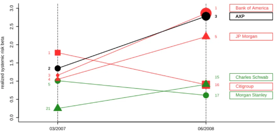
0.0 0.5 1.0 1.5 2.0 2.5 3.0 03/2007 06/2008 realiz ed systemic r isk beta 3 1 Bank of America ● 2 3 AXP ● 1 16 Citigroup 5 17 Morgan Stanley ● ● 4 5 JP Morgan 2 3 AXP ● 21 15 Charles Schwab
Figure 2: Systemic importance of five exemplary firms in the U.S. financial system at two time points before and at the height of the financial crisis, 2008. Systemic relevance is determined by the statistical significance and positivity of ”systemic risk betas” quantifying the marginal increase of the VaR of the system given an increase in a bank’s VaR while controlling for the bank’s (pre-identified) risk drivers. All VaRs are computed at the 5% level and are by definition positive. We depict the degree of systemic relevance by the size of respective “realized” versions of the systemic risk beta corresponding to the product of a risk beta and the corresponding VaR representing a company’s total effect on systemic risk. Connecting lines are added to graphically highlight changes between the two time points but do not mark real evolutions. The size of the elements in the graph reflects the size of the VaR of the respective company at each of the two time points.
We use the following scale: the element isktimes the standard size withk= 1forV aR≤0.05,
k = 1.5 forV aR ∈ (0.05,0.1], k = 2 forV aR ∈ (0.1,0.15], k = 3for V aR ∈ (0.2,0.25]
andk= 5.5forV aR ∈(0.65,0.7]. Attached numbers inside the figure mark the position of the
respective company in an overall ranking of the 57 largest U.S. financial companies for each of the two time points.
Our empirical results reveal a high degree of tail risk interconnectedness among U.S. fi-nancial institutions. In particular, we find that these network risk interconnection effects are the dominant risk drivers in individual risk. The detected channels of potential risk spillovers can to a large part be attributed to direct credit or liquidity exposures, but in some cases especially for mutual effects, they might also result from common, e.g., sector or business model specific factors, not covered by the fundamental firm specific controls in the model. In any case, these links contain fundamental information for supervision authorities but also for company risk managers. Based on the topology of the systemic
risk network, we can categorize firms into three broad groups according to their type and extent of connectedness with other companies: main risk transmitters, risk recipients and companies which both receive and transmit tail risk. From a supervisory point of view, the second group of pure risk recipients has the least systemic impact. Monitoring their condition, however, might still convey important accumulated information on potentially hidden problems in those companies which act as their risk drivers. In any case, the inter-nal risk management of these companies should account for the possible threat induced by the large degree of dependence on others. The highest attention of supervision au-thorities should be attracted by firms which mainly appear as risk drivers or are highly interconnected risk transmitters in the system. These are particularly firms in the center of the network which appear as “too interconnected to fail”, but also large risk producers at the boundary which are linked to only a few but heavily connected risk transmitters.
While the systemic risk network yields qualitative information on risk channels and roles of companies within the financial system, estimates of systemic risk betas allow to
quantifythe resulting individual systemic relevance and thus complement the full picture. Ranking companies based on (realized) systemic risk betas shows that large depositories are particularly risky. After controlling for all relevant network effects, they have the overall strongest impact on systemic risk and should be regulated accordingly. Confirm-ing general intuition, time evolutions of (realized) systemic risk betas indicate that most companies’ systemic risk contribution sharply increases during the 2007/08 financial cri-sis. These effects are particularly pronounced for firms, which indeed got into financial distress during the crisis and are (ex post) identified as being clearly systemically risky by our approach. Figure 2 exemplarily illustrates the evolutions of their marginal systemic contributions – as reflected by systemic risk betas – as well as their exposure to idiosyn-cratic tail risk – as quantified by their VaR. A detailed pre-crisis case study confirms the validity of our methodology since firms such as, e.g., Lehman Brothers are ex-ante iden-tified as being highly systemically relevant. It is well-known that their subsequent failure has indeed had a huge impact on the stability of the entire financial system. Likewise, the extensive bail-outs of American International Group (AIG), Freddie Mac and Fannie Mae
can be justified given their high systemic risk betas and high interconnectedness by the end of 2007.
The remainder of the paper is structured as follows. Section 2 describes the paper’s link to related literature and presents the underlying data. In Section 3, we present the model and estimation procedure for individual companies’ VaRs which are the basis for determining the systemic tail-risk network structure. The realized systemic risk beta is formally introduced in Section 4 and is identified for each firm in an individually tailored parsimonious partial equilibrium setting. The section also contains the corresponding estimation procedure and valid inference for a two-step quantile regression setting. Em-pirical results are presented in form of systemic risk rankings. In Section 5, we robustify and validate our model and results. In particular, in a case study using only pre-crisis data, we illustrate that the realized systemic risk beta works well in predicting the distress and systemic relevance of five large financial institutions that were affected by the financial crisis. Section 6 concludes.
2. Literature and data
2.1. Relation to the recent empirical literature
Our paper relates to several strands of recent empirical literature on systemic risk con-tributions. Building on VaR, Adrian and Brunnermeier (2011) were the first to model systemic risk contributions based on balance sheet characteristics. Their systemic impact measure, ∆CoV aR, builds on deviations of a firm’s CoVaR from a respective median benchmark. While CoVaR also aims at measuring the impact of a firm’s individual risk on the system VaR, there are, however, substantial conceptional differences to our real-ized systemic risk beta: The latter is the direct marginal effect of the individual VaR on the VaR of the system, while for CoVaR, the respective marginal effect is determined from the return and only evaluated at the VaR. As returns are in(1−q)% of the time
below its VaR(q)6, the corresponding estimated coefficient of marginal systemic impor-tance of CoVaR is generally larger and tends to systematically overrate firms with lower average returns for identical risk levels in contrast to the systemic risk beta. Furthermore, CoVaR can by definition only vary over time through the channel of individual VaRs which can, however, due to multicollinearity effects, solely be modeled as functions of macroeconomic market variables. Consequently, changes in a firm’s systemic relevance in CoVaR ultimately only result from variations in underlying macroeconomic indicators. Thus, particularly variations in a firm’s leverage or maturity mismatch as well as in its interdependence with other institutions have no direct effect. Instead, we account for net-work interconnections in the individual VaR and in its effect on the system. In addition, we identify network spillovers as crucial elements for measuring individual risk and for unbiased estimation of systemic relevance. This is illustrated in a robustness study in Subsection 3.3.1. Moreover, our realized systemic risk beta also captures variations in firms’ marginal systemic importance driven by changes in firm-specific characteristics.
Our work also complements papers measuring a company’s systemic relevance in terms of the size of potential bail-out costs, such as Acharya, Pedersen, Philippon, and Richardson (2010), Brownlees and Engle (2012) and Acharya, Engle, and Richardson (2012). Such approaches cannot detect spillover effects driven by the topology of the risk network and might tend to under-estimate the systemic importance of very intercon-nected companies. Moreover, while Brownlees and Engle (2012) study the situation of an individual firm given distress of the system, we investigate the reverse relation and measure the effect on the system given an individual firm is in financial trouble. Taking complementary perspectives, both approaches measure different dimensions of systemic risk. However, as our model is based on economic state variables and loss exceedances, it by construction automatically adjusts and prevails in distress scenarios under shocks in externalities. This is a clear advantage compared to pure time series approaches (cp. e.g., White, Kim, and Manganelli, 2010, and Brownlees and Engle, 2010) and empirically results in realized systemic risk betas indicating the raise in systemic relevance of some
companies earlier than in competing settings. We illustrate these effects in the validity case study in Section 5.2.
Furthermore, our work also complements and augments research of Billio, Getman-sky, Lo, and Pelizzon (2012) who present a collection of different systemic risk measures. These approaches mainly build on regressions in (conditional) means of returns. How-ever, assessing and predicting systemic risk and firm-specific risk requires regression ap-proaches in the (left) tails of asset return distributions, rather than in the center. Thus we quantify extreme tail situations of financial distress, which is in clear contrast to a cor-relation type analysis as in Billio, Getmansky, Lo, and Pelizzon (2012). Moreover, their determination of causality and resulting network links is entirely based on pairwise re-lations. This approach produces misleading results in a high-dimensional interconnected system as it is impossible to identify whether one firm drives another or if they are both driven by a third company. Instead, our approach yields consistent results for a mul-tivariate tail-risk network, while satisfying the Granger-causality argument in quantiles through optimal backtest performance in overall fit. Our results are also complementary to network analysis focusing on volatility spillovers in vector autoregressive systems such as in Diebold and Yilmaz (2012) and Diebold and Yilmaz (2013).
Finally, we complement macroeconomic approaches which have a more aggregated view as, e.g., the literature on systemic risk indicators (e.g., Segoviano and Goodhart, 2009, Giesecke and Kim, 2011) or papers on early warning signals (e.g., Schwaab, Koop-man, and Lucas, 2011, and KoopKoop-man, Lucas, and Schwaab, 2011).
2.2. Data
Our analysis focuses on publicly traded U.S. financial institutions. The list of included companies in Table 1 (see Appendix B) comprises depositories, broker dealers, insurance companies and Others.7 To assess a firm’s systemic relevance, we use publicly acces-7Companies are classified into these groups according to their two-digit SIC codes, following the
sible market and balance sheet data. In particular, the forward-looking nature and real-time availability of equity market data serves well to provide an immediate, actionable and transparent measure of systemic risk. The advantage of timeliness will even pre-vail if new financial regulation might force institutions to reveal information on mutual credit and liquidity linkages and leverage to supervisory authorities. At the moment, data on connections between firms’ assets and obligations is largely proprietary and far from comprehensive even for supervisors.
Daily equity prices are obtained from Datastream and are converted to weekly log returns. To account for the general state of the economy, we use weekly observations of seven lagged macroeconomic variables,Mt−1, as suggested and used by Adrian and
Brunnermeier (2011) (abbreviations as used in the remainder of the paper are given in brackets): the implied volatility index, VIX, as computed by the Chicago Board Options Exchange (vix), a short term ”liquidity spread”, computed as the difference of the 3-month collateral repo rate (available on Bloomberg) and the 3-3-month Treasury bill rate from the Federal Reserve Bank of New York (repo), the change in the 3-month Treasury bill rate (yield3m) and the change in the slope of the yield curve, corresponding to the spread between the 10-year and 3-month Treasury bill rate (term). Moreover, we utilize the change in the credit spread between BAA rated bonds and the Treasury bill rate (both at 10 year maturity) (credit), the weekly equity market return from CRSP (marketret) and the one-year cumulative real estate sector return, computed as the value-weighted average of real estate companies available in the CRSP data base (housing).8
Moreover, to capture characteristics of individual institutions predicting a bank’s propen-sity to become financially distressed,Cit−1, we follow Adrian and Brunnermeier (2011) and use (i) leverage, calculated as the value of total assets divided by total equity (in book values) (LEV), (ii) maturity mismatch, measuring short-term refinancing risk, calculated as short term debt net of cash divided by the total liabilities (MMM), (iii) the
market-to-8We found that this set of aggregate financial market variables provides sufficient explanatory power
which cannot be augmented by additional controls such as, e.g., Fama-French type factors (see Subsection 3.3.1 for details).
book value, defined as the ratio of the market value to the book value of total equity (BM), (iv) market capitalization, defined by the logarithm of market valued total assets (SIZE) and (v) the equity return volatility, computed from daily equity return data (VOL). The system return is chosen as the return on the financial sector index provided by Datastream. It is computed as the value-weighted average of prices of 190 U.S. financial institutions.9 As balance sheets are available only on a quarterly basis, we interpolate the quar-terly data to a daily level using cubic splines, and then aggregate them back to calendar weeks.10 We focus on 57 financial institutions existing through the period from beginning of 2000 to end of 2008, resulting into 467 weekly observations on individual returns. This excludes companies which defaulted during the financial crisis, but which are addressed separately in a shorter sample case study. Thus in order to validate and robustify our ap-proach, we re-estimate the model over a sub-period ending before the financial crisis and including, among others, the investment banks Lehman Brothers and Merrill Lynch that were massively affected by the crisis.
3. A tail risk network
3.1. Determining drivers of firm-specific tail risk
We measure the tail risk of a company with asset returnXi
t at time t as its conditional
Value-at-Risk (VaR),V aRiq,t, given a set of company-specific tail risk driversW(ti)
Pr(−Xti ≥V aRiq,t|W(ti)) = Pr(Xti ≤Qiq,t|W(ti)) = q (1)
9See Adrian and Brunnermeier (2011), Appendix C, who explicitly show that this induces no inherent
endogeneity in the model.
10For in-sample estimation this interpolation step captures changes in balance sheet characteristics in a
smoother way than the use of plain data. For forecasting purposes, however, interpolation is not possible. See Hautsch, Schaumburg, and Schienle (2013) for details.
with V aRi
q,t = V aRiq,t(W
(i)
t ) = −Qiq,t denoting the (negative) conditional q-quantile
of Xi
t.11 The relevant i-specific tail risk drivers are determined out of a large set of
potential regressorsWt containing lagged macroeconomic state variablesMt−1, lagged
firm-specific characteristicsCit−1, thei-specific lagged return Xi
t−1, and influences of all
other companies apart fromi, E−ti = (Etj)j6=i. We capture these intra-system influences
via contemporaneous loss exceedances, where the loss exceedance of a firmj is defined as Etj = Xtj1(Xtj ≤ Qˆj0.1) and Qˆ0.1 is the unconditional 10% sample quantile of Xj.
Hence, companyj only affects the VaR of companyiif the former is under pressure. We model the conditional VaR of firmiat time pointt= 1, . . . , T as a linear function of thei-specific tail risk driversW(ti),
V aRiq =W(i)0ξiq . (2)
This could be estimated from a corresponding linear model in the respective return quan-tile
Xti =−W(ti)0ξiq+εit, with Qq(εit|W
(i)
t ) = 0 (3)
if we knew thei-relevant risk drivers W(i) selected out ofW. Then, estimatesξbi
q of ξ
i q
could be obtained according to standard linear quantile regression (Koenker and Bassett, 1978) by minimizing 1 T T X t=1 ρq Xti+W(ti)0ξiq (4)
with loss functionρq(u) =u(q−I(u < 0)), where the indicatorI(·)is 1 foru < 0and
zero otherwise, and
[
V aRiq,t =W(ti)0bξ
i
q . (5)
However, the relevant risk driversW(i) for firm i are unknown and must be determined from W in advance. This model selection should not be imposed but should be
data-11Defining VaR as thenegativep-quantile ensures that the Value-at-Risk is positive and is interpreted as
driven. Appropriate econometric techniques are not straightforward in the given setting as tests on the individual significance of single variables do not account for the (possibly high) collinearity between the covariates. Moreover, sequences of joint significance tests have too many possible variations to be easily checked in case of more than 60 variables. We choose therelevantcovariates in a data-driven way by employing a statistical shrink-age technique known as the least absolute shrinkshrink-age and selection operator (LASSO). LASSO methods are standard for high-dimensional conditional mean regression prob-lems (see Tibshirani, 1996), and have recently been adapted to quantile regression by Belloni and Chernozhukov (2011). Accordingly, we run anl1-penalized quantile
regres-sion and calculate for a fixed individual penalty parameterλi,
e ξiq =argminξi 1 T T X t=1 ρq Xti+W 0 tξ i +λi p q(1−q) T K X k=1 ˆ σk|ξki|, (6)
with the set of potentially relevant regressors Wt = (Wt,k)Kk=1, which are demeaned,
componentwise variation σˆ2
k =
1
T
PT
t=1(Wt,k)2 and the loss functionρq as in (4). The
key idea is to select relevant regressors according to the absolute value of their respec-tive estimated marginal effects (scaled by the regressor’s variation) in the penalized VaR regression (6). Regressors are eliminated if their shrunken coefficients are sufficiently close to zero. Here, all firms in W with absolute marginal effects |eξ
i
| below a thresh-oldτ = 0.0001are excluded keeping only theK(i)remaining relevant regressorsW(i). Hence, LASSO de-selects those regressors contributing only little variation. Due to the additional penalty term in (6), all coefficientseξ
i
qare generally downward biased in finite
samples. Therefore, we re-estimate the unrestricted model (4) only with the selected rele-vant regressorsW(i)yielding the final estimatesξbi
q. This post-LASSO step produces finite
sample estimates of coefficients ξiq which are superior to the original LASSO estimates or plain quantile regression results without penalization suffering from overidentification problems (see the original paper by Belloni and Chernozhukov (2011) for the consistency proof of the post LASSO step).
The selection of relevant risk drivers via LASSO crucially depends on the choice of the company-specific penalty parameterλi. The largerλi is chosen, the more regressors are eliminated. Conversely, in case of λi = 0, we are back in the standard quantile
regression setting (4) without any de-selection. For each institution, we determine the appropriate penalty level λi in a completely data-driven way such that it dominates a respective measure of noise in the sample criterion function. In particular, we use the supremum norm of a rescaled gradient of the sample criterion function evaluated at the true parameter value as in Belloni and Chernozhukov (2011)12. In this sense, number and elements of the set of relevant risk drivers are determined only from the data without any restrictive pre-assumptions. For further details on the empirical procedure we refer to Appendix A.2.
Evaluating the goodness of fit of conditional VaR model specifications should take into account how well the model captures the specific percentile of the return distribution but also how well the model predicts size and frequency of losses. The latter issue cannot be captured, for instance, by quantile-based modifications of the conventional R2. We
therefore consider a VaR specification as inadequate if it either fails producing the correct empirical level of VaR exceedances but also if the sequence of exceedances isnot inde-pendently and identically distributed over the considered time period. This ensures that VaR violations today do not contain information about VaR violations in the future and both occur according to the same distribution. The respective formal test uses a likelihood ratio (LR) version of the dynamic quantile (DQ) test developed in Engle and Manganelli (2004) and described in detail in Appendix A.3. Berkowitz, Christoffersen, and Pelletier (2011) show that this likelihood ratio (LR) test has superior size and power properties compared to competing conditional VaR backtesting methods which dominate plain un-conditional level tests (as e.g. Kupiec (1995)).
We estimate VaR specifications withq = 0.05for all companies employing the LASSO selection procedure described above.13 Exemplary V aRi (post-)LASSO regression
re-12See Appendix A.2 Step 1 for the scaling and the exact formula.
sults for firms in the four industrial sectors depositories, insurances, brokers and others are provided in Table 2. It turns out that the main relevant drivers of company-specific VaRs are loss exceedances of other firms. In their presence, macroeconomic variables and firm-specific characteristics often do not have any statistically significant influence and are not selected by the LASSO procedure. In Table 2, only for Torchmark (TMK) and Regions Financial (RF) regressors other than cross-firm links are selected. In contrast, VaR specifications of Goldman Sachs (GS), Morgan Stanley (MS), JP Morgan (JPM) and AIG exclusively contain loss exceedances from other firms. The general importance of cross-firm effects as main drivers of individual tail risks is confirmed by joint significance test of the individually selected loss exceedancesE−ti and by the superior VaR forecast performance. Please see the robustness Subsection 3.3 for details.
With our procedure we statistically detect “relevant” directional risk connections in the financial sector. Certainly, there might be several types of economic causes for a link between two companies which can, however, empirically not be further identified from publicly disclosed market data.14 By including firm-specific characteristics and macroe-conomic state variables in our model, we do prevent, however, that determined risk con-nections result from common economic conditions or common risk factors. Hence, we rule out that tail dependencies are driven, for instance, by periods of high volatility, flatten-ing of yield curves or fallflatten-ing overall credit quality. Accordflatten-ingly, risk links are attributed to remaining factors which are most likely direct or indirect credit or liquidity exposures or, in some cases, business model commonalities or sector specific risk factors. In this sense, connections between close competitors, such as Goldman Sachs and Morgan Stan-ley and the influence of mortgage company Freddie Mac (FRE) on AIG both confirm market evidence.
14Note that a valid empirical classification into different types of linkages would require comprehensive
data on direct and indirect credit and liquidity exposures of firms. Such information, however, is in large part not publicly available.
3.2. Network model and structure
We constitute a tail risk network of the system from individually selected loss exceedances reflecting cross-firm dependencies.15 Taking all firms as nodes in such a network, there is an influence of firm j on firm i, if Ej is LASSO-selected in (6) as a relevant risk
externality of firmi inV aRiq. In particular, ifEj is part ofW(i) as its k-th component, then the corresponding coefficientξi
q,k in ξ
i
q marks the risk impact of firmj on firmiin
the network. If Ej is not selected as relevant risk driver of firm i, there is no network
arrow from firmj to firmi.
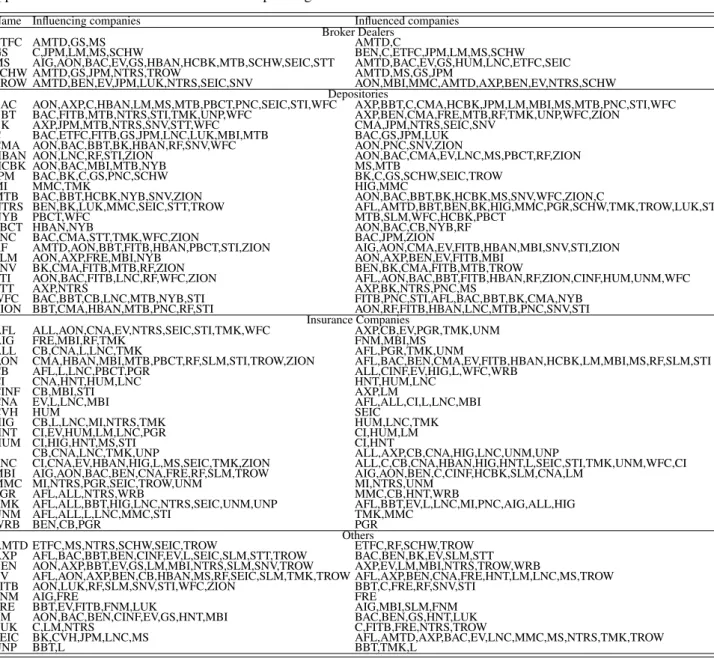
As in the previous subsection, we use VaR specifications withq = 0.05. An overview of the identified tail risk connections between all companies is provided in Table 3 re-porting which company’s loss exceedance affects which others’ VaR and vice versa. We observe that the number of risk connections substantially varies over the cross-section of companies. While some firms such as, e.g. , Morgan Stanley, Bank of America (BAC), American Express (AXP) as well as Bank of New York Mellon (BK), are strongly inter-connected with many other companies, there are institutions, such as Fannie Mae (FNM), AIG (AIG) and a couple of further insurances revealing significantly less cross-firm de-pendencies. In order to effectively illustrate identified risk connections and directions, we graphically depict the resulting network of companies in Figure 6. The layout and allo-cation of the network is chosen such that the sum of cross-firm distances is minimized. Consequently, the most connected firms are located in the center of the network while the less involved companies are placed on its boundary.
The resulting network topology reveals different roles of companies within the finan-cial network. We distinguish between three major categories: The first group contains companies with only few incoming arrows but numerous outgoing ones and thus mainly act as risk drivers within the system. These are institutions whose potential failure might affect many others but, conversely, which are themselves relatively unaffected by the
dis-15In the Bayesian network literature, networks which build on direct one-step influences constitute a
so-called Markov blanket assumed to contain all relevant information for predicting the node’s role in the network (see Friedman, Geiger, and Goldszmidt, 1997).
tress of other firms. They should be the focus of close monitoring by supervisory authori-ties as a failure of such a company might induce substantial systemic risk through multiple channels into the financial network. Our results show that only few firms belong to this category. Examples are State Street Corporation (STT), one of the top ten U.S. banks, Leucadia National Corporation (LUK), a holding company which is, among others, en-gaged in banking, lending and real estate, and SEI Investments Company (SEIC), a finan-cial services firm providing products and service in asset and investment management. Financial distress of these banks obviously has wide-spread consequences. For instance, State Street influences the financial services companies American Express and Northern Trust (NTRS), the Bank of New York Mellon and Morgan Stanley. Leucadia affects Cit-igroup (C), one of the biggest banks in the U.S., and Freddie Mac, one of the two largest U.S. mortgage companies. Finally, SEI Investments has links to various big institutions, such as Bank of America, American Express, Morgan Stanley and the online broker TD Ameritrade (AMTD).
The second group contains companies which mainly are risk takers within the system. These companies are not necessarily systemically risky but might severely suffer from distress of others and should account for such spillovers in their internal risk manage-ment. According to Table 3 and Figure 6 these firms are primarily insurance companies. Examples are Cincinnati Financial Corporation (CINF), a company for property and casu-alty insurance, Humana Incorporation (HUM) managing health insurances or Progressive Corporation Ohio (PGR) providing automobile insurance and other property-casualty in-surances.
The third group is the largest category within the network. It consists of companies which serve as both risk recipients and risk transmitters amplifying tail risk spillovers by further disseminating risk into new channels. Due to their role as risk distributors, such companies are key systemic players and should be supervised accordingly.
We further distinguish between strongly and less connected firms. The focus of super-vision authorities should be on a close monitoring of the first subgroup. Examples are
Goldman Sachs, Citigroup, Morgan Stanley, AON Corporation (AON), Bank of America, American Express, Freddie Mac as well as the insurance company MBIA (MBI), among others. Bank of America and Citigroup are among the five largest banks in the U.S. and reveal strong connections to various other big institutions, such as Morgan Stanley, JP Morgan, Goldman Sachs, American Express, Regions Financial and AIG. Details on the specific role of Citigroup and Morgan Stanley within the system are highlighted in Figure 7. Morgan Stanley, with strong links to many companies, such as Goldman Sachs, Bank of America, the savings bank Hudson City Bancorporation (HCBK), and the insurance company AON, are examples for deeply connected firms located in the center of the net-work. Likewise, Freddie Mac is strongly involved and was particularly affected by the 2008 credit crunch in the mortgage sector. Accordingly, also MBIA realized severe losses during the financial crisis due to investments in mortgage backed securities.
The second subgroup might be technically easier to monitor with companies revealing risk connections with only very few other firms. Still, a close and detailed supervision is not less important than for the first subgroup. Examples are Fannie Mae and AIG. Fannie Mae reveals significant bilateral risk connections to its main competitor Freddie Mac. AIG holds significant positions in mortgage backed securities and as a consequence is closely connected to both Fannie Mae and Freddie Mac. Probably due to the same reason, we also observe bilateral tail risk dependencies between AIG and MBIA. Even though their number of relevant risk connections within the network is limited, such firms can still have a crucial overall impact on the system. In case of the 2008 financial crisis, the dependence between Freddie Mac and Fannie Mae as well as their interaction with AIG had severe systemic consequences.
Figure 8 indicates that it is not sufficient to focus on sector-specific subnetworks only. Indeed interconnectedness of institutions occurs to a large proportionbetweenindustrial sectors. In these circle layout network graphs, companies are grouped according to in-dustries with risk outflows for each group being highlighted. We observe that tail risks of depositories, insurances and others are relatively equally distributed among all other industry groups. Depositories are most strongly connected and also reveal the strongest
tail risk links among each other. This is in contrast to the other industries where cross-firm connectionswithina group are less strong. Moreover, in contrast to other industry cate-gories, the risk outflow of broker dealers is clearly more concentrated. They particularly affect big banks such as Bank of America and Citigroup as well as financial service com-panies such as American Express or SEI. Only very few direct connections to insurance companies are revealed.
3.3. Robustness
3.3.1. Network model validity
Given our data set, it is sensible to base our tail-risk networks on VaR levels ofq = 5%. More extreme probabilities are theoretically feasible but require a larger amount of ob-servations for sufficient statistical precision. We have also experimented with different thresholds in the loss exceedances but found that for the present data, the 10% quantile optimally balances the trade-off between requiring sufficient number of nonzero observa-tions inE−ti and a sufficient number of extreme losses.
The significance of network effects in the individual VaR specifications can be formally tested via a joint significance test of the individually selected loss exceedancesE−tiin the respective quantile regression (2). We have performed this analysis based on a quantile regression version of the F-test for joint linear hypotheses developed by Koenker and Bassett (1982). Our results show that the selected tail risk spillovers are highly significant in all but very few cases. See Table 3 for an overview of all cross-effects. The detailed test results are available upon request.
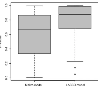
The importance of including other companies’ loss exceedances as potential risk drivers for a companyiis also illustrated by a simple comparison of the (in-sample) forecast per-formance of our LASSO-selected VaR specifications to corresponding models forV aRi
only using macroeconomic variables as in Adrian and Brunnermeier (2011). According to the employed backtests, specifications allowing for cross-firm dependencies reveal a
0.0 0.2 0.4 0.6 0.8 1.0
Makro model LASSO model
P−V
alues
Figure 3: Boxplots of backtestingp-values indicating the in-sample model fit (i.e., test-ing the null hypothesis of formal statistical adequacy) of VaR specifications includtest-ing macroeconomic regressors only (left) and VaR specifications resulting from the LASSO selection procedure (6) (right).
strong predictive ability and are significantly superior to more simplistic models including macroeconomic regressors only (and ignoring network linkages). Figure 3 illustrates the distributions of the backtestingp-values implied by both models. Hence, inter-company linkages add crucial explanatory power in VaR specifications.
Network effects also remain important when altering the set of economic state vari-ablesMby typical equity risk premium factors. In particular, we re-estimated the model including four lagged weekly asset pricing factors, including the three Fama-French fac-tors and the momentum factor according to Carhart (1997).16 However, in the presence of network exceedances, these factors have been de-selected in all cases by the LASSO method and thus have had no additional relevance for our model specification. This indi-cates that the tails of asset returns are driven by other sources than the equity risk premium (associated with return’s conditional mean).
Our results show that the major information about cross-company dependencies in tail risks is primarily contained incontemporaneous loss exceedances E−ti. In contrast, alternative VaR specifications utilizing contemporaneous returnsXt−j or lagged loss ex-ceedancesE−t−1i imply significantly inferior backtest performances with the regressors
be-16The data are downloaded from the website of Kenneth French on
ing mostly not significant in joint F-tests.17 Moreover, linking VaR forecasts and thus predictions of hypothetical losses to already realized loss exceedances allows measur-ing mutual dependencies between companies without requirmeasur-ing a simultaneous system of equations in conditional quantiles. In particular, observed bi-directional relationships between conditional quantiles and realized loss exceedances of different firms (e.g., be-tween Goldman Sachs and Morgan Stanley) do not reflect simultaneities as feedbacks are not contemporaneous: For instance, a highly negative (realized) return of companyj in-creases the conditional loss quantile and therefore inin-creases the VaR of firmi. However, a higher conditional VaR ofidoes not necessarily directly increase the absolute realized loss return ofibut just makes it more likely. Avoiding an explicit treatment of simultane-ities in quantiles while still addressing network dependencies is an important advantage of our approach.18
3.3.2. Accuracy of the LASSO selection step
The firm-specific LASSO penalty parameterλiis a crucial parameter in our approach as it determines the denseness of the risk network, and also influences the outcomes from the second stage systemic risk measure in Section 4. It is chosen in a completely data-driven procedure, such that a backtest criterion is optimized (see Sections 3.1 and A.2). To vali-date this model selection step and to assess whether the procedure prevents overfitting, we analyze the consequences of increasing the LASSO penalty parameter. Note that higher values ofλilead to selections of smaller models. If our procedure had a tendency to overfit the tails, the overall goodness of fit would increase for higher values ofλi. This
possi-bility is checked by increasing all penalty parameters by 10% and 20%, and analyzing two different measures of fit for the resulting models.19 Firstly, according to our backtest
17The corresponding results are available upon request and omitted here for sake of brevity.
18Econometrically it is an open question how to handle such a system in conditional quantiles in general.
In contrast to relations in (conditional) means, it is unclear how marginalq-quantiles constitute the respec-tive quantile in the joint distribution under appropriate independence assumptions. Only in lags, restricted to very small dimensions and under strong assumptions, solutions have been obtained via CaViAR type structures (see White, Kim, and Manganelli (2010)).
19It turns out that increasing the penalties beyond 20% is not advisable as for a number of VaRs, no
criterion, the overall goodness of fit deteriorates substantially, which is demonstrated by three boxplots and exemplary illustrations of individualp-values shown in Figure 12. It turns out that for higher values ofλi, thep-values decrease and thus the statistical support
for the null hypothesis of a good model fit declines. Likewise, joint significance tests do not support the exclusion of additional regressors due to higher penalties. In particular, it turns out that the additionally de-selected regressors are mostly significant (jointly with the selected ones). This finding is further robustified by a second goodness of fit measure corresponding to a Bayesian Information Criterion (BIC) for quantile models proposed by Lee, Noh, and Park (2013). As shown by Figure 12, the BIC is increasing and thus indicates a less favorable model if the penalty parameter is increased. These evaluations support our choice of penalization and indicate that there is no evidence for a tendency of overfitting the tails.
3.3.3. Network characteristics
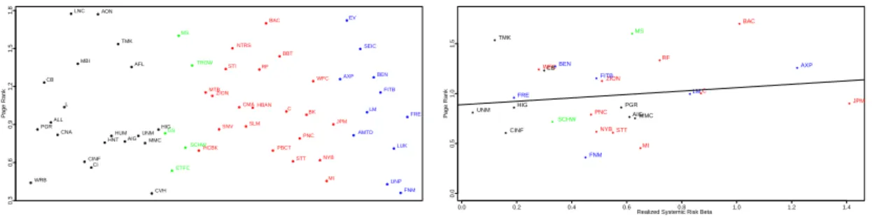
Besides graphical illustration and inflow-outflow categorizations, standard network char-acteristics can provide a more comprehensive picture of the interconnectedness and the role of each network node in the system. In Figure 4, we depict firms’ pagerank co-efficient (see Brin and Page (1998)) which does not plainly count links but empirically weights their importance in an iterative scheme.20 Confirming the visual impression based on Figure 6, the most connected firms are Lincoln National Corporation, AON, Bank of America, TD Ameritrade and Morgan Stanley. The graph confirms our finding above that depositories tend to be slightly stronger involved than other industry groups. Particularly insurances reflect a separation into a group of highly connected firms, such as Lincoln National Corp., AON and MBI, and a group of companies being less connected, such as AIG, Humana Incorp. , Unum Group (UNM) and Cincinnati Financial Corp.
20The key idea is to assign a weight to each node (i.e., a company in our context) which is increasing
with the number of connections to others and the relative importance thereof. The more connected a firm is, the higher its importance and thus the higher the importance of its neighbor. The computation of the pagerank coefficient can be understood as an eigenvalue problem which can be solved iteratively. For more details, see Berkhin (2005).
● ● ● ● ● ● ● ● ● ● ● ● ● ● ● ● ● ● ● ● ● ● ● ● ● ● ● ● ● ● ● ● ● ● ● ● ● ● ● ● ● ● ● ● ● ● ● ● ● ● ● ● ● ● ● ● ● 0.3 0.6 0.9 1.2 1.5 1.8 P age Rank WRB PGR CB ALL CNA L LNC MBI CINF CI AON HNT HUM TMK AIG AFL UNM MMC CVH HIGGS ETFC MS SCHW TROW HCBK MTB ZION SNV STI NTRS CMA SLM HBAN RF BAC PBCT BBT C STT PNC BK WFC NYB MI JPM AXP EV AMTD SEIC LM BEN FITB UNP LUK FNM FRE ● ● ● ● ● ● ● ● ● ● ● ● ● ● ● ● ● ● ● ● ● ● ● ● ● ● 0.0 0.5 1.0 1.5 0.0 0.2 0.4 0.6 0.8 1.0 1.2 1.4 P age Rank
5HDOized 6\VWHPLF5LVNBeta PGR CB CINF TMK AIG UNM MMC HIG MS SCHW ZION RF BAC C STT PNC NYB MI JPM WFC AXP LM BEN FITB FNM FRE
Figure 4: The left figure displays pagerank coefficients based on the estimated tail risk network computed as in Berkhin (2005) with ordering of institutions according to sectors. On the right, pagerank coefficients are plotted versus realized systemic risk contributions measured as average realized systemic risk betas (8) for all companies which are classified as systemically relevant for the years 2000-2008 according to Subsection 4.3. The regression line shows only a small correlation between the pagerank coefficent and the realized systemic risk beta, supported by the
respectiveR2of 0.0265 of the regression. Colors and acronyms are as in Figure 1.
Note that pagerank coefficients such as other network metrics can only assess the local impact and centrality of firms in the network containing relevant but not all information for judging overall systemic relevance. Therefore, a risk network does not allow to fully quantitatively assess the systemic relevance of a financial institution. Nevertheless, the degree of firms’ interconnectedness and the specific topology of the network or corre-sponding sub-networks allows identifying possible risk channels in the system. These interlinkages are central but not comprehensive for macroprudential regulation reflecting the particular role of a firm as risk recipient, transmitter or distributor of tail risk. To ex-plicitlyquantifya firm’s marginal systemic relevance, we propose the concept of systemic risk betas presented in the following section.
4. Quantifying systemic risk contributions
4.1. Measuring and estimating systemic risk betas
Besides valuable information on financial network structures, the focus of supervision authorities is on an accurate but parsimonious measure of an institution’s systemic impact. We quantify the latter as the effect of a marginal change in the tail risk of firmi on the
tail risk of the system given the underlying network structure of the financial system. As for firm’s tail risk in equation (1), system tail risk is measured as the respective Value-at-RiskV aRs
p,tof the system returnXtsconditional onV aRiq,tand other controls. Then, we
define thesystemic risk betaas the marginal effect of firmi’s tail risk on the system tail risk given by ∂V aRs p,t(V (i) t , V aRiq,t) ∂V aRi q,t =βp,qs|i, (7)
whereVt(i)are firm-specific control variables.21 It can be interpreted in analogy to an in-verse asset pricing relationship in quantiles, where banki’sq-th return quantile drives the p-th quantile of the system given network-specific effects and firm-specific and macroe-conomic state variables. We classify the systemic relevance of institutions according to their statistical significance ofβp,qs|i at a given level and the size of their total effect
¯
βp,qs|i :=βp,qs|iV aRit, (8)
which we denote as realized systemic risk contribution since it is computed based on market realizations. In contrast to the marginal systemic risk beta, the realized version captures the full partial effect of a tail risk increase of bankionV aRst and is thus cross-sectionally comparable across banks.
Focusing on an unbiased estimate of a firm’s marginal effect, we employ for each company a tailored i-specific model for V aRs in (7) which allows correctly evaluating
the desired effectβp,qs|i. In particular, in each of this partial system VaR models, it is
nec-essary but sufficient to control for firms which are relevant i-specific risk drivers in the network inV aRs. Conversely, variables unrelated toV aRido not affect firmi’s systemic
risk contribution and can be omitted in a respective parsimonious model.22 In this way, we circumvent involved theoretical specification issues and econometric feasibility and
preci-21Note that we only study theimmediateeffect of an exogenous risk shock in companyifor the system.
We do not infer about further steps which should then also account for converse effects of increases of system risk causing firm-specific risk to raise. This would require a further involved dynamic modeling step which is beyond the scope of this analysis.
22See Angrist, Chernozhukov, and Fernández-Val (2006) for a simple Frisch-Waugh-type argument in
sion problems of alternative comprehensive structural general equilibrium models. Even if correctly specified, such complete models would suffer from the high dimensionality and interconnectedness of the financial system in the presence of limited data availability. See Section 5 for an empirical comparison.
Consequently, we estimate the firm-i-specificsystemic risk betaβq,ps|i based on a linear
model for the system VaR of the form
V aRp,ts =V(ti)0γps+βp,qs|iV aRiq,t, (9)
where the vector of regressors V(ti) = (1,Mt−1,VaR (−i)
q,t ) includes a constant effect,
lagged macroeconomic state variables and the VaRs of all companies which are identi-fied as risk drivers for firmivia LASSO in Section 3.
Systemic risk betas in (9) are moreover allowed to be explicitly time-varying, account-ing for periods of turbulence where not only banks’ risk exposures change but also their marginal importance for the system might vary. In particular, we model potential time-variation of βs|i through a linear model in observable factors Zi which characterize a bank’s propensity to get in financial distress. As a function of lagged characteristics, such
conditional systemic risk betas and thus corresponding systemic risk rankings are pre-dictable which is important for forward-looking monitoring and supervision of the finan-cial system. Furthermore, linearity ofβp,q,ts|i in firm-specific distress indicatorsZit−1 yields stable main effects, given the quarterly reporting frequency of these factors. The quality of generally available data limits the expected potential for improvements stemming from other functional forms or nonparametric estimates which would in any case substantially increase the statistical complexity and computational burden within the two-step model. Thus we set
βp,q,ts|i =β0s,p,q|i +Zit−10ηsp,q|i, (10)
The firm-specific time-varying systemic risk beta βp,q,ts|i can then be estimated from the (second step) quantile model (9) for V aRs
p with time variation according to (10).
The respective quantile regression becomes operational when using post-LASSO pre-estimates V aR[it and VaRd
(−i)
q,t from (6) in the respective components of V
(i)
for those regressors not directly observed in the data.23 Hence,
Xts =−β0s|,p,qi V aR[iq,t−(V aR[iq,t·Zit−1) 0 ηsp,q|i −Vd(i) 0 tγ s p+ε s t, (11) whereQp(εst|V aR[ i q,t,Vb (i) t ,Z i
t−1) = 0. Then, as in the first-step regressions in Section 3,
estimates of all components ofβp,q,ts|i are obtained via quantile regression minimizing
1 T T X t=1 ρp(Xts+V 0 tξ s) (12)
in the unknown parametersξs where Bt ≡ (V aRit, V aRit ·Z i
t−1,V
(i)
t )is the compound
vector of all regressors inV aRsp. This yields the resulting estimate of the full time-varying marginal effectβb s|i p,qin (10), b βp,q,ts|i =βb s|i 0,p,q+Z i t−1 0 d ηp,qs|i, (13)
for given valuesZit−1. Constant systemic risk betas can obviously be obtained as a special case under the restrictionηsp,q|i = 0in the estimation (12) yielding βb
s|i p,q,t = βb s|i 0,p,q = βb s|i p,q.
The realized beta (8) is estimated asbβ¯
s|i p,q,t :=βb s|i p,q,tV aR[ i t.
For valid inference, however, the fact that certain regressors are not observed but only pre-estimated has crucial consequences. In particular, the quantile regression asymptotic standard errors of usual software packages based on Koenker and Bassett (1978) are
gen-23Note that a direct one-step plug-in version of the proposed two-step estimation strategy is not feasible
and leads to an identification problem. Inserting the linear individual VaR (2) into the linear sytem VaR model (9) yields a full model for the system’s tail risk in observable characteristics. But model selection based on such a full model forV aRsin observables is infeasible since correlation effects among the huge number of regressors would produce unreliable results. Furthermore, individual parametersβs0|,p,qi andηsp,q|i
could not be identified without additional identification conditionQq(εit|W (i)
t ) = 0, implicitly bringing
erally too small not accounting for the pre-step. In contrast to mean regressions, such two-step results are non-standard in a quantile setting and are therefore provided in detail in Appendix A.1. Up to our knowledge, they are new to the literature.
4.2. Determining systemic relevance
We determine systemic relevance and potential time variation thereof via formal statistical significance tests. Though, respective quantile versions of asymptotic t- or F-tests are not valid in finite samples and simple direct bootstrap adaptations yield incorrect results for quantiles.24 Therefore, we propose to base a finite sample test for any linear hypothesis
Hofβˆp,q,ts|i on the type of test statistic statistic given by
ST = min ξs∈Ω T X t=1 ρp(Xts+B 0 tξ s )− min ξs∈ RKB T X t=1 ρp(Xts+B 0 tξ s ), (14)
with regressorsBtand correspondingKB-parameter vectorξsas in the system VaR
spec-ification (12), andΩreferring to the constrained set of parameters ofβˆp,q,ts|i underH. This test is an adaptation to the quantile setting of a method proposed by Chen, Ying, Zhang, and Zhao (2008) for median regressions. Direct operationalization of the test is com-plicated by the fact that the asymptotic distribution of 14 involves unknown terms, and by the non-smooth objective function of the quantile regression causing inconsistency of conventional resampling techniques. Therefore, following Chen, Ying, Zhang, and Zhao (2008), we provide an adjusted “wild-type” bootstrap method, which is described in detail in Appendix A.4. We generally consider effects as being significant ifp-values are below 10%.
We define a company as systemically relevant if an increase in its possible loss posi-tion, given all economic state variables andi-specific risk inflows from other companies,
24Generally, asymptotic distributions often only provide a poor approximation to the true distribution of
the (scaled) difference between the estimator and the true value if sample sizes are not sufficiently large. In case of quantile regressions, this effect is even more pronounced, since valid estimates for the asymp-totic variance have poor non-parametric rates and thus require even larger sample sizes to obtain the same precision.
induces a significantly higher potential systemic loss. This requires its systemic risk beta to be significantand nonnegative.25 The potentially time-varying degree of systemic rel-evance is then measured according to the size of its realized beta at the respective point in time. We can thus determine if a company is systemically relevant by testing for the significance of the respective systemic risk beta, which is the joint significance of all components ofβts|i. Thus, we test the hypothesis
H1:β0s|i =ηM M Ms|i =ηsSIZE|i =ηLEVs|i =ηBMs|i =ηV OLs|i = 0.
Whether marginal effects on the system are indeed time-varying in firm-specific char-acteristics can be tested by the joint hypothesis
H2:ηsM M M|i =ηSIZEs|i =ηLEVs|i =ηBMs|i =ηV OLs|i = 0.
If H2 is not rejected, we re-specify the systemic risk beta as being constant (βts|i = βs|i),
re-estimate the model without interaction variables and test the hypothesisH3:βs|i = 0.
4.3. Empirical results and robustness of systemic risk betas and risk
rankings
We estimate potentially time-varying systemic risk betas according to (12). As in the first-step estimations, we chooseq= 0.05, i.e., we model the loss which will not be exceeded with 95% probability. For notational convenience, we suppress the quantile index as we set p = q. As potential drivers of time-variation in systemic risk betas, we take all firm-specific tail risk drivers, i.e.,Zit = Cit, since size, leverage, maturity mismatch, book-to-market ratio and volatility might not only affect a bank’s VaR, but also directly
25Since we do not impose a priori non-negativity restrictions, systemic risk betas can become negative at
certain points in time. In a few cases we can directly attribute these effects to sudden time variations in one of the (interpolated) company-specific characteristicsZit−1driving systemic risk betas temporarily into the negative region. These effects might be reduced by linkingβs|i in (10) to (local) time averages ofZi
t−1.
This stabilizes systemic risk betas but at the cost of a potentially high loss of information. We see this as an alternative approach which, however, is not pursued in the given context.
determine its marginal systemic effect. As a consequence, systemic risk contributions of two companies with the same exposure to macroeconomic risk factors and financial network spillovers may still differ due to their balance sheet structures.26
We find that the majority of firms have a significant systemic risk beta, which is clas-sified as being time-varying in approximately 50% of all cases. In contrast, for approx-imately 25%of all firms, we do not find systemic risk betas which are significantly dif-ferent from zero. Table 4 reports thep-values of the respective underlying tests which are performed using the wild bootstrap procedure illustrated in Appendix A.4 based on
2,000 resamples of the test statistic.27 Table 5 lists all systemically relevant companies for the period from 2000 to 2008, ranked according to their average realized systemic risk contributionsβˆ¯s|i. The top positions of the systemically most risky companies are taken by JP Morgan, American Express, Bank of America and Citigroup. According to our network analysis above, these firms are also categorized into the group of risk amplifiers which are strongly interconnected and should thus be closely monitored.
Obtained realized systemic risk betas, however, contain information on systemic rel-evance beyond a company’s network interconnectedness. This is illustrated in Figure 4 revealing only slightly positive dependencies between pagerank coefficients and realized systemic risk betas. Thus, more connected firms tend to be systemically more risky, see e.g. , Bank of America and American Express. With anR2 of 2%in the regression, the relationship, however, is not very strong indicating that the quantification of a firm’s inter-connectedness is not sufficient to assess its systemic relevance which directly depends on firm-specific and macroeconomic conditions. The latter is captured by realized systemic risk contributions but not necessarily by pagerank coefficients.
26Note that we keep the set of regressorsM parsimonious as described in Section 2.2. According to
Subsection 3.3.1) the increase in explanatory power stemming from additional factors such as, e.g., Fama-French/Carhart factors is low in the presence of network effects and thus can be neglected.
27Because of multi-collinearity of time variation effects in firm characteristics for systemic risk betas,
the interpretation of individual coefficientsη might be misleading. Therefore, we refrain from reporting respective estimates.