Regensburger
DISKUSSIONSBEITRÄGE
zur Wirtschaftswissenschaft
University of Regensburg Working Papers in Business,
Economics and Management Information Systems
Single-Name Credit Risk, Portfolio Risk, and Credit Rationing
Lutz G. Arnold
∗Johannes Reeder
Stefanie Trepl
19.10.2010
Nr. 448
JEL Classification:
D82, E51, G21
Key Words: asymmetric information, credit rationing
∗
Single-Name Credit Risk, Portfolio Risk, and Credit Rationing
Lutz G. Arnold Johannes Reeder Stefanie Trepl University of Regensburg Department of Economics 93 040 Regensburg, Germany Phone: +49-941-943-2705 Fax: +49-941-943-1971 E-mail: lutz.arnold@wiwi.uni-r.de AbstractThis paper introduces non-diversifiable risk in the Stiglitz-Weiss adverse selection model, so that an increase in the average riskiness of the borrower pool causes higher portfolio risk. This opens up the possibility of equilibrium credit rationing. Comparative statics analysis shows that an increase in risk aversion turns a two-price equilibrium into a rationing equilibrium. A two-price equilibrium is more inefficient than a rationing equilibrium, and a usury law that rules out the higher of the two interest rates can be welfare-improving. Contrary to the common result, the equilibrium may be characterized by over-investment.
JEL classification: D82, E51, G21
1
Introduction
Models of adverse selection or moral hazard in the credit market show why lenders tend to finance investment projects which are too risky from their point of view. The reason why lenders dislike risky projects is that, when standard credit contracts are used, they generate lower expected repayment. Due to the common assumption of independence of the payoffs on different projects and the law of large numbers for large economies (Uhlig, 1996), the repayments on a well-diversified credit portfolio are safe, however (an implication that tends to irritate scholars with a background in portfolio theory): uncorrelated single-name credit risks cancel out and do not create any portfolio risk for the lender. A notable case in point is the seminal Stiglitz-Weiss (1981) (henceforth: “SW”) adverse selection model, in which an increase in the interest rate raises the average riskiness of the pool of active borrowers, but nonetheless the return on lending remains safe.
The present paper introduces non-diversifiable risk to the SW model (with two borrower types), so that an increase in the average riskiness of the borrower pool causes higher portfolio risk, which has to be borne by lenders. This has several interesting implications for equilibrium and welfare. First, it opens up the possibility of equilibrium credit rationing. As shown independently by Coco (1997) and Arnold and Riley (2009), non-monotonicity of the expected repayment lenders receive as a function of the interest rates potentially gives rise to a two-price equilibrium with market clearing at the higher rate in the SW model. There cannot be pure rationing at a single interest rate in the SW model, because it would be profitable to serve rationed risky borrowers at their maximum acceptable interest rate.1 This strategy of “picking risky borrowers” might be unattractive to risk-averse lenders when the project payoffs are correlated, since it gives rise to a highly risky credit portfolio. Thus, a profitable deviation from the strategies that lead to rationing may not exist, restoring the possibility of equilibrium credit rationing.
A two-price equilibrium entails higher average project risks and, hence, higher portfolio risk than a rationing equilibrium, at a given level of investment. This is because market clearing at the higher interest rate implies that all risky projects are financed. As a consequence, whether a two-price equilibrium or a rationing equilibrium arises depends systematically on lenders’ degree of relative risk aversion. To address this issue, we use the constant relative risk aversion (CRRA) version of the Ordinal Certainty Equivalent (OCE) utility function proposed by Selden (1978), which allows to disentangle changes in risk aversion from changes in the preference for consumption smoothing over time. We show that starting from a two-price equilibrium, a rationing equilibrium arises when
1Bester (1985, 1987), Riley (1987), Lensink and Sterken (2002), and De Meza and Webb (2006) provide alternative
(everything else equal) the degree of relative risk aversion grows sufficiently large. Thus, stronger risk aversion tends to make the emergence of a rationing equilibrium more likely.
A two-price equilibrium is, in a specific sense, more inefficient than a rationing equilibrium: consider a parameter change that leads to a switch from a two-price equilibrium to a rationing equilibrium. The level of investment is continuous in model parameters, so it changes only slightly. However, the riskiness of the pool of active borrowers deteriorates discontinuously, since all risky firms get finance in a two-price equilibrium. As a consequence, borrowers have to pay higher risk premia, so aggregate profit and total welfare jump downward. One way to avoid this inefficiency of a two-price equilibrium is to impose a usury law that prohibits interest rates above the equilibrium rate with pure rationing. Analogous results are derived by Coco (1997, Section 3) in a model with independent returns in which projects differ by both riskiness and mean return.2
Following De Meza and Webb (1987), next we address the question of whether there is too little or too much investment in equilibrium, relative to a first-best or a second-best optimum. Contrary to the common result that equilibrium is generally characterized by under-investment, we find that equilibrium over-investment may arise in a two-price equilibrium or in a rationing equilibrium, viz., when firms are endowed with a large amount of collateral and little weight is put on their expected utility in the optimum solution. Under these conditions, optimum saving is low, and may thus fall short of equilibrium investment, because households’ consumption can be satisfied by reallocating the firms’ collateral to them.3
The motivation for the analysis is the observation that returns on risky investment projects are correlated, so that someone has to bear the additional risk when firms carry out riskier investment projects. While direct evidence of correlation between individual firms’ returns on investment is hard to come by, there are numerous country studies showing that economy-wide and industry factors explain much of the variance in firm earnings (e.g., Brealey, 1971, for the U.S.), that firm-level profitability is strongly affected by aggregate demand shocks (e.g., Machin and van Reenen, 1993, for the U.K.), and that macroeconomic shocks have a profound impact on business failures (e.g., Gaffeo and Santoro, 2009, for Italy). Generally, the fact that aggregate corporate profits are strongly procyclical means that individual firms’ profits are positively correlated at business cycle frequency. These observations suggest that there is significant correlation between the returns
2See also De Meza and Webb (2006).
3This relates to variants of the SW model concerned with optimal risk sharing, such as Bester (1985, 1987) (see
also the survey in Coco, 2000). These models usually assume risk-averse borrowers and independent project risks (i.e., no risk for lenders) and highlight the welfare loss due to the use of collateral as a sorting device: since a borrower’s marginal utility is higher when his project fails, he should not put up any collateral in a first-best optimum.
on individual firms’ risky endeavors. One might object that, even so, independence would be a convenient assumption if it reduced complexity without having a major impact on the results. However, the summary of the results above shows that the introduction of non-diversifiable risk leads to much richer model implications, as different types of non-market clearing equilibria emerge depending on consumers’ risk attitudes, with interesting welfare implications.
Section 2 presents the model with CRRA preferences. In Section 3, we demonstrate that pure credit rationing can arise. Section 4 introduces OCE preferences and analyzes the impact of the degree of risk aversion on the type of equilibrium. Section 5 highlights the inefficiency of a two-price equilibrium. Section 6 addresses the question of equilibrium under-investment. Section 7 concludes.
2
Model
There are two time periods t = 1,2. There is one homogeneous (perishable) good, which can be used for consumption or investment. There is a continuum of measure M (>0) of identical risk-averse consumers, each endowed with y (> 0) units of the homogeneous good in the first period and nothing in the second period. So to consume in period 2, they have to save in period 1. The consumers’ preferences are represented by the CRRA utility function
E[u(c1, c2)] = c 1−θ 1 1−θ +δE c12−θ 1−θ , 0< δ, θ <1, (1)
where ct is period-t consumption of the homogenous good (t = 1,2). θ measures the inverse of
the intertemporal elasticity of substitution in consumptionandthe degree of relative risk aversion. The assumption that 1/θis greater than one ensures that capital supply is upward-sloping, so that the analysis is comparable to the existing literature. In the model with OCE preferences, we will maintain the assumption that the intertemporal elasticity of substitution exceeds unity but allow for arbitrary positive degrees of relative risk aversion.
There are a continuum of measure NS (>0) of safe firms and a continuum of measure NR (>0)
of risky firms, each endowed with collateral C (> 0) and the ability to turn B (> C) units of the homogeneous good invested in the first period into a random second-period output of the homogeneous good. Safe firms’ projects succeed with with probability pS and risky firms’ projects with probability pR (0 < pR < pS < 1). In case of success, they yield RS or RR, respectively. If
a project fails, the payoff is zero. The projects are equally profitable on average: pSRS = pRRR
(≡R > B¯ ). Standard debt is the only financial instrument.4 Firms’ collateral C cannot be traded
4Standard debt is the optimal mode of finance in related models, e.g., when lenders can observe whether a project
in the capital market.5 Firm owners are risk-neutral and apply for capital if the expected return on their investment (taking care of the possibility that they lose their collateral) is non-negative. There is asymmetric information: lenders are unable to observe whether a firm owns a safe or a risky project.
The novel assumption is that the projects’ payoffs are not independent. There are three states of nature s∈ {R, S, F}. In state R, which occurs with probability pR, all projects succeed; in state
S, which occurs with probability pS −pR, only the safe projects succeed; in state F (i.e., with
probability 1−pS), all projects fail. Thus, the returns of any two risky projects as well as of any two safe projects are perfectly correlated: if one risky project succeeds, all risky projects succeed; if one safe project succeeds, all safe projects succeed; and the risky projects never succeed unless the safe projects do.6 As a consequence of non-diversifiable risk, and contrary to the SW model, the single-name risks do not cancel out, so lenders face positive portfolio risk. For instance, in stateF, all borrowers are unable to repay, so lenders merely receive the posted collateral.
We assume that the revenue from lending is passed through completely to the suppliers of capital. One interpretation is that loans are made and deposits are taken by intermediaries without oper-ating costs and without equity. Alternatively, one may think of collateralized corporate bonds held by funds (so that the different types of firms are represented proportionally in each household’s portfolio). A more complete model would introduce banks with positive equity, which serves as a buffer against losses on loans, so that deposits are safe and bank owners carry the non-diversifiable risk that does not remain in the firm sector. The main point, which the present model captures in the simplest possible fashion, is that the realization of investment projects creates non-diversifiable risks that someone has to bear and that these risks have a profound impact on the nature and efficiency of equilibrium in the credit market.7
5We maintain this assumption, even though it is not innocuous in the welfare analysis (cf. footnote 14), for the
sake of comparability with the literature.
6We checked the robustness of our results by making different assumptions about the dependence of project
returns. For instance, we analyzed the model under the alternative assumptions that there is positive but imperfect correlation and that the returns on safe projects are mutually independent. The sets of parameters for which, e.g., rationing or over-investment occur changes, but the essence of our results remains unaffected.
7It will be seen that for well-collateralized credit, firm owners bear significantly more risk than suppliers of credit
3
Restoring credit rationing
This section demonstrates that, unlike in the SW model (cf. Coco, 1997, and Arnold and Riley, 2009), credit rationing may occur in the presence of portfolio risk.
Letr denote the interest rate (because of asymmetric information, lenders cannot set type-specific interest rates), λ≡NS/(NS+NR) the proportion of safe borrowers, and p≡λpS+ (1−λ)pR the average success probability among all firms. Firms of risk typei∈ {S, R} apply for capital if the expected profit πi(r) =pi[Ri−(1 +r)B] + (1−pi)(−C) is non-negative, i.e., ifr≤ri, where
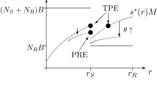
ri≡ 1 B ¯ R−C pi +C −1, i∈ {S, R} (ri>0 fori∈ {S, R}).8 The demand for capital is
D(r) = ⎧ ⎪ ⎪ ⎪ ⎨ ⎪ ⎪ ⎪ ⎩ (NS+NR)B; r≤rS NRB; rS < r≤rR 0; rR< r . (2)
The average success probability in the pool of credit applicants is p for r ≤ rS and pR for rS <
r ≤ rR. Denote the (random) return on lending at rate r in state s as i(r). This function will be determined below. Since the revenue from lending is passed through completely, the consumers solve max s : (y−s)1−θ 1−θ +δE {[1 +i(r)]s}1−θ 1−θ
by choosing an appropriate level of savings s. Let
ˆ R(r)≡E [1 +i(r)]1−θ . (3) Optimal saving is s= y 1 +δ−1θRˆ(r)−1θ ≡s ∗(r) (4)
8The variances of safe firms’ profit and their repayment to lenders are p
S(1−pS)[RS −(1 +r)B+C]2 and pS(1−pS)[(1 +r)B−C], respectively. Atr =rS, the ratio of the variances is [C/( ¯R−C)]2 and exceeds unity if C >R/¯ 2, i.e., if collateral does not fall short of half of the expected project payoff. Similarly, the ratio of the variance of risky firms’ profit to repayment atr=rS
pS−pR pR ¯ R+C ¯ R−C 2
exceeds unity under the weaker conditionC >[1−pS/(2pR)] ¯R. This confirms the assertion that for well-collateralized credit, firm owners bear the bulk of the risk created by their investments at an equilibrium with interest raterS, even though the return on lending is not safe either. If expected profit is a modest percentage of expected project payoff and, hence, of expected repayment, a comparison in terms of coefficients of variation reinforces this conclusion.
(0< s∗(r)< y), and the indirect utility function is u(y−s∗(r)) +δE{u([1 +i(r)]s∗(r))}= y 1−θ 1−θ 1 +δ1θRˆ(r)1θ θ ≡v(r). (5) From (4), the total supply of capital by a measure M of consumers facing the stochastic return profilei(r) (yet to be determined) is
S(r, M) =s∗(r)M. (6)
For the sake of brevity, we focus attention on model specifications such that
NRB < S(rS, M)<(NS+NR)B. (7)
That is, the supply of capital at interest rate rS is sufficient to carry out the risky projects but not all projects. This assumption rules out single-price market clearing equilibria (with or without adverse selection) and thus allows us to focus on the two most interesting types of equilibria: pure credit rationing equilibrium and two-price equilibrium. A pure rationing equilibrium prevails when there is positive excess demand for capital but there is no interest rate that implies a more favorable return distribution for the consumers. LetX denote the quantity of capital channeled from lenders to borrowers.
Definition 1: (r1, X) is a pure rationing equilibrium (PRE) if
→ X =S(r1, M)< D(r1),
→ there is no r such that v(r)> v(r1).
A two-price equilibrium entails that credit is given at two different interest ratesr1 and r2 (> r1),
with positive excess demand at the lower rate r1 and equality of supply and residual demand at the higher rate r2. To qualify as an equilibrium, the two interest rates have to provide consumers
with the same level of indirect utility. Moreover, interest rates at which there is positive residual demand (i.e., r < r2) must be no more favorable to consumers than r1 and r2. Let M1 (> 0) and M2 = M −M1 (> 0) denote the measures of consumers giving credit and X1 and X2 the
quantities of capital channelled from lenders to borrowers at r1 and r2, respectively. Denote the residual demand at r2 as ˜D2.
Definition 2: (r1, r2, M1, M2, X1, X2) with r2 > r1 is a two-price equilibrium (TPE) if
→ v(r1) =v(r2),
→ X1 =S(r1, M1)< D(r1),
→ X2 =S(r2, M2) = ˜D2,
-r rS rR 6 C B −1 iF(r) iS/F(r) iR(r) iR(r) iS(r) i(r)
Figure 1: Return function
In the original SW model, pure credit rationing cannot arise in equilibrium; if there is excess demand at rS but not at rR, as stipulated in (7), the equilibrium is a TPE (see Coco, 1997, Arnold and Riley, 2009, and Appendix A.1). Our first main result states that, given the presence of aggregate risk and risk-averse suppliers of capital, a PRE can arise: a PRE exists whenever there is not a TPE (except in the measure-zero event v(rR) =v(rS)):
Proposition 1: Let (7) hold. (a) Ifv(rR)< v(rS), there is a PRE and not a TPE. (b) Ifv(rR)> v(rS), there is a TPE and not a PRE. (c) If v(rR) =v(rS), there are a TPE and a PRE.
Proof: The crucial observation is thatS(r, M) (for given M) and v(r) move in the same direction asr changes. This follows immediately from (4)-(6): r affectsS(r, M) and v(r) only via ˆR(r), and both functions increase when ˆR(r) rises. From (3),
ˆ
R(r) = (1−θ)E
[1 +i(r)]−θi(r) (8) whenever i(r) exists. Let is(r) denote the return on lending in state s:9
⎛ ⎜ ⎜ ⎜ ⎝ iR(r) iS(r) iF(r) ⎞ ⎟ ⎟ ⎟ ⎠= ⎛ ⎜ ⎜ ⎜ ⎝ r λr+ (1−λ) C B −1 C B −1 ⎞ ⎟ ⎟ ⎟ ⎠, r ≤rS, (9) and ⎛ ⎝ iR(r) iS/F(r) ⎞ ⎠= ⎛ ⎝ r C B −1 ⎞ ⎠, rS< r≤rR (10)
(see Figure 1). Both forr < rSand forrS< r < rR, we haveis(r)≥0 in all states and strict inequal-ity for some states. It follows from (8) that ˆR(r)>0 and, therefore, (s∗)(r)>0,∂S(r, M)/∂r >0, and v(r) >0 for r < rS and for rS < r < rR. For r > rS, let Δ(r) denote the difference between
-r rR rS -r rR 6 rS v(r) (NS+NR)B NRB u s∗(r)M 6 u Figure 2: PRE ˆ R(r) and ˆR(rS): Δ(r)≡Rˆ(r)−Rˆ(rS), r > rS. (11) Using (3), (9), and (10), one obtains
Δ(r) = −(pS−pR) λ(1 +rS) + (1−λ)C B 1−θ − C B 1−θ +pR (1 +r)1−θ−(1 +rS)1−θ . (12)
Let ε > 0 and ε → 0. As the last term in square brackets goes to zero, while the term in braces does not (since rS >0 > C/B−1), we have limε>0,ε→0Δ(rS+ε)< 0. That is, ˆR(r) and, hence,
s∗(r),S(r, M), and v(r) jump downward at rS. Thus, bothS(r, M) (for given M) andv(r) attain their respective global maxima on the interval [0, rR] either atrS or at rR. The two constellations
consistent with (7) are illustrated in Figures 2 and 3 (evidently, parameter combinations giving rise to either case exist, as will be illustrated by means of example below).
(a) In Figure 2, S(r, M) and v(r) attain their (unique) respective maxima at rS. (rS, S(rS, M)) is
a PRE. Since v(rS)> v(r1) andrS< r2 wheneverv(r1) =v(r2) for two interest rates r1 and r2, a TPE does not exist.
(b) In Figure 3, S(r, M) and v(r) attain their (unique) maxima at rR. In this case, a PRE does not exist. For whenever there is positive excess demand at r (< rR), the second condition in the
definition of a PRE is violated: v(rR) > v(r). Let r1 = rS. There exists an interest rate r2 > r1
such thatv(r2) =v(r1). Let X1 and X2 be determined by
X1= NSN+NR
-r rR rS -r rR 6 v(r) (NS+NR)B NRB s∗(r)M 6 u u r2 rS r2 u u Figure 3: TPE
and M1 = X1/s∗(r1) (> 0) and M2 =X2/s∗(r2) (>0). From (5), v(r2) = v(r1) implies ˆR(r2) =
ˆ
R(r1). From (4), it follows that s∗(r2) =s∗(r1). Using (6) and (13), it follows from the definitions of M1 and M2 that M1+M2=M. The residual demand at r2 is
˜ D2 = 1− X1 (NS+NR)B NRB. (14)
It is straightforward to check that (r1, r2, M1, M2, X1, X2), thus defined, is a TPE: by construction, v(r1) = v(r2); from (6) and M1 =X1/s∗(r1), X1 =S(r1, M1); fromM1 < M,∂S(r, M)/∂M >0,
r1 = rS, and (7), S(r1, M1) < D(r1); from (6) and M2 = X2/s∗(r2), X2 = S(r2, M2); from (13) and (14) together with (6) andM2 =X2/s∗(r2), S(r2, M2) = ˜D2 (=−(NR/NS)S(r1, M) + (NS+
NR)(NR/NS)B); by construction,v(r)≤v(r2) for allr < r2.
(c) The proofs that (rS, S(rS, M)) is a PRE in case (a) and (r1, r2, M1, M2, X1, X2) is a TPE in
case (b) also go through whenv(rS) =v(rR). ||
The multiplicity of equilibria in case (c) is not by itself remarkable, as v(rS) =v(rR) is a
measure-zero event.10 We will come back to this case, however, when we compare welfare levels in the two types of equilibria. For now, the important point is that aggregate risk makes the emergence of a PRE possible.11
As a numerical example, let the model parameters be given by:
10One could avoid this multiplicity by making the inequality in the second condition of Definition 1 weak. 11Since r
S is the single equilibrium interest rate in a PRE, the considerations of who bears how much risk in footnote 8 apply. In a TPE, the same considerations apply for safe firms and for risky firms which get credit atrS. For risky firms that receive credit atr2, the ratio of the variances of profit and repayment is ([(1−λ)(pS−pR)C− pSR¯]/{[pR+λ(pS−pR)]C})2 and exceeds unity if C >{pS/[(1−2λ)(pS−pR)−pR]}R¯.
y M θ δ B pS pR R¯ C NS NR
10 3,000 0.5 0.95 100 0.9 0.8 110 80 100 100
Safe and risky firms apply for credit up to interest ratesrS= 13.33% andrR= 17.5%, respectively.
At rS, each consumer supplies s(rS) = 4.9369 units of capital, so the total supply of capital is 14,810.6541 (= S(rS, M)). Since it is higher than 10,000 (= NRB) and lower than 20,000 (=
(NS +NR)B), condition (7) is satisfied. As Δ(rR) = 0.0066 >0, the equilibrium is a TPE. The consumers’ indirect utility isv(rS) = 8.8883. A measure 96.2131 of randomly selected firms receive
a loan at 13.33% interest, and the 51.8935 risky firms rationed at this interest receive a loan at 15.71% interest.
4
Risk aversion and rationing
In a PRE, since rationing is necessarily random, the proportion of realized projects which are risky is equal to the proportion of risky firms in the total population of firms (i.e., 1−λ). The presence of rationing means that some risky firms do not get funds. In a TPE, by contrast, all risky projects are carried out, which makes the return profile less attractive from the risk-averse lenders’ point of view. This suggests that a PRE is more likely to emerge as the lenders’ degree of relative risk aversion rises. The present section gives a precise statement of this proposition.
Within the framework used so far we encounter the familiar problem that both relative risk aver-sion and the preference for intertemporal consumption smoothing are parameterized by the same parameterθ. So in order to appropriately address the question of which type of equilibrium emerges under what degree of risk aversion, we generalize the analysis by following Selden’s (1978) OCE approach. Let ˆc2 be the certainty equivalent (CE) corresponding to the period utility function introduced in (1): ˆ c12−θ 1−θ =E c12−θ 1−θ , θ >0, θ= 1 (15)
(we now allow for θ >1).12 Households’ utility is given by
u(c1,cˆ2) = c 1−η 1 1−η +δ ˆ c12−η 1−η, 0< η <1. (16) 1/η is the (intertemporal) elasticity of substitution betweenc1 and ˆc2. The model analyzed above is the special case with η=θ.
rR (NS+NR)B NRB rS -6 r u u s∗(r)M u ? TPE PRE θ↑ ? ?
Figure 4: Switch from TPE to PRE
ˆ
R(r)1/(1−θ) defined in (3) is the CE of 1 +i(r). Using this definition and c2 = [1 +i(r)]s, the CE
defined in (15) can be expressed as:
ˆ c2 =sRˆ(r)1−1θ. Households solve max s : (y−s)1−η 1−η +δ sRˆ(r)1−1θ 1−η 1−η . The solution is s= y 1 +δ−1ηRˆ(r)−1−1θ1−ηη ≡s ∗(r), (17)
and indirect utility is
v(r)≡ y 1−η 1−η 1 +δ1ηRˆ(r)1−1θ1−ηη η . (18)
Given the novel definitions of s∗(r) and v(r), define capital supply (cf. (6)) and the two types of equilibria as before. Our first task is to generalize Proposition 1:
Proposition 2: The assertion of Proposition 1 also holds true in the OCE framework.
Proof: The crucial observation is that, as before, changes in the interest rate move S(r, M) and v(r) in the same direction, as is evident from (17) and (18). From (3),
dRˆ(r)1−1θ dr = ˆR(r) θ 1−θE [1 +i(r)]−θi(r) .
Equations (9) and (10) hold true without modification. So for all r < rS and rS < r < rR, we haved[ ˆR(r)1/(1−θ)]/dr >0 and a fortiori (s∗)(r)>0 (from (17)),∂S(r, M)/∂r >0 (from (6)), and v(r) > 0 (from (18)). Since (3), (9), and (10) are unchanged, Δ(r) defined in (11) satisfies (12). For θ < 1, the arguments put forward in the proof of Proposition 1 prove ˆR(rS+ε) <Rˆ(rS) for
ε positive and small. Hence, ˆR(rS+ε)1/(1−θ) <Rˆ(rS)1/(1−θ). From (6), (17), and (18), it follows thatS(r, M) and v(r) jump downward as r rises above rS. Forθ >1, the term in braces in (12) is
negative, so limε>0,ε→0Δ(rS+ε)>0, i.e., ˆR(rS+ε)>Rˆ(rS) forεpositive and small. As before, this implies ˆR(rS +ε)1/(1−θ) < Rˆ(rS)1/(1−θ), so that, in this case also, S(r, M) and v(r) display
downward discontinuities at rS. This proves that both S(r, M) and v(r) attain their respective
maxima either at rS or at rR. Under the maintained assumption (7), the remainder of the proof
runs parallel to the proof of Proposition 1. ||
We are now in a position to give a precise statement of the proposition that higher risk aversion makes the emergence of a PRE more likely:
Proposition 3:Starting from a TPE, as the degree of relative risk aversionθrises and (7) remains satisfied, a PRE emerges.
Proof:The proof consists of two steps. (a) Increases inθreduces∗(r). (b) Forθlarge enough,s∗(r) andv(r) attain their maxima atrS. Thus, starting from a TPE, as risk aversion becomes stronger,
the capital supply schedule shifts downward, and at some point the maximum will occur atrS and
a PRE emerges, provided that (7) is still valid (see Figure 4).
(a) From (17), as noted by Basu und Ghosh (1993, p. 121), a decrease in the CE ˆR(r)1/(1−θ) reduces s∗(r). So we have to prove that an increase inθreduces ˆR(r)1/(1−θ)or, equivalently, ln[ ˆR(r)1/(1−θ)]. From (3) (suppressing the argument of the functions ˆR(r) and i(r)),
∂ ln ˆ R1−1θ ∂θ = 1 (1−θ)2 1 E[(1 +i)1−θ] ·E (1 +i)1−θ ln{E[ (1 +i)1−θ]} −E (1 +i)1−θln (1 +i)1−θ . Since (1 +i)1−θln[(1 +i)1−θ] is a strictly convex function of the random variable (1 +i)1−θ, the derivative is negative by virtue of Jensen’s inequality.
(b) From (12), Δ(rR) = C B 1−θ⎧⎨ ⎩−(pS−pR) ⎡ ⎣ λ1 +CrS B + 1−λ 1−θ −1 ⎤ ⎦ +pR ⎡ ⎣ 1 +rR C B 1−θ − 1 +rS C B 1−θ⎤ ⎦ ⎫ ⎬ ⎭.
SinceC/B <1+rS <1+rR, asθgrows large (in particular larger than one), the power terms inside the braces become arbitrarily small, so Δ(rR)>0. From (11), ˆR(rR)>Rˆ(rS) and ˆR(rR)1/(1−θ) <
ˆ
R(rS)1/(1−θ). From (17), it follows thats∗(r) attains its maximum at rS. || The example considered below shows that there exist model specifications such that a switch from a TPE to a PRE occurs. More generally, the following condition is sufficient to ensure that (7)
remains valid as θrises: NRB < y 1 +δ−1ηC B −1−η η M. (19)
i(rS) ≥ C/B −1 in all states of nature with strict inequality in some state of nature. Hence,
ˆ
R(rS)1/(1−θ)> C/B. From (6) and (17), S(rS, M) exceeds the term on the right-hand side of (19) for all θ, so NRB < S(rS, M). The validity of the second inequality in (7) follows from the fact
that it is satisfied in the TPE and S(rS, M) becomes smaller as θ increases (step (a) in the proof
of Proposition 3).
In the numerical example introduced at the end of the preceding section (which implicitly assumes θ = η = 0.5), the critical value for θ, above which the equilibrium is a PRE, is 2.5435. If, for instance, θ = 3, we have Δ(rR) = 0.0058. The single equilibrium interest rate is rS = 13.33%,
indirect utility is v(rS) = 8.8516. The supply of capital is 14,684.1058, so 53.1589 (or 26.58%) of the borrowers are rationed.
Another way of analyzing the impact of portfolio risk on the nature of equilibrium is to com-pare the model with correlated payoffs to the (identically parameterized) model with independent payoffs. Since rationing cannot arise in the model with uncorrelated risks, it follows immediately from Propositions 1 and 2 that the introduction of correlated risks (holding everything else equal) potentially causes rationing. Details are in Appendix A.1.
5
Inefficiency of a two-price equilibrium
From a welfare point of view, a TPE is particularly unattractive. For even leaving aside the question of whether total investment is at its optimal level, it is precisely the risky projects, disliked by the risk-averse lenders, which have a one-hundred percent chance of being financed. In the present section, we show that, as a consequence, a change in a model parameters that gives rise to a switch from a TPE to a PRE has a discontinuous positive impact on welfare. Coco (1997, pp. 12-13) arrives at the same conclusion under the assumption that riskier projects have lower expected (uncorrelated) returns and concludes that a usury law that prevents lenders from attracting risky borrowers at high interest rates raises welfare. This conclusion naturally carries over to our set-up with non-diversifiable risk and risk-averse lenders.13
Proposition 4:A parameter change that leads to a switch from a TPE to a PRE has a continuous effect on household utility but leads to a discontinuous increase in aggregate profit.
-λ 6 λ− λ+ TPE PRE -λ X1(1−λ) S(rS,M) B (1−λ) v(rS) 6 ·πR(rS) Δ(rR) λ− λ+ ·πR(rS) λ λ
Figure 5: Welfare effect of a switch from TPE to PRE (θ >1)
Proof: The proof consists of two steps. We consider first (a) the knife-edge case v(rS) = v(rR), in
which both a PRE and a TPE exist, and then (b) a small change in a parameter that leads to a switch from a TPE to a PRE.
(a) Consider the model with OCE preferences and suppose parameters are such thatv(rS) =v(rR), i.e., Δ(rR) = 0. From part (c) of Proposition 1 and Proposition 2, (rS, S(rS, M)) is a PRE, and
there is also a TPE withr2 =rR. Households’ indirect utility isv(rS) in both equilibria. The mass of projects carried out in equilibrium S(rS, M)/B is also the same in both equilibria. But while
in the PRE the loan rate is rS for all borrowers who get funds, some borrowers have to pay the
interest raterRin the TPE. This is the price firms have to pay in order to make households finance riskier projects. Total expected firm profit in the TPE is
X1
B (1−λ)πR(rS)
(where use is made of πS(rS) = 0 and πR(r2) =πR(rR) = 0). This compares with aggregate profit
S(rS, M)
B (1−λ)πR(rS)
in a PRE (where use is made of πS(rS) = 0). SinceX1 < S(rS, M), expected profit is strictly less
in the TPE.
(b) Ifθ >1, a switch from a TPE to a PRE occurs when Δ(rR) changes from negative to positive, and vice versa forθ <1. Consider model parameters (B, C, pS, pR, λ) = (B, C, pS, pR, λ) such that
Δ(rR) (i.e., dΔ(rR)/da = 0 for (B, C, pS, pR, λ) = (B, C, pS, pR, λ)). Without loss of generality, let dΔ(rR)/da >0 (if the reverse inequality holds true, consider parameter −a). For instance, let
a=λand θ >1: from (12), dΔ(r)/dλ >0 forθ >1 (see Figure 5). For θ >1, when the parameter rises froma−εto a+ε(εpositive and small), Δ(rR) turns from negative to positive and a PRE replaces a TPE, and vice versa forθ <1. From the analysis in the preceding section, it is clear that this is the only way a change in a parameter can bring about a switch from a TPE to PRE. From (3), (9), and (18), v(rS) is a continuous function of model parameters. From step (a), aggregate
profit jumps upward. ||
As pointed out by Coco (1997), this special inefficiency of a TPE can be avoided by imposing an upper bound ¯r on the set of admissible interest rates:
Proposition 5: If the equilibrium is a TPE, imposing an interest rate ceiling r¯∈ (rS, r2) raises
welfare.
Proof: Define a PRE with an interest ceiling as in Definition 1 except that we add the condition r1 ≤ r¯. The condition r ≤ r¯ rules out the existence of a TPE, for v(rS) exceeds v(r) for any
admissible pair of interest rates which yield the same expected utility. (rS, S(rS, M)) is a PRE with interest ceiling, since v(r)< v(rS) for all r≤r¯,r=rS. ||
To illustrate the assertions of Propositions 4 and 5, we modify our running example such thatθ is close to the critical value above which a PRE emerges:
y M η θ δ B pS pR R¯ C NS NR
10 3,000 0.5 2.55 0.95 100 0.9 0.8 110 80 99 101
We also changed the numbers of safe and risky firms slightly, but will return to the original values in a second. At interest rate rS = 13.33%, each household saves s∗(rS) = 4.9029, so the supply of capital is 14,708.7000. As demand drops from 20,000 to 10,100 at rS, condition (7) is satisfied.
The critical value for θ above which there is a PRE is 2.5720, so the equilibrium is a TPE with r2 = 17.47% (which can also be inferred from Δ(rR) = −0.0002 and θ > 1). Indirect utility and aggregate profit are v(rS) =v(r2) = 8.8587 and 157.8703, respectively. Now, let NS =NR = 100,
holding all other parameters fixed, so that λ rises from 49.5% to 50%. Since θ is now above the critical value 2.5435 (Δ(rR) = 6·10−5is positive), a PRE emerges. Indirect utility rises only slightly
(tov(rS) = 8.8591), but aggregate profit soars by more than 50% to 245.1701. In the former case, with 99 safe and 101 risky firms, consider the imposition of an interest rate ceiling ¯rbetween 13.34% and 15.70%. The equilibrium becomes a PRE with 13.33% interest. Borrower expected utility is
(v(rS) =) 8.8587, as in the TPE without the interest ceiling. But aggregate firm profit rises from 157.8703 to ((X/B)(1−λ)πR(rS) =) 247.5964.
6
Optimum investment
A TPE is “more inefficient” than a PRE, but even a PRE entails inefficient risk sharing. This is because firms’ collateral is a potential hedge against households’ period-2 consumption risk, but is not used completely in order to insure consumers in equilibrium, as firms which do not invest or whose projects succeed keep their collateral.14 This section characterizes the optimal solution of the model, with efficient risk sharing, and addresses the question of whether the market brings forth too little or too much investment.
For the sake of simplicity, we return to the expected utility setup. In the main text, we maintain the assumption that information is asymmetric: whennprojects are carried out,λnturn out to be safe and (1−λ)nrisky. We assume that the firms’ collateral can only be consumed in the second period. The constrained-efficient solution maximizes household expected utility for a given level β of each firm owners’ expected utility by a suitable choice of investment and state-contingent consumption levels. We show that under-investment occurs, as one might expect, for high levels ofβ and for low values of collateral. However, since decreases inβ reduce the need to invest in order to achieve the firm owners’ given level of expected utility and increases in collateral expand the pool of resources available for period-2 consumption, equilibrium over-investment can arise for low values of β and large values of collateral. (The first-best case, in which the planner can distinguish safe from risky projects, is analyzed in Appendix A.2.)
Suppose all firm owners receive the same levels of consumption in period 2, irrespective of whether their project is realized or not. Let αs denote the firm owners’ consumption level in state s ∈ {R, S, F}. Since firm owners are risk-neutral, we can assume without loss of generality that their expected utility equals expected consumption, so the constraint that they receive a given level β (≥0) of expected utility becomes
pRαR+ (pS−pR)αS+ (1−pS)αF =β. (20)
In equilibrium, a firm owner’s expected consumption isC+πi(r) if he takes a loan at interest rate
r and carries out his investment project (of type i) and C otherwise. So if, for instance, β equals the sum of collateral and expected equilibrium profit per firm owner, then the firm owners are as
well-off in the CO as in the market equilibrium. Let m ≡(NS +NR)/M denote the “number” of firms per household and c2s household consumption in state s. Then,
⎛ ⎜ ⎜ ⎜ ⎝ c2R c2S c2F ⎞ ⎟ ⎟ ⎟ ⎠= ⎛ ⎜ ⎜ ⎜ ⎝ m(C−αR) +λRS+(1B−λ)RRs m(C−αS) +λRS B s m(C−αF) ⎞ ⎟ ⎟ ⎟ ⎠. (21)
The level of investment per householdsis bounded above by the minimum ofmBandy, i.e., either by the amount of investment opportunities or by disposable income. For the sake of brevity, we restrict attention on the case in whichM y is sufficiently large to finance all investment projects:
mB ≤y.
The maximum attainable expected utility for firm owners is thenβ =C+ ¯R(achieved withs=mB and c2s= 0 for s∈ {R, S, F}).
Definition 3:Givenβ ∈[0, C+ ¯R],(c1, s, c2R, c2S, c2F, αR, αS, αF)is aconstrained optimum (CO)
if it maximizes (1) subject to the constraints s≤mB, c1=y−s, (20), (21), and non-negativity of
each component.
Since (1) is continuous and the set of vectors which satisfy the constraints is non-empty and compact, a CO exists. Since households are risk-averse and firm owners are risk-neutral, household consumption is equalized across all states in which firm owners’ consumption is positive in a CO.15 For future reference, notice that period-2 household consumption is the same when all projects succeed or only the safe projects succeed (i.e., c2R=c2S) if
αR−αS = (1−mBλ)RRs. (22)
Similarly, c2S =c2F if
αS−αF = λRS
mBs. (23)
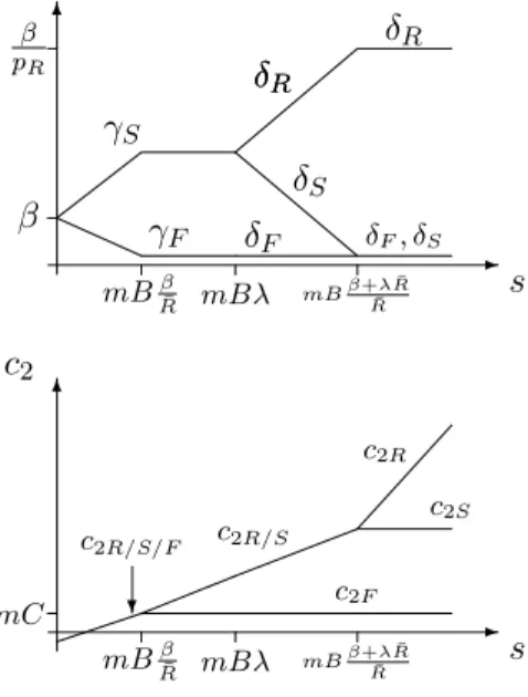
We have to distinguish three different cases, arising dependent on the choice of investment s. (a) For mBβ−¯C R ≤s≤mB β ¯ R, (24)
sis sufficiently low and the share of investment returns in total wealth is sufficiently small so that it is possible to equalize households’ period-2 consumption across all three states. Solving (20), (22),
15If households consume different quantities in two statess ands, say, their marginal rate of substitution differs fromps/ps, which is the firm owners’ marginal rate of substitution. So if the firm owners’ consumption is positive in both states, there is scope for a mutually beneficial reallocation of resources.
6 s 6 s mBβ ¯ R mB(1−βλ) ¯R αR αS αF mC m!C+1−λλpβ S " c2F c2R/S c2R c2S β β pR -mBβ ¯ R mB(1−βλ) ¯R c2R/S/F ? 6 -s mBβ ¯ R mB β (1−λ) ¯R ν(s) s∗∗
Figure 6: Consumption levels with optimal risk sharing under asymmetric information
and (23) for the αs’s and substituting into (21) gives:
⎛ ⎜ ⎜ ⎜ ⎝ αR αS αF ⎞ ⎟ ⎟ ⎟ ⎠= ⎛ ⎜ ⎜ ⎜ ⎝ β+λRS+(1mB−λ)RR−R¯s β+λRS−R¯ mB s β−mBR¯ s ⎞ ⎟ ⎟ ⎟ ⎠ and c2R/S/F =m(C−β) + ¯ R Bs (25)
(consumers’ and firm owners’ state-contingent consumption levels in this and the following two cases are illustrated in the upper two panels of Figure 6). If the first inequality in (24) is violated, then the returns on investment are insufficient so as to satisfy (20). When the second inequality in (24) is violated, the non-negativity αF ≥ 0 does not hold, i.e., the firm owners’ risk bearing capacity in the state when all projects fail is exhausted.
(b) Second, consider investment levels
mBβ¯
R ≤s≤mB β
(1−λ) ¯R. (26)
and αF = 0, we obtain: ⎛ ⎜ ⎜ ⎜ ⎝ αR αS αF ⎞ ⎟ ⎟ ⎟ ⎠= ⎛ ⎜ ⎜ ⎜ ⎝ 1 pS β+(1−λ)pS(mBRR−RS)s 1 pS β−(1−mBλ) ¯Rs 0 ⎞ ⎟ ⎟ ⎟ ⎠ and ⎛ ⎝ c2R/S c2F ⎞ ⎠= ⎛ ⎝ m C−pβS +RS B s mC ⎞ ⎠. (27) (c) Finally, for mB β (1−λ) ¯R ≤s, (28)
c2R exceeds c2S and c2F even if R is the only state in which firm owners consume:
⎛ ⎝ αR αS/F ⎞ ⎠= ⎛ ⎝ pβR 0 ⎞ ⎠. and ⎛ ⎜ ⎜ ⎜ ⎝ c2R c2S c2F ⎞ ⎟ ⎟ ⎟ ⎠= ⎛ ⎜ ⎜ ⎜ ⎝ m C−pβR +λRS+(1B−λ)RRs mC+λRS B s mC ⎞ ⎟ ⎟ ⎟ ⎠. (29)
Substitutingc1 =y−sandc2sfrom (25), (27), and (29) into (1) gives households’ expected utility as
a functionν(s) of salone. The level of investment in a CO iss∗∗= arg maxsν(s) s.t.: 0≤s≤mB. The function ν(s) is strictly concave (see the lower panel of Figure (6)). This follows from the fact that if two (c1, s, c2R, c2S, c2F, αR, αS, αF) satisfy the constraints in Definition 3, then a convex
combination also satisfies these constraints (because of linearity of the constraints) and yields higher expected utility (because of strict concavity of the function in (1) in (c1, c2R, c2S, c2F)).ν(s) is continuous and it is differentiable in the interior of the intervals in (24), (26), and (28):
ν(s)+(y−s)−θ= ⎧ ⎪ ⎪ ⎪ ⎪ ⎪ ⎪ ⎪ ⎨ ⎪ ⎪ ⎪ ⎪ ⎪ ⎪ ⎪ ⎩ δR¯ B m(C−β) +BR¯s −θ ; mBβ−R¯C < s < mBβR¯ δR¯ B mC−pβS+RS B s −θ ; mBRβ¯ < s < mB(1−βλ) ¯R δpR[λRS+(1−λ)RR] B m C−pβR +λRS+(1B−λ)RRs −θ +δ(pS−BpR)λRS mC+λRBSs −θ ; mB(1−βλ) ¯R < s . (30) It has kinks at mBβ/R¯ and at mBβ/[(1 −λ) ¯R]. There are four possible types of solutions to s∗∗= arg maxsν(s) s.t.: 0≤s≤mB. Fors(mB)≥0, all projects are realized in the CO:s∗∗=mB. Fors(0)≤0, it is optimal not to invest at all: s∗∗= 0. Ifν(s∗∗) = 0 for somes∗∗that satisfies one of the inequalities on the right-hand side of (30), then it is optimal to invests∗∗. The final possibility
is that ν(s) attains its maximum at one of the kinks, i.e., at s∗∗ =mBβ/R¯ or mBβ/[(1−λ) ¯R]. By virtue of the theorem of the maximum, s∗∗ is a continuous function of β and C. In a CO with ν(s∗∗) = 0, investment s∗∗ increases whenβ rises orC falls. This follows from the strict concavity of ν(s) and the fact that an increase in β or a decrease in C raises ν(s) (see (30)). Optimum investment s∗∗also increases with β when it occurs at a kink ofν(s).
Depending on the model parameters β, ¯R, and λ, some or all of cases (a)-(c) arise for admissible investment levels 0≤s≤mB.
¯ R≤β:
In this case, s≤mB ≤mBβ/R¯. From (24), only case (a) can arise. It is optimal to carry out all projects (i.e., s∗∗=mB) if (ν(mB)≥0, i.e.)
β≥R¯+C− y m −B δR¯ B 1 θ .
Otherwise optimum investment satisfies the first-order condition ν(s∗∗) = 0, i.e.,
s∗∗= y− δR¯ B −1 θ m(C−β) 1 +δ−1θ ¯ R B −1−θ θ . (31)
Since β≥R¯ and ¯R > C, we have β > C. So, as noted in the discussion of case (a) above, s∗∗>0. (1−λ)R¯ ≤β<R¯:
For ssmall enough, case (a) applies. Fors=mB, (26) holds with strict inequalities, i.e., case (b) applies. From (30), it is optimal to finance all projects if
β≥R¯+pS ⎡ ⎣C−y m −B δR¯ B 1 θ⎤ ⎦.
If the right-hand side of this inequality is non-positive for C = 0, then it is optimal to realize all projects (i.e., s∗∗=mB) for C low enough, irrespective of β. If the right-hand side is positive for C = 0, s∗∗=mB becomes optimal once β is large enough. If β ≥C, zero investment is ruled out on the same grounds as before. If, on the other hand, β < C,s∗∗= 0 is optimal (i.e., ν(0)≤0) if
β ≤C− δR¯ B 1 θ y m. (32) β<(1−λ)R¯:
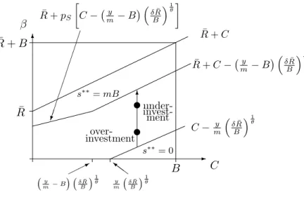
C β ¯ R+C ¯ R+C−!my −B" δBR¯ 1 θ ¯ R+pS C−!my −B" δBR¯ 1 θ y m !δR¯ B "1 θ 6 under- invest- over-investment s∗∗= 0 s∗∗=mB ¯ R !y m−B " !δR¯ B "1 θ * Z}Z C−my δR¯ B 1 θ u u B 6 ¯ R+B -ment
Figure 7: Optimum investment with asymmetric information
where now the last lines on the right-hand side of (30) are relevant. As in the preceding case,s∗∗>0 forβ ≥C, while s∗∗= 0 if (32) holds for β < C.
The results are summarized in Figure 7 (wheres∗∗< mB forβ = 0) and in:
Proposition 6: For β = 0, s∗∗ > 0 or s∗∗ = 0, depending on whether C < (y/m)(δR/B¯ )1/θ or
C≥(y/m)(δR/B¯ )1/θ, respectively. In the latter case,s∗∗>0 for β > C−(y/m)(δR/B¯ )1/θ. s∗∗ is non-decreasing in β. s∗∗=mB for β ≥R¯+C−(y/m−B)(δR/B¯ )1/θ.
In words, consumers respond to a reduction in their period-2 consumption possibilities brought about by an increase in the firm owners’ expected utility β with higher investment s∗∗. Increases in collateral C relax the constraint that firm owners receive a given level of expected utility, so optimum investments∗∗ decreases.
Having characterized both the credit market equilibrium and the CO, we can now address the question of whether there is too little or too much investment in equilibrium.
Proposition 7: In a PRE or a TPE, (a) for C small enough, there is under-investment relative to the CO for all β; (b) for C large enough, there is over-investment for sufficiently low values of
β and under-investment for sufficiently high values of β.
Proof:(a) Supposeβ =C = 0. From (28), case (c) applies for all investment levels. As noted above, β ≥C implies that the CO entails s∗∗>0. From (30),s∗∗ satisfies
s∗∗= y 1 +δ−1θ # pR λRS+(1−λ)RR B 1−θ + (pS−pR) λRS B 1−θ$−1 θ.
The term in braces exceeds pR RS B 1−θ + (pS−pR) λRS B 1−θ = ˆR(rS). (33)
So, from (4), s∗∗ > s∗(rS) for β =C = 0. C = 0 is not admissible in the equilibrium analysis (in the absence of collateral, firms would have nothing to lose from taking a credit). But both optimum investments∗∗ands∗(rS) are continuous functions ofC (fors∗(rS), this follows from the definition of rS, (3), (4), and (9)). Therefore, there is under-investment (i.e., s∗∗ > s∗(rS)) for β = 0 and C
sufficiently small. The fact that s∗∗ is non-decreasing in β and s∗(rS) (< mB) is independent ofβ
implies under-investment for all β.
(b) The fact that s∗∗= 0 for β = 0 and C ≥(y/m)(δR/B¯ )1/θ (from Proposition 6) and s∗(rS) > (1−λ)mB > 0 (from (7)) implies that there is over-investment for β = 0 and C large enough. Under-investment occurs asβ becomes sufficiently large so thats∗∗=mB. || From (4), for each C (and other model parameters except y), there exists y such that (7) is satisfied. So, from Proposition 1, for each C > 0 and β ≥ 0, there exist parameterizations of the model such that a PRE or a TPE exists. This proves that parameter combinations exist such that over-investment arises in a PRE or a TPE.
The standard under-investment result holds true if firms have little collateral and a sufficiently high weight in the planning solution. However, if there is abundant collateral a large portion of which can be reallocated to the consumers in the CO, then there is equilibrium over-investment. To illustrate this, let us return to our running example:
y M θ δ B pS pR R¯ C NS NR β
10 3,000 0.5 0.95 100 0.9 0.8 110 80 100 100 81.1737
As mentioned at the end of Section 3, there is a TPE with s∗(rS) = 4.9369 and v(rS) = 8.8883.
Total expected firm profit (X1/B)(1−λ)πR(rS) is 234.7463, so expected profit per firm owner is 1.1737. This motivates our choice of β, which equals the value of the collateral plus expected profit per capita. Optimal investment is s∗∗ = 5.0123, which is the solution to ν(s∗∗) = 0 in case (b). There is under-investment: the “number” of projects financed in the credit market equilibrium (i.e., 3,000·4.9369/100 = 148.1065) falls short of the optimum “number” (i.e., 3,000·5.0143/100 = 150.3701). Indirect utility is (ν(s∗∗) =) 8.8962. The credit market equilibrium is doubly inefficient: there is too little investment, and too large a proportion of the investment capital is dedicated to risky projects. Proposition 7 suggests that over-investment tends to arise when β falls. In fact, when β = 75 (holding everything else equal), we have s∗∗= 4.8147 <4.9369 =s∗(rS) (maximum
7
Conclusion
The present paper deviates from the common assumption in models of the credit market with asymmetric information that single-name credit risks cancel out and do not create any portfolio risk. The introduction of portfolio risk raises several interesting questions and yields several interesting results. A credit market equilibrium with pure credit rationing becomes possible. Rationing tends to arise when lenders become more risk-averse. Changes in the parameters of the credit market that lead to a switch from a two-price equilibrium to pure rationing, such as the introduction of a usury law, raise welfare. Compared to the optimal allocation of resources, the credit market equilibrium is characterized by either under-investment or over-investment, where the latter tends to occur when collateral is high and firm owners get little consumption. The implications of the model are thus much richer than the standard SW model’s, in which a non-market clearing equilibrium is generally a TPE and there is too little investment in equilibrium.
The most promising route for future research seems to be the introduction of bank capital. In the model considered here, there are no intermediaries with positive equity that could serve as a buffer against loan losses. Introducing bank capital would help make the model more complete, as one could distinguish the portions of the banks’ credit risk borne by the bank owners (the major part or all) and by the depositors (little or none at all), respectively. Another possible extension of the model would introduce lenders with heterogeneous risk attitudes, which would raise the question of the optimal allocation of risks across differently risk-averse agents. Risky collateral would shed further light on optimal risk sharing. These, and possibly further, issues can only be meaningfully addressed in a model with portfolio risk, and we are confident that our results will hold true with a small amount of bank capital, a small second group of consumers with different risk attitude, or uncertain collateral with a small variance.
Appendix A.1: Uncorrelated payoffs
This appendix compares the model with non-diversifiable risk to the standard SW model, in which single-name risks cancel out completely. We show that the introduction of correlation between project payoffs possibly causes the emergence of credit rationing and that it tends to reduce equi-librium investment. We also prove the standard equiequi-librium under-investment result for the SW model.
Call the model with non-diversifiable risk described in Sections 2 and 4 model “C”. Let “U” be the identically parameterized (SW) model that is obtained by replacing correlated with uncorrelated
payoffs. In model U, the (due to Uhlig’s, 1996, law of large numbers) safe return on lending is ˇi(r) =pr+ (1−p)(C/B−1) for r≤rS and ˇi(r) =pRr+ (1−pR)(C/B−1) forrS < r≤rR. Since consumers do not face any risk, the expected utility and OCE approaches yield the same results for U. Let ˇR(r) = [1 + ˇi(r)]1−θ. Optimal saving ˇs∗(r) is given by
ˇ s∗(r) = y 1 +δ−1ηRˇ(r)−1−1θ1−ηη (A.1) (cf. (17)). Let NRB <ˇs∗(rS)M <(NS+NR)B (A.2) (cf. (7)).
The following proposition states that the introduction of portfolio risk possibly “causes” the emer-gence of credit rationing:
Proposition A.1: (a) There exist parameters such that U does not have a PRE but C does. (b) The reverse is not true.
Proof: The return function ˇi(r) attains its unique global maximum ˇi(rR) = ¯R/B−1 at rR. Given
(A.2), similar arguments as in the proofs of Proposition 1 and 2 prove that there is a TPE and not a PRE. So U does not possess a PRE. (a) Jointly with Proposition 2, this proves the former part of the proposition. (b) The fact that U does not possess a PRE also contradicts the supposition
that C does not have a PRE but U does. ||
Another way to compare models U and C is to ask which one brings forth higher investment. The following proposition states that the introduction of portfolio risk reduces equilibrium investment:
Proposition A.2:Equilibrium investment is lower in C than in U.
Proof: From (9) and (10), E[i(r)] = ˇi(r) for allr ≤rR. Using ˇR(r) = [1 + ˇi(r)]1−θ, it follows that ˇ
R(r) ={1 +E[i(r)]}1−θ.
Jensen’s inequality implies ˆR(r) < Rˇ(r) if θ < 1 and ˆR(r) > Rˇ(r) if θ > 1. In either case, from (17) and (A.1), we have s∗(r)<sˇ∗(r) (given η < 1). That is, the presence of risk reduces optimal saving (cf. Basu and Ghosh, 1993, Proposition 1, pp. 121-2). Since (7) holds, the equilibrium of C is a TPE or a PRE, and equilibrium investment is S(rS, M) = s∗(rS)M. Since (A.2) holds, the
equilibrium of U is a TPE, and equilibrium investment is ˇs∗(rS)M. The validity of the assertion
follows froms∗(r)<ˇs∗(r). ||
De Meza and Webb (1987, Proposition 5A, pp. 287-8) argue that the equilibrium of the SW model is characterized by under-investment (irrespective of whether the credit market clears or not). They
assume that, in the optimum, the proceeds of the investment projects accrue to the consumers, but the collateral remains with the firm owners, i.e., using the notation of Section 6, β = C. Since diversification eliminates project-specific risks, safe and risky projects are equally good under these assumptions, whether there is asymmetric information or not does not matter, the first-best and second-best optima coincide. The following proposition generalizes the De Meza-Webb (1987) result:
Proposition A.3:In an equilibrium of U with s∗(r)< mB andr < rR, there is under-investment
for β ≥C.
Proof:Consider the optimal solution for model U. Given independent project risks, the safe rate of return is ¯R/B−1. Since consumers do not face any risk, we can use the notation of the model with expected utility (i.e., η=θ). Period-2 consumptionc2 is then given by the right-hand side of (25).
If optimum investment is mB, the condition s∗(r) < mB of the proposition implies that there is under-investment. So we can focus on an interior optimum. Optimum investment ˇs∗∗ is then given by the right-hand side of (31), so
ˇ s∗∗≥ y 1 +δ−1θ ¯ R B −1−θ θ (A.3)
forβ ≥C. In an equilibrium of U, as shown in the proof of Proposition A.1, we have ˇi(r)<R/B¯ −1 forr < rR. Hence, ˇR(r)<( ¯R/B)1−θ. From (A.1) with η=θ and (A.3), ˇs∗∗>ˇs∗(r). ||
If s∗(r) = mB in equilibrium, under-investment evidently cannot arise. Optimum investment is then also equal to mB. The condition r < rR rules out the special case in which the supply of
funds at the projects’ expected rate of return ¯R/B−1 is merely sufficient to financeNR projects. Equilibrium and optimum again coincide in this case.
Appendix A.2: First-best optimum
This appendix analyzes the first-best optimum that can be achieved when, contrary to what has been assumed in Section 6, it is possible to distinguish safe and risky projects.
Clearly, for M s ≤ NSB, the first-best solution entails that only safe projects are realized. For M s > NSB, allNS safe projects as well asM s/B−NS risky projects are realized. So
⎛ ⎝ c2R/S c2F ⎞ ⎠= ⎛ ⎝ m(C−γS) +RBSs m(C−γF) ⎞ ⎠,