Solidarity Behind Micro…nance
Vittoria Cerasi
Lucia Dalla Pellegrina
y V E R Y P R E L I M I N A R Y D R A F TAbstract
In this paper we analyse the role of peers’solidarity in fostering invest-ment in production in the context of micro…nance. When there is asym-metric information between lenders and borrowers on the use of borrowed funds and loans are not collateralized, there is a high chance that bor-rowers use loans for current consumption sacrifying productive projects. We study the e¤ect of solidarity in the form of insurance from a network of relatives on borrowers’ intertemporal preference for consumption and its impact on myopic behavior. The main result of the model is that solidarity might increase the share of funds devoted to investment but it might also reduce the amount of the loan in equilibrium. This result is in accordance with several features of micro-lending. We test the model using survey data from the World Bank on a sample of households in Bangladesh during the period 1991-1992. Empirical …ndings support the predictions of the model.
Key words: Micro…nance; credit rationing; social networks. JEL Classi…cation: O16, O17.
Milano-Bicocca University, Statistics Department, Via Bicocca degli Arcimboldi, 8, Milan (Italy). e-mail: [email protected]
yMilano-Bicocca University, Statistics Department, Via Bicocca degli Arcimboldi, 8,
Mi-lan (Italy), and Paolo Ba¢ Centre on Central Banking and Financial Regulation, Bocconi University, Via Roentgen, Milan (Italy). e-mail: [email protected].
1
Introduction
The most well-known strength of micro…nance, in particular of group-lending, is the ability to substitute physical collateral with other mechanisms such as as group liability, peers monitoring, social stigma, etc. designed to foster loan repayment. These mechanisms seem to be e¤ective as for instance for the three Bangladeshi Micro…nance Institutions in our empirical analysis repayment rates reach almost 95 per cent.
The problem of lack of incentives is particularly severe for Micro…nance In-stitutions (MFi, hereafter) given that they target poor people who lack physical guarantees (see for example Ghosh et al., 2000) and have a myopic approach to the future. Preference for present consumption is likely to be stronger because of high discounted rate undermining investment in productive projects with uncertain future income. This is mainly due to lower life expectancy, higher discouragement and vulnerability also due to the absence of public assistance or to the lack of savings acting as bu¤er against unexpected shocks.
One important feature ensuring the success of micro…nance is consists in ex-ploiting peers’information about the nature of each other’s projects at the stage of group formation (Ghatak, 1999 and 2000) through which MFi are able to ex-ploit the incentive to collect information by peers about each others when banks’ monitoring costs are high. Despite ex-ante peers’ information is important in explaining the success of micro…nance (Wydick, 1999; Wenner, 1995), it is not enough to avoid opportunistic behavior by the borrower when there is ex-ante moral hazard (Stiglitz, 1990), as for instance a diversion of funds from business to household needs which decreases project revenue (Menon 2003; Armendariz de Aghion and Morduch 2005, Gine et al., 2006).
The literature has suggested also social sanctions as an alternative device to overcome the problem of ex-ante moral hazard (see Besley and Coate, 1995, for a pioneering approach). In order to enhance e¤ort, ex-post punishments are imposed by individuals who are close enough to the borrower. In particular, each borrower might denounce peers’misbehavior to the village community in
order to prevent opportunistic actions. Peers can simply shun neighbors who deviate, imposing both economic and social costs.
The focus of our paper is on solidarity as a way to reduce opportunistic behavior by borrowers. Our approach is similar in the spirit to the idea of social sanctions. However solidarity has not received much attention within the micro…nance literature, besides the fact that group lending involves joint liability. There is anecdotal evidence that solidarity matters in micro…nance. O¢ ciers from several MFi, for example, seem to give much importance to such behaviors. "In the weekly meetings, FINCA employees explicitly encourage clients to develop solidarity, both to enhance their social capital as well as to monitor and enforce the loans" (Karlan, 2005).
We interpret solidarity as a form of mutual insurance between individuals, in particular relatives, who provide …nancial aid in case of negative shocks. Similarly to social sanctions1, solidarity transfers are denied to the borrower in case of misbehavior and are e¤ective if provided by those who are best informed on the borrower’s actions.
It is important to stress that not necessarily denial of solidarity comes from individuals who have been damaged by a defaulting borrower, i.e. other group members2. What is instead essential is that solidarity providers have a privileged relationship with the borrower so as to share information with her. In fact we model solidarity transfers as positively dependent on e¤ort3, which we presume
1"Social sanctions could include exclusion from other …nancial transactions (such as
in-formal insurance) or other economic or social penalties" (Nissanke, 2002). Even if the term "other …nancial transactions" may refer to future loans, it can be easily extended to solidarity transfers.
2As far as social sanctions are concerned, some authors (see for example Besley and Coate,
1995) interpret them as being imposed by other group members. Others (see for example Nissanke, 2002) state that defaulters are sub ject to e¤ective and severe sanctions by the whole community, in the form of a social stigma, not necessarily by those who are directly damaged by the default. The reasons why individuals who are not necessarily group members impose sanctions or deny solidarity could be many. For example if they belong to the same network they may be indirectly damaged through a loss of reputation. Or simply, due to their particular relationship with the borrower, they can also be driven more by socially disciplining features rather than the willingness to strike back, thus punishing even in the case they are not damaged.
3As a social insurance they fully or partially compensate the loss component due to
easily observable by individuals who are close to the borrower.
The model in the paper aims at analysing whether more solidarity reduces ex-ante moral hazard. The idea is that there are counterbalancing e¤ects. On the one hand, greater solidarity might induce borrowers to invest more in the risky project since the expected return from investment is higher due to the positive income in the default state. On the other hand, by providing insurance, solidarity might discourage e¤ort due to a softer punishment in the unlucky states.
Although solidarity, similarly to social sanctions, may be an e¢ cient mech-anism to foster investment, it might be ine¤ective to prevent strategic default –ex-post moral hazard– since it lacks the power of enforcing debt repayments once the returns on borrowers’investments have been realized (Armendariz and Morduch, 2000). We allow for this possibility by considering that the borrower’ solidarity network has access to privileged –as compared to the lender–but still imperfect information4.
Typically, dynamic incentives based on the threat of non-re…nancing are a useful instrument to avoid that such behavior takes place involving lenders’ losses. Despite not completely solving the problem of free-riding within the group and the possibility that borrowers default in the last stage of the game, the mechanism of repeated small loans designed by MFi seems to re‡ect their willingness to curb ex-post moral hazard. We do not explicitly account for this feature in the model, while we control for this in the empirical analysis.
We focus instead on another type of incentive by looking at a loan contract compatible with a non-strategic default condition for the borrower5. Therefore, in the model we endogenize the amount lent by accounting for the possibility that the lender grants loans conditionally on the borrower’s ability to access
4We assume that solidarity network can observe the full amount of invested funds without
distinguishing the share of the loan which is invested from the full amount o the loan granted. This corresponds to observing investment without knowing how muh has been borrwed.
5The Grameen II project, for example, seems to incorporate this possibility, since it is less
focused on incentives generated within the group, leaving more opportunities to concentrate also on individual lending.
intrahousehold transfers, which in turns a¤ects her e¤ort. Empirically, we look at the possibility that MFi in the dataset already use this device in order to prevent ex-post moral hazard.
Finally, we test our theoretical …ndings using data from the World Bank on a sample of households in Bangladesh during the period 1991-1992. Empirical …ndings support the predictions of the model, suggesting that when solidarity network’s …nancial capability is relatively high, more solidarity increases the share of funds devoted to investment but also reduces the amount of the loan in equilibrium. Furthermore, data predict that MFi provide loans amounts which are compatible with borrowers’non strategic default behavior.
The paper is organized as follows. In the next section we present the the-oretical model. Section 3 illustrates the dataset. In Section 4 we discuss the empirical approach and results. Section 5 concludes.
2
The Model
We consider a two-period model and three dates t = 0;1;2 where an agent maximizes her linear intertemporal utility. There are risky productive projects in the economy. The agent can decide between investing in the productive project and delay consumption or consume in the …rst period. Given that she has no initial capital to be used as input for production, she has to borrow it from a lender. No collateral is required by the lender.
The amount borrowedLcan be divided int= 1according to a sharea2[0;1] between consumptionC =aL and investment I = (1 a)L. The productive project is risky: by investing I in t = 1 each unit returns R in t = 2 with probability pand zero otherwise. Further, investing in the productive project yields a positive net present value, namelypR >1:
We assume that the cash ‡ow of the project is observable, while the share invested a is not observable to outsiders. Therefore the loan contract can be
written conditional on the project returnRbut not on the share invested. The loan contract requires the borrower to repay Rl to the lender in t= 2 only in
case of project success, while zero otherwise due to limited liability and absence of collateral.
The borrower’s choice is between immediate consumption C in t = 1 or delayed consumption in t = 2 as a result of a risky investment which might also return zero income due to failure. All individuals in the economy are risk neutral. However the agent faces an intertemporal preference rate 2 (0;1) so that delaying consumption by one unit requires a future consumption larger than one to match today sacri…ce.
Let us summarize the timing of the model as follows: Int= 0 :the agent borrowsL from the lender;
Int= 1 :the agent chooses the share of loan to consume and to invest, resp. fa;(1 a)g;
Int = 2 :the productive project returnsR or 0 and the cash ‡ow is divided according to the loan contract.
Let us analyze the intertemporal choice of the agent, given that her choice of the share invested(1 a)is not observed by the lender.
BENCHMARK CASE (no solidarity)
Assuming a linear utility in each period consumption level u(C) = C; the agent’s expected utility is
EU =C+ p(RI Rl) (1)
whereC=aLis the …rst period consumption,I= (1 a)Lis the investment in the productive project,R is the return of each unit invested in case of success andRl is the revenue to the lender in case of success. The lender is willing to
lent6, i.e.
pRl=L (2)
We can rewrite the expected utility in terms of the share of consumptionaand amount of loanL as follows:
EU =aL+ p R(1 a)L L p
For a given size of the loan L the optimal share of consumption from the agent’s point of view is given by the …rst order condition
dEU
da = 1 pR 0
When pR <1 the optimal share of consumption is a = 1: In other words, unless the intertemporal rate of substitution is close to one, that is the agent cares about the future as much as about the present, she will consume all the loan in the …rst period. This benchmark case shows that, unless the share to be invested is valued more in the future, risking in a productive project is not worth.
Now let us introduce the idea that family ties might provide an insurance policy to the agent in case of default. If this insurance is tied to the amount of the investment, since peers can observe it, future consumption through investment could be rewarded.
Agents providing solidarity transfers can observe the total amount invested by the borrowerI= (1 a)Land the return of the project in the second period so as to provide transfers only if the project fails. This implies that transfers are conditional on the amount invested, share1 a, which can be interpreted as e¤ort, on the amount lent,L, and on the …nancial capability of the solidarity network. We measure the degree of solidarity with the variable >0and de…ne total solidarity transfers asS=I = [(1 a)L] .
Solidarity might have two di¤erent e¤ects on the solution of the model. Greater solidarity, by providing insurance in the bad state, when the project
6We assume that the MFi faces competition or that it is an NGO which merely attempts
fails, might induce the agent to invest more as the income in the default state increases and therefore the expected value of the strategy of investing is greater. On the other hand, by providing insurance against the unlucky state, it might discourage e¤ort. We show under which conditions solidarity fosters investment. We carry out this analysis in two steps. Initially, we assume that the amount lent is of …xed size. However since for a given size of the loan, the borrower might behave opportunistically (by choosing a smallashe can still exploit the solidarity network when investing and the project fails), we will relax this assumption. Although the lender cannot observe the share of investment, he can anticipate this attitude and can reduce the amount of the loan in order to avoid strategic default.
Therefore as a second step we solve the model by introducing a non strategic default constraint. In this way the share of funds to be invested a¤ects the amount lent. In the reminder we separately analyze the two steps.
2.1
Fixed loan size
The agent chooses a in order to maximize her expected intertemporal utility, subject to a participation constraint of the lender. The borrower’s expected utility is:
EU=C+ fp[RI Rl] + (1 p)Sg (3)
whereS = [(1 a)L] is the solidarity transfer in case of project default. The lender’s participation constraint is given by (2) as before.
The higher is a, the higher is the …rst period consumption, while lower either the borrower’s return net of lender’s compensation,Rl, and the solidarity
transfer. Hence the overall borrower’second period consumption is lower. Note that the participation constraint of the lender only depends on the probability of success and not on the choice ofa since it is non-observable for the lender.
The …rst order condition of the maximization problem is the following: 1 = ( pR+ (1 p) [(1 a)L]1 ) (4) Rearranging (4), we obtain: a = 1 1 L " (1 p) 1 pR # 1 1 (5) Hence, assuming that 1 pR >07, it is more likely that for mildly low values of theta (0 < <1, when theta is close to 1)8 @a
@ <0, while it is more likely
for relatively high values of theta ( > 1, when theta is close to 1)9 @a @ > 0.
In all the other cases much depends on the term in squared brackets (see the Appendix for details).
In conclusion, when the amount lent is exogenous, the e¤ect of increasing sol-idarity through a higher intrahousehold network …nancial capability may bring either to an increase or to a decrease of the share of the loan which is invested depending on the capability of the solidarity network, the project return, and preference for present consumption. However, since in (5) @a
@L > 0; it turns
out that it is worth for MFi to provide borrowers with greater loans in order to increase their incentive to invest and to repay the loan. This result is in contradiction with the practice of MFi to lend small sums in general, and most importantly, with the practice of supplying di¤erent amounts according to dif-ferent characteristics, such as for example uneven access to solidarity transfers.
7From our standpoint this is the interesting case which can be justi…ed in a context of poor
borrowers since they have a low intertemporal substitution rate. If this condition does not hold it would always be convenient to invest all the loan, regardless of solidarity transfers, as shown in the benchmark case.
8Note that for very low values of we can obtain corner solutions, that isa= 1, meaning
that all the loan is consumed in the …rst period.
9Note that for very high values of ,a tends to1 1
I and we can obtain corner solutions, that isa= 0in caseIis lower than1, meaning that all the loan is invested in the …rst period. This might however not be bene…cial to the lender since the borrower could ex post decide to forego the output in order to access solidarity transfers.
2.2
Endogenous loan size and non-strategic default
incen-tives
Although from the previous analysis it appears that under some conditions solidarity might to be good in order to promote investment, it may also harm lenders. In fact, borrowers could decide to reduce their second period expected output through increasingabecause of the compensation mechanism set up by solidarity in case of default.
Suppose that in order to avoid strategic default of this kind the lender sup-plies funds according to a condition for which the borrower …nds preferable to invest and then to repay the loan rather than bene…tting from solidarity trans-fers.
In this case to the previous maximization problem of the borrower we add the following non strategic default constraint:
p[R(1 a)L Rl] (1 p) [(1 a)L]
>From the constraint we can retrieve the amount of funds borrowed condi-tional on the anticipated choice ofa:
L (1 p) (1 a) pR(1 a) 1
! 1
1
=Le (6)
Note that in order to avoid strategic default, the lender keeps the amount of the loan below a certain threshold10, Le. The constraint is binding since it is in the lender’s interest to increase the quantity of funds lent, subject to the non-strategic default constraint.
Now, as opposite to what we found in the previous version of the problem, this is compatible with the decision of MFi to provide repeated small loans to their customers. However, now the sum lent depends on the borrower’s behavior in terms of her choice ofa, which in turns depend on solidarity.
1 0Nothe that @L
@a <0if >0; @L
The …rst order condition of this problem11 still leads to (5). However now
Lis determined according to (6). ExplicitingL and rearranging we obtain:
a = 1 pR 1 (1 a) 1 pR ! 1 1
We are interested in …nding how does a vary when changes. From the Implicit Function Theorem it is possible to show (see Appendix) that, under some conditions, @a@ < 0, that is the borrower increases the share of invested funds as the solidarity network …nancial capability increases.
The analysis brings to the following conclusions. First, it is more likely that
@a
@ < 0 for relatively high values of , that is when the solidarity network
…nancial capability is high. In particular, when >1 it is always the case that
@a
@ <0. When0< <1, instead, it is more likely that @a
@ <0when departs
from0and approaches1. Moreover, in this scenario it is easier that for a given the sign of the derivative is negative whenpR and are high, that is when projects have relatively high expected returns.
Both these conditions seem to re‡ect the structure of lending in less devel-oped countries where MF programs are designed to face problems of forbidden access to banking for individuals that lack collateral but have structured and generous solidarity networks, and good projects, despite their present value is small due to their low preference for future consumption.
In the next sections we test the predictions that turn out from this theoretical analysis on households borrowing from group lending programs in Bangladesh. We also compare results from the model with endogenous loan with those ob-tained in the previous version of the model.
1 1The f.o.c. for utility maximization is the following: L + a@L @a + n
pRL+ [pRL(1 a) 1]@L@a+ (1 p) [(1 a)L] 1h L+ (1 a)@L@aio= 0
3
The Data
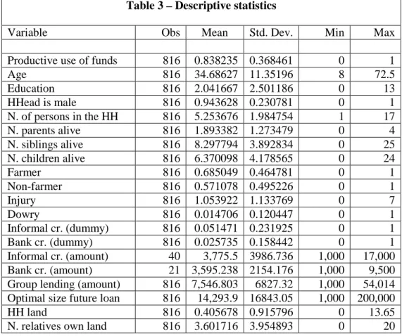
Data were collected in a survey carried out on 1,798 households in rural Bangladeshi villages by the Bangladesh Institute of Development Studies at the World Bank in 1991/9212.
The sample consists of three randomly selected villages from each of the 29 districts (thanas) surveyed. In 24 of these districts, a microcredit program (Grameen, Bangladesh Rural Advanced Committee or Bangladesh Rural De-velopment Board) had been in operation for at least three years. A total of 20 households in each village were surveyed.
Although the survey has been conducted three times during the period, here we concentrate on the …rst round (November-February), which is the most reliable setup in order to provide clear answers to our theoretical issues, since much information is missing in the remaining two.
Among all the household surveyed 816 joined group lending programs. We concentrate on these, since they better …t our theoretical setup. In particular, households who are accorded loans from the three MFi mentioned above all faced the same constant interest rate (16 per cent at the time of the survey) an are not required to provide collateral.
In fact, di¤erent objective functions and market structure of lenders (think for example about monopolistic or oligopolistic moneylenders) would complicate the theoretical framework without providing clear-cut predictions.
Our proxy for the share of invested funds is a dummy variable which takes the value of 1 when the household ex post declares that has devoted the loan to productive uses (farming or other self-employed activities).
Among the 816 households borrowing from group lending programs 83 per cent stated that they have used funds for production, while the remaining ones
1 2Although micro…nance has made further improving steps in recent years, still group
lend-ing is the core of credit services provided by institutions like the GB, BRDB or BRAC. Informal and bank credit are also granting almost the same services as in 1991/1992. Hence, in order to analyze recent issues raised in the micro…nance literature, the dataset seems not to supply aged information.
declared that they made personal use, such as dowries, food or medical expenses. Thus, on average, our variableain the model should amount to 0.17.
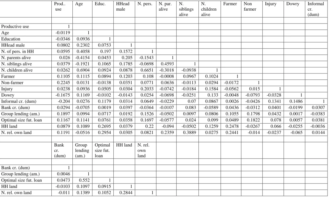
The variable which we consider eligible to capture the degree of solidarity is the intrahousehold network …nancial capability ( in the model), represented by the number of close relatives (parents and siblings) owning land. In fact, land is considered the more reliable measure of wealth in such contexts. In the dataset the number of parents and siblings owning land is 3.6, with a maximum of 20.
The amount of the actual –or ex-post–transfers received by the households is also available in the data. However, we do not use this as an independent de-terminant of the share of invested funds for two reasons. First, according to the model, ex-post transfers include the choice of the share of invested funds itself, instead of representing the potential degree of solidarity which the borrower can access. Second, from an econometric perspective, actual transfers are endoge-nous with respect to the dependent variable. Our choice is thus to use a measure of potential solidarity which is not related to unmeasurable characteristics of the household a¤ecting the share of invested funds.
Households own 0.4 acres of land on average, a fact that re‡ects the well known principle set up by the Grameen Bank and other MFi in order to select poor borrowers. This control variable is crucial to our purposes and always needs to be coupled with the number of relatives owning land in order to clean the presence of our main regressor from possible correlation with borrowers’ wealth.
Information about the type of activity carried out by the household head may be important in order to capture possible di¤erences in the project ex-pected returns (pRin the model). Since we believe that important di¤erences exist between returns from farming and non farming activities13, we build two dummies capturing this. Within the sample, 68 per cent of the household are farmers (raise crops or rear animals) while 57 per cent conduct other
non-1 3For example, due to ‡oods and adverse climate conditions, it is likely that farming has
agricultural activities. The remaining ones are non-self employed14.
Some other variables are used to gather information on the intertemporal preference rate, . The average age of the household head –who is male in 94 per cent of the cases– and his/her spouse is 34 and they attended school for slightly more than two years. On average household are made of …ve members, household head and spouse have 2 parents alive (within four), eight siblings and six children. The number of children, in particular, seems a good measure of weight accorded to future consumption (i.e. the higher the number of children, the higher is ).
In order to check the robustness of our results we also account for possible shocks occurred to household members. In fact, funds might be subtracted from productive uses in case some household member su¤ers a disease and requires medical assistance or medicines. Even in case of marriage it is possible that productive projects are foregone in order to provide dowries. The number of household members who have been hit by some injury is 1 on average, with a maximum of 7, while 1.4 per cent of the households provided their daughters with a dowry.
The presence of other sources of credit should also be controlled since it may as well account for di¤erences in the share of funds conveyed towards produc-tion. Five and two per cent of the households have been accorded loans from informal moneylenders15 and banks respectively. The average loan accorded by informal lenders amounts to 3,775 while it is 3,595 taka if loans come from banks, although the standard errors are quite high. Loans from MFi are instead 7,546 taka on average.
Finally, borrowers are asked what is the optimal loan size if they do over again. We consider this as the best available measure for the threat of non-re…nancing. Basically, the larger is the future desired loan the higher the threat.
1 4Note that in most of the cases micro…nance helps borrowers to start a new productive
activity. These are ex post data, meaning that they already encompass the productive use of funds made by households who have been accorded loans in the past.
1 5Among this category we include input suppliers, merchants, landlords, relatives and
We summarize all variables in the appendix.
4
Empirical Analysis
Given the available data, the model previously analyzed leads to estimate the following equation:
yij =rij 0+hij 1+Aij 2+ j+ ij (7)
whereiidenti…es the household, which is the unit of observation, andjrefers to the village.
yij is the productive use dummy variable, rij is the number of relatives
owning land, whilehij is the household land. Aij is a set of control variables.
Finally, j are village speci…c-e¤ects, while ij is an idiosyncratic error, such
thatE( ijjrij; hij; Aij; j) = 0:
In particular, sinceyij is a dummy, we assume that
Pij=F(Iij)
where F is the cumulative distribution function of the standard normal, andPij is the value it takes in Iij =rij 0+hij 1+Aij 2+ j, that is the
probabilityPij that yij = 1.
We use probit techniques to estimate equation (7) checking the robustness of our …ndings by changing the set of variables included in the vectorA.
4.1
Results
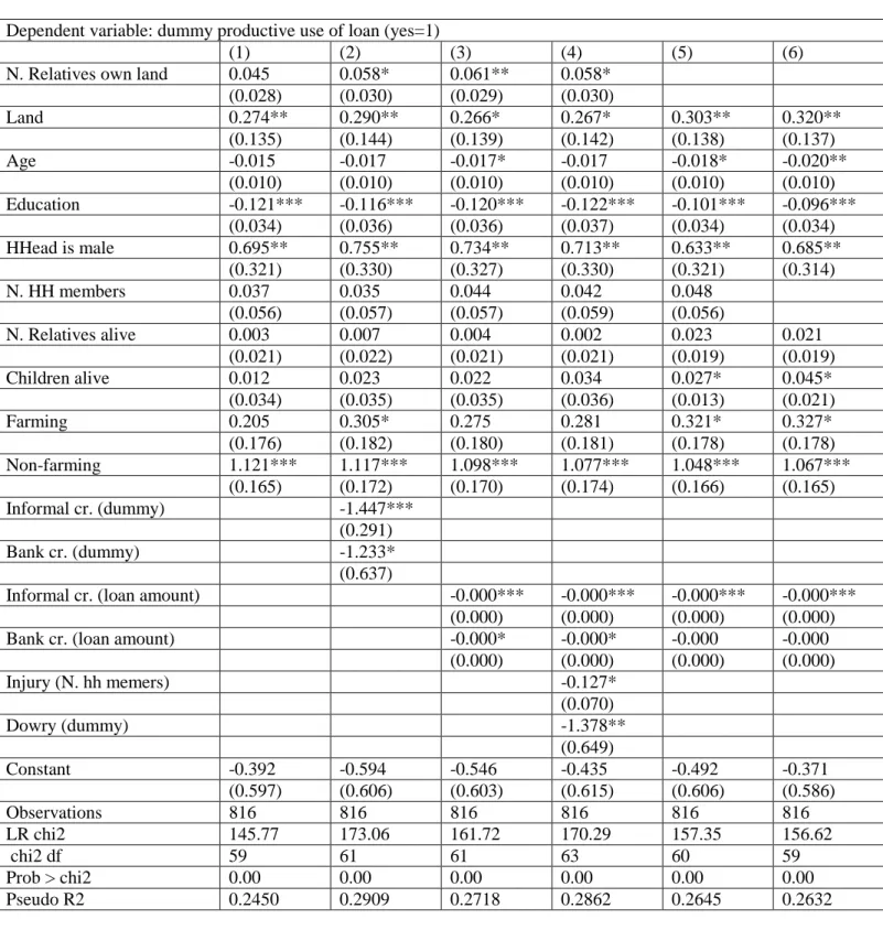
Regression output is summarized in Tables 1 and 2. Table 1 refers to the version of the model with exogenous loan amount, while Table 2 refers to the version with endogenous one. The di¤erence between the two, from an empirical standpoint, consists in controlling for the sum borrowed: we do it in the former case, while in the second we do not.
In each regression we control for household characteristics which can af-fect the use of borrowed sums, such as the average age of the household head and spouse, their education, the gender of the household head, the number of household members and the relationship network of the house measured by the number of relatives alive. In this case we separate parents and siblings from children, since the latter should better re‡ect the intertemporal preference rate of borrowers. Moreover, we always account for the main activity carried out from the household head, being this a farming or a non-farming one, and leave non self-employed as a residual class.
In particular, in the …rst column of each table we do not control for other sources of lending and possible shocks occurred to the household, which may divert funds from production. In the second column we control for the former in form of a dummy which takes the value 1 when the household also borrowed from informal lenders or banks, separating the two alternative sources. In the third column we adopt the same approach including a variable measuring the amount of loans from sources di¤erent from group lending instead of the dummy. In the fourth column we add variables capturing shocks, in the form of disease or dowry.
Columns (5) and (6) are for robustness check. Here we take the …rst basic result of column (1) and remove our main regressor, that is the number of close relatives owning land. In column (5) we do not add any substitute for this, but check whether the number of relatives alive is signi…cant. In this case it would mean that it would not be relatives’ wealth to raise the propensity to invest (1 a) but simply the relationship network, regardless of its …nancial capability. In column (6), in order to verify the same point, we also remove the number of household members, due to its possible collinearity with the number of relatives (children in particular) who are alive.
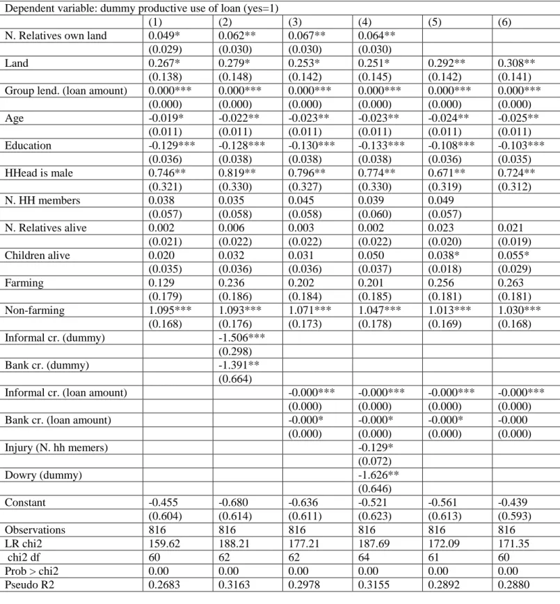
Starting from Table 1 we can observe that our measure of the solidarity network …nancial capability is signi…cant with positive sign, suggesting that when the number of relatives owning land increases the probability that the
borrower uses funds for productive activities increases.
The marginal e¤ect is on average 1.3, meaning that having one additional relative with land leads to an increase in the probability by 1.3 per cent. Consid-ering for example that the household with the higher number of landed relatives has twenty, it means that its members have a 26 per cent higher probability of devote loans to production as compared to those not having access to transfers. Our measure of household wealth, captured by land ownership, is signi…cant and with a positive sign. This is interesting, but somehow expected, as it means that when resources constraints are less binding, households do not need to use borrowed funds to consume while waiting that output materializes, hence they are more likely to invest the full loan. Moreover, this result explains why, while MFi target landless borrowers, those who are richer amongst the poor are also more likely to repay, and thus preferred by lenders.
Looking at the household characteristics, we see that younger people are more likely to increase the probability of devoting sums to productive purposes, and this should re‡ect their higher intertemporal preference rate, according to our theoretical analysis. Another result which is not surprising and has the same explanation as the previous one, is the sign of the parameter associated to the number of children. This is sometimes signi…cant, although weakly, or close to be.
The result for education is somehow surprising, since it seems that the more educated the household head and spouse the less they invest. One possible ex-planation is that highly educated household members are also more productive, and need to invest less in order to achieve the same output of less educated individuals. Another explanation could be the fact that they are richer16, de-liberately borrow for non-productive purposes, and are con…dent to being able to repay through other sources of wealth or income.
The household head being male is also a strong result, showing that male heads are more likely to invest in production rather that women, although there is not a signi…cant number of households managed by women as to exclude the
possibility that this is driven by one or a few cases only. Nonetheless, there might be several explanations for this fact, some for example linked to child rearing and education (Jackson, 1996), which are in line with some previous empirical …ndings (Pitt and Khandker, 1998; Kritikos et al., 2005).
Carrying out self-employed (farming or non-farming) activities increases the probability that funds are devoted towards production. This is somehow trivial and also an endogenous outcome, since often the purpose of group lending is to induce workers to become self-employed. However, the interesting feature is that non-farmers invest more than farmers, and it should in principle re‡ect the e¤ect of a higher expected output on the share of funds invested, as analyzed in the model. In fact, if non-agricultural activities have a higher expected output –and this is plausible given the higher probability of failure of agricultural projects in this context17–our theoretical results …nd support in the data.
Our measures of shocks are also signi…cant with the expected –negative– sign, suggesting that injuries and particularly dowries are very likely to divert funds from productive purposes, as one can observe from column (4) in each table.
As far as the other sources of lending are concerned (see all columns but (1)), it is interesting to note that their presence and amount go both in the direction of reducing the probability of investing in production. This result is de…nitely stronger for informal lending. It might be due to the high correlation of informal lending with shocks. In fact, despite we control for illness and dowries, it may be that they do not exhaust all the possible types of shocks which are faced with intrahousehold borrowing. It is interesting to note that micro…nance seems to perform better than the other two types of credit. This is consistent with empirical evidence (Dalla Pellegrina, 2008), although these results may su¤er from selection problems a¤ecting bank and informal credit in particular.
Looking at the last two columns of each regression output it can be veri…ed that what matters in order to increase the propensity to invest is the wealth
of the borrowers’ relationship network. In fact, by removing the number of relatives owning land or the number of household members from regressions we do not obtain any signi…cant increase of the parameters associated to the number of relatives who are alive18.
We also run all the regressions in Tables 1 and 2 taking account of the measure of desired future loans. Results, although not explicitly reported in the regression output, show no signi…cance of the parameter associated to this variable in case we control for the actual (current) loan amount (Table 1). The parameter, instead becomes signi…cant and positive once we remove the loan amount, suggesting that the threat of non re…nancing is e¤ective. However, the presence of this control does not a¤ect the sign and signi…cance of the number of relatives owning land.
Finally, comparing Tables 1 and 2, one can observe that the results discussed so far do not substantially di¤er if we estimate the probability of investing with or without including the amount of the loan. However, it is interesting to look at the only di¤erence, that is the sign –positive–and signi…cance of the parameter associated to the sums accorded through group lending (Table 1). This useful to verify whether it is the case that MFi exogenously accord the amount lent or loans are endogenously determined. Apart from the predictions in terms of the e¤ects of increasing solidarity19, the version of the model with exogenous loan amount stated that increasing it would lead to a lower propensity towards investing. Hence, empirical evidence contradicts this theoretical prediction leav-ing room to the possibility that the loan amount is actually endogenously de-termined as a consequence of the strategy adopted by MFi in order to prevent the borrower’strategic default.
1 8Actually, the parameter slightly increases but does not become signi…cant in any case. 1 9In the version of the model with exogenous principal these were ambiguous, meaning that
only under some conditions increasing solidarity led to an increase in the of the propensity towards investing. However, from the empirical analysis the e¤ect seems one-way, and not the result of multiple equilibria.
5
Concluding remarks
In this paper we study how solidarity may enhance investment when there is asymmetric information in credit markets and borrowers have no collateral en-dowments. Throughout the analysis, we assume that borrowers have a strong preference for current consumption, represented by low intertemporal preference rates, as is the case for less developed countries where MFi operate.
We model a situation where borrowers choose the share of funds to consume in the current period, which is complement to that invested in a productive project which returns a random output in the future. Their investment e¤ort is therefore represented by sacri…cing present consumption.
In such a framework, the impact of solidarity transfers may be in principle ambiguous. On the one hand higher transfers increase borrowers’ willingness to sacri…ce present consumption because they are provided by individuals who have information on the level of e¤ort exerted. On the other hand, they enhance myopic behaviors due to the bu¤er-e¤ect represented by solidarity in case of default.
In the theoretical part we show that when solidarity network’s …nancial capability is relatively generous, more solidarity increases the share of funds devoted to investment but also reduces the amount of the loan in equilibrium. This second e¤ect, in particular, stems from the non-strategic default devices set up by MFi in order to enforce loan repayment. These results are consistent with some typical features of MFi loans lending small sums in context where social ties are important and solidarity networks are structured and generous.
We test the model using data from the World Bank on a sample of house-holds in Bangladesh during the period 1991-1992. Empirical …ndings suggest that the probability that borrowers invest their loan in productive activities positively depends on their intrahousehold network …nancial capability, repre-sented by the number of relatives owning land, which has been selected as an exogenous measure of potential transfers. Moreover, econometric speci…cations that account for measures of the threat of non re…nancing, although signi…cant,
do not a¤ect our main results.
In conclusion, this work provides two main implications. First, it is impor-tant that MFi account not only for incentive mechanisms that lay within groups in case of joint liability but also on those relying to the borrower’s social net-work. A corollary of this is that there are instruments to enforce ex-ante good behaviors even in the case of individual lending, a point that seems particu-larly important for the Grameen II project. Second, it is possible for MFi to accord loans which are compatible with the reduction of ex-post moral hazard in the form of strategic default. By doing this, MFi also modify the structure of ex-ante incentives which become jointly determined with the amount borrowed.
References
[1] Armendáriz de Aghion B. and Morduch J., Micro…nance: Where Do We Stand? in Financial Development and Economic Growth: Explaining the Links, ed. by C. Goodhart, Macmillan/Palgrave, p. 139, 2003.
[2] Armendáriz de Aghion B. and Morduch J., Micro…nance Beyond Group Lending,Economics of Transition, Volume 8 Issue 2, pp. 401–420, 2000. [3] Dalla Pellegrina L., Micro…nance and Investment: a
Compar-ison with Bank and Informal Lending, Available at SSRN: http://ssrn.com/abstract=953231.
[4] Ghatak M., Screening by the Company You Keep: Joint Liability Lending and the Peer Selection E¤ect, The Economic Journal, Vol. 110, Issue 465, pp. 601-631, 2000.
[5] Ghatak M., Group lending, local information and peer selection, Journal of Development Economics, Vol. 60, pp. 27–50, 1999.
[6] Ghosh P., Mokherjee D. and Ray D., Credit Rationing in Developing Coun-tries: An Overview of the Theory, in D. Mokherjee and D. Ray, Readings in the Theory of Economic Development, Blackwell Publishing Company, 2000.
[7] Gine X., Jakiela P., Karlan D. S. and Morduch J., Micro…nance Games, Yale University Economic Growth Center Discussion Paper No. 936, June 2006.
[8] Jackson C., Rescuing Gender From the Poverty Trap, World Developmnt, Vol. 24, No. 3, pp. 489-504, 1996.
[9] Kritikos, A. S. and Vigenina D., Key Factors of Joint-Liability Loan Con-tracts. An Empirical Analysis, KYKLOS, Vol. 58, Issue 2, pp. 213–238, 2005.
[10] Karlan D. S., Using Experimental Economics to Measure Social Capital and Predict Financial Decisions, Yale University Economic Growth Center Discussion Paper No. 909, April 2005.
[11] Menon N., Consumption Smoothing in Micro-Credit Programs, Develop-ment and Comp Systems 0403005, EconWPA, 2004.
[12] Nissanke M., Donors’Support for Microcredit as Social Enterprise. A Criti-cal Reappraisal, Discussion Paper No. 127 United Nations University, 2002. [13] Pitt M. M. and Khandker S., The Impact of Group-Based Credit Programs on Poor Households in Bangladesh: Does the Gender of Participants Mat-ter?,Journal of Political Economy,Vol. 106, No. 5, pp. 958-996, 1998. [14] Wenner M. D., Group Credit: A Means to Improve Information Transger
and Loan Repayment Performance, Journal of Development Studies Vol. 32, Issue 2, pp. 264-81, 1995.
[15] Wydick B., Can Social Cohesion be Harnessed to Repair Market Failures? Evidence from Group Lending in Guatemala,The Economic Journal, Vol. 109, Issue 457, pp. 463 - 475, 1999.
[16] Stiglitz, J., Peer Monitoring andCredit Markets, World Bank Econ. Rev. Vol. 4, Issue 3, pp. 351–66, 1990.
Appendix
Fixed loan size
@a @ = @ 1 1 L (1 p) 1 pR 1 1 ! @ = = 1 I |{z} >0 h 1 ( 1)2 ln (1 p) 1 Rp (11) i (1 p) 1 Rp ! 1 1 | {z } >0
The term in squared brackets is negative if: (1 ) <ln 1(1Rpp)
Hence, for:
1) Very low : 0< <1; 0 < 1(1Rpp) < 1 it could be either @a@ <0 or @a
@ >0
2) Mildly low : 0< <1; 1(1Rpp)>1 always @a@ <0
3) Mildly high : >1; 0< 1(1Rpp)<1 always @a@ >0
4) Very high : >1; 1(1Rpp) >1 it could be either @a@ <0or @a@ >0
Endogenous loan size
a = 1 pR 1 (1 a) 1 pR 1 1 F(a; ; p; R; ) =a 1 + pR 1 (1 a) 1 pR 1 1 = 0
By the Implicit Function Theorem:@a@ = @F@ @F @a @F @ = @ 0 @a 1+ pR (11a) 1 pR ! 1 1 1 A @ = 1 2 2 +1 ln Rp Rap Rap Rp a+1 Rp Rap Rap Rp a+1 1 1 = = 1 ( 1)2 | {z } >0 ln (1 a)1 | {z } <0 if0< <1 >0if >1 (1 a) | {z } >0 Hence: @F@ <0if0< <1; @F@ >0 if >1 @F @a = @ 0 @a 1+ pR 1 (1 a) 1 pR ! 1 1 1 A @a =
= 1 (1 a)2(1 )[1 Rp ](1 a) Note that if >1 : @F @a = 1 (1 a)2 | {z } >0 (1 ) | {z } <0 [1 Rp ] | {z } >0 (1 a) | {z } >0 Hence: a) if >1: @F @a >0, and consequently @a @ <0 b) if0< <1 : in order for @F @a <0, such that @a @ <0, we need: (1 a)2 (1 ) [1 Rp ]<
This holds for:
Table 1 – Effect of solidarity on the use of MF loans when the loan amount is exogenously fixed
Dependent variable: dummy productive use of loan (yes=1)
(1)
(2)
(3)
(4)
(5)
(6)
N. Relatives own land
0.049*
0.062**
0.067**
0.064**
(0.029)
(0.030)
(0.030)
(0.030)
Land
0.267*
0.279*
0.253*
0.251*
0.292**
0.308**
(0.138)
(0.148)
(0.142)
(0.145)
(0.142)
(0.141)
Group lend. (loan amount)
0.000***
0.000***
0.000***
0.000***
0.000***
0.000***
(0.000)
(0.000)
(0.000)
(0.000)
(0.000)
(0.000)
Age
-0.019*
-0.022**
-0.023**
-0.023**
-0.024**
-0.025**
(0.011)
(0.011)
(0.011)
(0.011)
(0.011)
(0.011)
Education
-0.129***
-0.128***
-0.130***
-0.133***
-0.108***
-0.103***
(0.036)
(0.038)
(0.038)
(0.038)
(0.036)
(0.035)
HHead is male
0.746**
0.819**
0.796**
0.774**
0.671**
0.724**
(0.321)
(0.330)
(0.327)
(0.330)
(0.319)
(0.312)
N. HH members
0.038
0.035
0.045
0.039
0.049
(0.057)
(0.058)
(0.058)
(0.060)
(0.057)
N. Relatives alive
0.002
0.006
0.003
0.002
0.023
0.021
(0.021)
(0.022)
(0.022)
(0.022)
(0.020)
(0.019)
Children alive
0.020
0.032
0.031
0.050
0.038*
0.055*
(0.035)
(0.036)
(0.036)
(0.037)
(0.018)
(0.029)
Farming
0.129
0.236
0.202
0.201
0.256
0.263
(0.179)
(0.186)
(0.184)
(0.185)
(0.181)
(0.181)
Non-farming
1.095***
1.093***
1.071***
1.047***
1.013***
1.030***
(0.168)
(0.176)
(0.173)
(0.178)
(0.169)
(0.168)
Informal cr. (dummy)
-1.506***
(0.298)
Bank cr. (dummy)
-1.391**
(0.664)
Informal cr. (loan amount)
-0.000***
-0.000***
-0.000***
-0.000***
(0.000)
(0.000)
(0.000)
(0.000)
Bank cr. (loan amount)
-0.000*
-0.000*
-0.000*
-0.000
(0.000)
(0.000)
(0.000)
(0.000)
Injury (N. hh memers)
-0.129*
(0.072)
Dowry (dummy)
-1.626**
(0.646)
Constant
-0.455
-0.680
-0.636
-0.521
-0.561
-0.439
(0.604)
(0.614)
(0.611)
(0.623)
(0.613)
(0.593)
Observations
816
816
816
816
816
816
LR chi2
159.62
188.21
177.21
187.69
172.09
171.35
chi2 df
60
62
62
64
61
60
Prob > chi2
0.00
0.00
0.00
0.00
0.00
0.00
Pseudo R2
0.2683
0.3163
0.2978
0.3155
0.2892
0.2880
Standard errors in parentheses
significant at 10%; ** significant at 5%; *** significant at 1% Marginal effects to be computed.
All regressions have been run controlling for the optimal desired size of the loan in case of future borrowing. This measure is not significant in any specification and does not affect the sign and significance of the number of relatives owning land.
Table 2 – Effect of solidarity on the use of MF loans with endogenous loan amount
Dependent variable: dummy productive use of loan (yes=1)
(1)
(2)
(3)
(4)
(5)
(6)
N. Relatives own land
0.045
0.058*
0.061**
0.058*
(0.028)
(0.030)
(0.029)
(0.030)
Land
0.274**
0.290**
0.266*
0.267*
0.303**
0.320**
(0.135)
(0.144)
(0.139)
(0.142)
(0.138)
(0.137)
Age
-0.015
-0.017
-0.017*
-0.017
-0.018*
-0.020**
(0.010)
(0.010)
(0.010)
(0.010)
(0.010)
(0.010)
Education
-0.121***
-0.116***
-0.120***
-0.122***
-0.101***
-0.096***
(0.034)
(0.036)
(0.036)
(0.037)
(0.034)
(0.034)
HHead is male
0.695**
0.755**
0.734**
0.713**
0.633**
0.685**
(0.321)
(0.330)
(0.327)
(0.330)
(0.321)
(0.314)
N. HH members
0.037
0.035
0.044
0.042
0.048
(0.056)
(0.057)
(0.057)
(0.059)
(0.056)
N. Relatives alive
0.003
0.007
0.004
0.002
0.023
0.021
(0.021)
(0.022)
(0.021)
(0.021)
(0.019)
(0.019)
Children alive
0.012
0.023
0.022
0.034
0.027*
0.045*
(0.034)
(0.035)
(0.035)
(0.036)
(0.013)
(0.021)
Farming
0.205
0.305*
0.275
0.281
0.321*
0.327*
(0.176)
(0.182)
(0.180)
(0.181)
(0.178)
(0.178)
Non-farming
1.121***
1.117***
1.098***
1.077***
1.048***
1.067***
(0.165)
(0.172)
(0.170)
(0.174)
(0.166)
(0.165)
Informal cr. (dummy)
-1.447***
(0.291)
Bank cr. (dummy)
-1.233*
(0.637)
Informal cr. (loan amount)
-0.000***
-0.000***
-0.000***
-0.000***
(0.000)
(0.000)
(0.000)
(0.000)
Bank cr. (loan amount)
-0.000*
-0.000*
-0.000
-0.000
(0.000)
(0.000)
(0.000)
(0.000)
Injury (N. hh memers)
-0.127*
(0.070)
Dowry (dummy)
-1.378**
(0.649)
Constant
-0.392
-0.594
-0.546
-0.435
-0.492
-0.371
(0.597)
(0.606)
(0.603)
(0.615)
(0.606)
(0.586)
Observations
816
816
816
816
816
816
LR chi2
145.77
173.06
161.72
170.29
157.35
156.62
chi2 df
59
61
61
63
60
59
Prob > chi2
0.00
0.00
0.00
0.00
0.00
0.00
Pseudo R2
0.2450
0.2909
0.2718
0.2862
0.2645
0.2632
Standard errors in parentheses
significant at 10%; ** significant at 5%; *** significant at 1% Marginal effects to be computed.
All regressions have been run controlling for the optimal desired size of the loan in case of future borrowing. This measure is positive and significant in any specification but does not affect the sign and significance of the number of relatives owning land.
Table 3 – Descriptive statistics
Variable
Obs
Mean
Std. Dev.
Min
Max
Productive use of funds
816
0.838235 0.368461
0
1
Age
816
34.68627 11.35196
8
72.5
Education
816
2.041667 2.501186
0
13
HHead is male
816
0.943628 0.230781
0
1
N. of persons in the HH
816
5.253676 1.984754
1
17
N. parents alive
816
1.893382 1.273479
0
4
N. siblings alive
816
8.297794 3.892834
0
25
N. children alive
816
6.370098 4.178565
0
24
Farmer
816
0.685049 0.464781
0
1
Non-farmer
816
0.571078 0.495226
0
1
Injury
816
1.053922 1.133769
0
7
Dowry
816
0.014706 0.120447
0
1
Informal cr. (dummy)
816
0.051471 0.231925
0
1
Bank cr. (dummy)
816
0.025735 0.158442
0
1
Informal cr. (amount)
40
3,775.5 3986.736
1,000
17,000
Bank cr. (amount)
21 3,595.238 2154.176
1,000
9,500
Group lending (amount)
816 7,546.803
6827.32
1,000
54,014
Optimal size future loan
816
14,293.9 16843.05
1,000 200,000
HH land
816
0.405678 0.915796
0
13.65
Table 4 – correlations
Prod.. use
Age Educ. HHead
male N. pers. N. par. alive N. siblings alive N. children alive Farmer Non farmer
Injury Dowry Informal
cr. (dum) Productive use 1 Age -0.0119 1 Education -0.0346 0.0936 1 HHead male 0.0802 0.2302 0.0753 1 N. of pers. in HH 0.0595 0.4058 0.197 0.1572 1 N. parents alive 0.026 -0.4154 0.0453 0.205 -0.1543 1 N. siblings alive 0.0379 -0.1921 0.1065 0.1785 -0.0698 0.4593 1 N. children alive 0.0262 0.6904 0.0924 0.0878 0.6651 -0.3018 -0.0938 1 Farmer 0.1105 0.1115 0.0894 0.1203 0.108 -0.0008 0.0967 0.1024 1 Non-farmer 0.2245 0.0131 -0.0138 0.0351 0.0771 0.0636 -0.0113 0.0294 -0.0172 1 Injury 0.0238 0.0936 0.0505 0.0304 0.2033 -0.0742 -0.0184 0.1584 -0.0562 0.015 1 Dowry -0.1675 0.1169 -0.0102 -0.0143 0.0254 -0.0698 -0.0251 0.133 -0.0048 -0.0793 -0.0328 1 Informal cr. (dum) -0.204 0.0276 0.1179 0.0314 0.0649 -0.0229 0.07 0.0867 0.0026 -0.0426 0.1341 0.1486 1 Bank cr. (dum) 0.0294 -0.0705 0.0019 0.0397 -0.0364 -0.0107 0.083 -0.0589 0.0436 -0.0312 0.0401 -0.0199 0.0307
Group lending (am.) 0.1897 0.0994 0.0717 0.0192 0.1526 -0.0502 0.0097 0.0806 0.1055 0.1798 0.0432 0.0017 -0.0383
Optimal size fut. loan 0.1167 0.1141 0.0761 0.0358 0.1697 -0.0577 0.024 0.099 0.0489 0.1822 0.078 0.0057 0.0381
HH land 0.0879 0.1089 0.2695 0.0379 0.22 -0.094 -0.0502 0.1259 0.2478 -0.0267 0.066 -0.0255 -0.0036
N. rel. own land 0.1191 -0.0516 0.2954 0.0305 0.0821 0.2359 0.3889 0.0275 0.2441 -0.014 -0.0237 -0.065 0.0144
Bank cr. (dum) Group lending (am.) Optimal size fut. loan HH land N. rel. own land Bank cr. (dum) 1
Group lending (am.) 0.0046 1
Optimal size fut. loan 0.0473 0.552 1
HH land -0.0103 0.1097 0.0915 1