Nonparametric predictive inference for diagnostic test thresholds.

(1)

Durham Research Online

Deposited in DRO:

09 October 2018

Version of attached le:

Accepted Version

Peer-review status of attached le:

Peer-reviewed

Citation for published item:

Coolen-Maturi, T. and Coolen, F.P.A. and Alabdulhadi, M. (2020) 'Nonparametric predictive inference for diagnostic test thresholds.', Communications in statistics : theory and methods., 49 (3). 697-725 .

Further information on publisher's website:

https://doi.org/10.1080/03610926.2018.1549249

Publisher's copyright statement:

This is an Accepted Manuscript of an article published by Taylor Francis in Communications in statistics - theory and methods on 28 December 2018 available online:

http://www.tandfonline.com/https://doi.org/10.1080/03610926.2018.1549249

Additional information:

Use policy

The full-text may be used and/or reproduced, and given to third parties in any format or medium, without prior permission or charge, for personal research or study, educational, or not-for-prot purposes provided that:

• a full bibliographic reference is made to the original source • alinkis made to the metadata record in DRO

• the full-text is not changed in any way

The full-text must not be sold in any format or medium without the formal permission of the copyright holders. Please consult thefull DRO policyfor further details.

Durham University Library, Stockton Road, Durham DH1 3LY, United Kingdom Tel : +44 (0)191 334 3042 | Fax : +44 (0)191 334 2971

(2)

Nonparametric predictive inference for diagnostic test thresholds

Tahani Coolen-Maturia,∗, Frank P.A. Coolenb, Manal Alabdulhadic

a_{Department of Mathematical Sciences, Durham University, Durham, DH1 3LE, UK} b_{Department of Mathematical Sciences, Durham University, Durham, DH1 3LE, UK}

c_{Department of Mathematics, Qassim University, Qassim, Saudi Arabia.}

Abstract

Measuring the accuracy of diagnostic tests is crucial in many application areas including medicine, machine learning and credit scoring. The receiver operating characteristic (ROC) curve and surface are useful tools to assess the ability of diagnostic tests to discriminate between ordered classes or groups. To define these diagnostic tests, selecting the optimal thresholds that maximise the accuracy of these tests is required. One procedure that is commonly used to find the optimal thresholds is by maximising what is known as Youden’s index. This paper presents nonparametric predictive inference (NPI) for selecting the opti-mal thresholds of a diagnostic test. NPI is a frequentist statistical method that is explicitly aimed at using few modelling assumptions, enabled through the use of lower and upper prob-abilities to quantify uncertainty. Based on multiple future observations, the NPI approach is presented for selecting the optimal thresholds for two-groups and three-groups scenarios. In addition, a pairwise approach has also been presented for the three-groups scenario. The paper ends with an example to illustrate the proposed methods and a simulation study of the predictive performance of the proposed methods along with some classical methods such as Youden index. The NPI-based methods show some interesting results that overcome some of the issues concerning the predictive performance of Youden’s index.

Keywords: Diagnostic accuracy; Lower and upper probability; Imprecise probability;

Nonparametric predictive inference; Youden index; Thresholds

1. Introduction

Measuring the accuracy of diagnostic tests is crucial in many application areas including medicine, machine learning and credit scoring. The receiver operating characteristic (ROC) curve is a useful tool to assess the ability of a diagnostic test to discriminate between two classes or groups. The ROC curve is constructed by plotting the sensitivity of the test versus its specificity (or as often versus 1-specificity) under all the possible values of a threshold

∗_{Corresponding author}

Email addresses: [email protected](Tahani Coolen-Maturi ),

[email protected](Frank P.A. Coolen),[email protected] (Manal Alabdulhadi)

(3)

c ∈ (−∞,∞). The sensitivity and specificity of a diagnostic test for a given threshold c, can be defined as the probability of the correct classification of individual from the disease and non-disease groups, receptively (Pepe, 2003). To completely define a diagnostic test and therefore to assess its performance, searching for the optimal threshold c is required. One procedure that is commonly used to find the optimal threshold is by maximising what is known as the Youden index (Fluss et al., 2005; Youden, 1950). Formally, Youden’s index can be defined asJ = max

c {sensitivity(c) + specificity(c)−1}, whereJ = 1 if the two groups

are perfectly separated, and J = 0 if they completely overlap. Geometrically, Youden index represents the vertical distance between the ROC curve value corresponding to the threshold

cand the point on the diagonal line.

For three-group classification problems, the ROC surface is introduced and studied in the literature, see for example (Mossman, 1999; Nakas and Yiannoutsos, 2004; Nakas, 2014). In this case, two threshold values (or often called cut off points) c1 and c2 (where c1 < c2) are

needed to define the diagnostic test. Nakas et al. (2010) generalized the Youden index for the three-group classification problem, where for the three ordered groups X, Y and Z, the generalized Youden index can be defined asJ(c1, c2) = P(X ≤c1)+P(c1 < Y ≤c2)+P(Z ≥

c2). The optimal thresholds are the values of c1 and c2 which maximiseJ(c1, c2), where J is

equal to 1 when the three groups are identical, andJ is equal to 3 where they are perfectly separated.

Youden index has attracted a lot of attention from researchers over the past decade. For example, several methods have been introduced in the literature to estimate the Youden index and construct its confidence intervals. Researchers approached that either by assum-ing some underlyassum-ing distributions (such as normal or gamma distribution) (Jund et al., 2005; Perkins and Schisterman, 2005; Schisterman and Perkins, 2007; Molanes-López and Letón, 2011) or by using nonparametric techniques such as the empirical and kernel meth-ods (Fluss et al., 2005; Molanes-López and Letón, 2011). To this end, sample sizes re-quired for these methods are also studied in the literature, see e.g. (Jund et al., 2005; Perkins and Schisterman, 2005; Schisterman and Perkins, 2007; Molanes-López and Letón, 2011). In this paper, we will compare our proposed methods with the empirical estimate of Youden’s index and with the empirical estimate of Liu’s index (Liu, 2012), which can be defined as the product between the sensitivity and specificity of the diagnostic test,

L(c) = sensitivity(c)×specificity(c).

Classical methods often focus on estimation rather than prediction. The end goal of studying the accuracy of diagnostic tests is to adapt and apply these tests on future patients, not necessarily on the data at hand where the disease status of patients is known with certainty. There is also the concern of whether the diagnostics tests’ performance will be the same outside the sample at hand. Another issue would be the validity of the underlying assumptions required by some of these classical methods, which are often difficult to justify in practice. In this paper, we introduce a nonparametric predictive approach, called NPI, for selecting the optional threshold(s) for two- and three- group classification problems, where the inference itself is based on future observations (patients).

(4)

Hill’s assumption A(n) (Hill, 1968), which yields direct probabilities for one or more future

observations, based onnobservations for related random quantities. NPI is close in nature to predictive inference for the low structure stochastic case as briefly outlined by Geisser (1993), which is in line with many earlier nonparametric test methods where the interpretation of the inferences is in terms of confidence intervals. In NPI theA(n) assumptions justify the use

of these inferences directly as probabilities. Using only precise probabilities or confidence statements, such inferences cannot be used for many events of interest, but in NPI we use the fact, in line with De Finetti’s Fundamental Theorem of Probability (Finetti, 1974), that corresponding optimal bounds can be derived for all events of interest (Augustin and Coolen, 2004). NPI provides exactly calibrated frequentist inferences (Lawless and Fredette, 2005), and it has strong consistency properties in theory of interval probability (Augustin and Coolen, 2004). In NPI the n observations are explicitly used through theA(n) assumptions,

yet as there is no use of conditioning as in the Bayesian framework, we do not use an explicit notation to indicate this use of the data. It is important to emphasize that there is no assumed population from which then observations were randomly drawn, and hence also no assumptions on the sampling process. NPI is totally based on theA(n)assumptions, which

however should be considered with care as they imply e.g. that the specific ordering in which the data appeared is irrelevant, so accepting A(n) implies an exchangeability judgment for

then observations. It is attractive that the appropriateness of this approach can be decided upon after the n observations have become available. NPI is always in line with inferences based on empirical distributions, which is an attractive property when aiming at objectivity (Coolen, 2006).

NPI has been introduced for many applications areas where the predictive nature of this method plays an important role, including reliability, survival analysis, competing risks, op-eration research, and finance. For more information about NPI and its different applications we refer the reader to (Coolen, 2011b) and the references within. Restricting attention to one future observation, NPI has been introduced for diagnostic tests accuracy considering different types of data. For example, Coolen-Maturi et al. (2012a) introduced NPI for diag-nostic tests accuracy with binary data, while Elkhafifi and Coolen (2012) presented NPI for diagnostic tests with ordinal data. Coolen-Maturi et al. (2012b, 2014) proposed NPI for two-and three- group ROC analysis with continuous data. The results in (Elkhafifi two-and Coolen, 2012) have been generalised by Coolen-Maturi (2017b) for three-group ROC analysis with ordinal data. Recently, Coolen-Maturi (2017a) considered NPI for scenarios where two or more diagnostic tests are combined in order to improve the overall accuracy, this is often achieved by maximising some objective functions such as the area under the ROC curve. She also considered the case where one or more tests may be subject to limits of detection. In this paper we introduce NPI for selecting the optimal diagnostic test thresholds based on multiple future observations. NPI for future order statistics, which is based on multiple future observations, has been introduced by Coolen et al. (2017). We will employ some of their results in order to calculate the NPI-based lower and upper probabilities. This paper is organised as follows: First a brief overview of NPI for future observations is given in Section 2. NPI for selecting the optimal thresholds for two- and three-group diagnostic tests are introduced in Sections 3 and 4, respectively. In Section 5 we propose a pairwise approach

(5)

for selecting the optimal thresholds in the three-group diagnostic test scenario. Section 6 provides NPI-based inference for Youden’s index. We apply the proposed methods to a real data set in Section 7, while in Section 8 we investigate the performance of the proposed methods via simulations. Finally, some concluding remarks are made in Section 9.

2. NPI for future order statistics

Nonparametric Predictive Inference (NPI) is a frequentist statistical framework based on Hill’s assumption A(n) (Hill, 1968), which yields direct probabilities for one or more future

observations, based on n observations for related random quantities. A(n) does not assume

anything else and it can be considered as a post-data assumption related to exchangeability. Inferences based onA(n) are nonparametric and predictive, and can be considered

appropri-ate if there is hardly any information or knowledge about the random quantities of interest, other than the n observations (Hill, 1988). A(n) does not provide precise probabilities for

many events of interest, however it provides bounds for all probabilities, these are lower and upper probabilities in the theory of interval probability (Augustin and Coolen, 2004; Weichselberger, 2000).

The assumption A(n) partially specifies a predictive probability distribution for one

fu-ture observation as follows. Suppose that X1, . . . , Xn, Xn+1 are continuous, real-valued and

exchangeable random quantities. Suppose the ordered observations of X1, . . . , Xn are

de-noted byx1 < x2 < ... < xn, and define x0 =−∞and xn+1 =∞for ease notation (or define

x0 = 0 when dealing with non-negative random quantities). These n observations partition

the real-line into n+ 1 intervals Ij = (xj−1, xj), forj = 1,2, . . . , n+ 1. The assumptionA(n)

implies that the future observation Xn+1 is equally likely to fall in any of these intervals

with probability _n+11 (Coolen, 2011a). In NPI uncertainty is quantified by lower and upper probabilities for events of interest. Augustin and Coolen (2004) introduced predictive lower and upper probabilities based on A(n) as follows: Lower probability P(.) and upper

proba-bilityP(.) for the event Xn+1 ∈B, based on the intervalsIj = (xj−1, xj) (j = 1,2, . . . , n+ 1)

created by n real-valued non-tied observations, and the assumption A(n), are

P(Xn+1 ∈B) = 1 n+ 1 X j 1{Ij ⊆B} P(Xn+1 ∈B) = 1 n+ 1 X j 1{Ij ∩B 6=∅}

In other words, the lower probability P(Xn+1 ∈ B) is achieved by taking only probability

mass into account that is necessarily withinB, which is only the case for the probability mass

1

n+1 per interval Ij if this interval is completely contained within B. The upper probability

P(Xn+1 ∈B) is achieved by taking all the probability mass into account that could possibly

be withinB, which is the case for the probability mass _n+11 , per intervalIj, if the intersection

of Ij and B is non-empty.

We are interested in m ≥ 1 future observations, Xn+i for i = 1, . . . , m. We link the

(6)

A(n+m−1)(which impliesA(n+k)for allk = 0,1, . . . , m−2), which can be considered as a

post-data version of a finite exchangeability assumption for n+m random quantities. A(n+m−1)

implies that all possible orderings of then data observations and the m future observations are equally likely, where the n data observations are not distinguished among each other, and neither are the m future observations. Let Sj = #{Xn+i ∈ Ij, i = 1, . . . , m}, then

assuming A(n+m−1) we have P( n+1 \ j=1 {Sj =sj}) = n+m n −1 (1)

where sj are non-negative integers with Pn+1_j=1 sj = m. Let X(r), for r = 1, . . . , m, be the

r-th ordered future observation, so X(r) = Xn+i for one i = 1, . . . , m and X(1) < X(2) <

. . . < X(m). The following probabilities are derived by counting the relevant orderings, and

hold for j = 1, . . . , n+ 1, and r = 1, . . . , m,

P(X(r) ∈Ij) = j +r−2 j −1 n−j+ 1 +m−r n−j+ 1 n+m n −1 (2) For this event NPI provides a precise probability, as each of the n+m_n equally likely orderings ofn past andm future observations has ther-th ordered future observation in precisely one intervalIj (Coolen and Maturi, 2010). The event that the number of future observations in

an interval (xa, xb), denoted bySa,bm, is greater than or equal to a particular valuev, has the

following precise probability (Alqifari, 2017),

P(S_a,bm ≥v) = m X i=v n+m n −1 b−a−1 +i i n−b+a+m−i m−i (3)

For more applications of NPI for future order statistics we refer the reader to Coolen et al. (2017).

3. Predictive inference for a two-group diagnostic test threshold

Assume that we have real-valued data from a diagnostic test on individuals from two groups, and there are nx observations from the healthy group X and ny observations from

the disease group Y. Throughout this paper it is assumed that these two groups are fully independent, in the sense that any information about the individuals in one group does not contain any information about the individuals in the other group. The ordered data of groups

X andY are denoted by x1 < x2 < . . . < xnx andy1 < y2 < . . . < yny, respectively. For ease

of presentation, we define x0 = y0 = −∞ and xnx+1 = yny+1 = ∞. These nx observations

partition the real-line intonx+ 1 intervalsIiX = (xi−1, xi), fori= 1,2, . . . , nx+ 1, and theny

observations partition the real-line into ny+ 1 intervals IjY = (yj−1, yj) forj = 1, . . . , ny+ 1.

In this section, we considermx future individuals from groupX, with diagnostic test results

(7)

Yny+s,s = 1, . . . , my. Let themx and my ordered future observations from groups X and Y

be denoted byX(1) < X(2) < . . . < X(mx) and Y(1) < Y(2) < . . . < Y(my), respectively.

Small values of the diagnostic test results are often associated with absence of the disease and large values of the test results with presence of the disease. To this end, a threshold

c ∈ (−∞,∞) can be used to classify individuals to either being healthy (absence of the disease) if their test result is below or equal to the threshold c, or having the disease if their test result is greater than the threshold c. Then the main question is how to find or select the optimal threshold c that maximizes the correct classification of patients and healthy people. As the NPI-based inferences are in terms of future observations, we will select the valuecthat gives the best correct classification based on themx and my future individuals.

To this end, we will make use of the NPI results summarized in Section 2, but first we need to introduce further notation.

For a specific value ofc,CX

(−∞,c) denotes the number of correctly classified future

individ-uals from the healthy groupX, that is those with test resultsXnx+r ≤c(forr= 1, . . . , mx),

and CY

(c,∞) denotes the number of correctly classified future individuals from the disease

group Y, that is those with test results Yny+s > c (for s = 1, . . . , my). Let α and β be any

two values in (0,1] that are selected to reflect the desired importance towards one group over another. This is close to the concept of utility in the literature, see for example Hand (2009). We consider the aim that the number of correctly classified future individuals of the healthy group X is at least αmx, and that the number of correctly classified future individuals of

the disease group Y is at least βmy. Of course one can choose α and β to be equal if one

prefers to give the same importance of correct classification of the future individuals to both groups.

As the two groups are assumed to be independent, the joint NPI lower and upper prob-abilities can be derived as the products of the corresponding lower and upper probprob-abilities for the individual events that involve CX

(−∞,c) and C Y

(c,∞), thus

P(C₍X_−∞_,c)≥αmx, C(c,Y ∞)≥βmy) = P(C(X−∞,c) ≥αmx)×P(C(c,Y∞) ≥βmy) (4)

P(C₍X_−∞_,c)≥αmx, C(c,Y ∞)≥βmy) = P(C(X−∞,c) ≥αmx)×P(C(c,Y∞) ≥βmy) (5)

We will refer to Equations (4) and (5) as 2-NPI-L and 2-NPI-U, respectively.

Next we are going to use the NPI results for future order statistics in Section 2, in particular Equation (2), to derive the NPI lower and upper probabilities in Equations (4) and (5). We first present the results for group X in detail, followed by those for group Y, for which deriving the results follows similar steps. We note that the event CX

(−∞,c) ≥ αmx

is equivalent to X(dαmxe) ≤ c, where dαmxe is the smallest integer greater than αmx, and

similarly that the event C_(c,Y_∞₎ ≥ βmy is equivalent to Y(my−dβmye+1) > c, where dβmye is

the smallest integer greater than βmy.

For IX

(8)

NPI lower and upper probabilities for the eventCX (−∞,c) ≥αmx are given by P(C₍X_−∞_,c) ≥αmx) =P(X(dαmxe) ≤c) = ic−1 X i=1 P(X(dαmxe) ∈I X i ) (6) P(C₍X_−∞_,c) ≥αmx) =P(X(dαmxe) ≤c) = ic X i=1 P(X(dαmxe)∈I X i ) (7)

where the precise probabilities on the right hand sides of Equations (6) and (7) can be obtained from Equation (2). For ic= 1, Equations (6) and (7) become

P(C₍X_−∞_,c)≥αmx) = 0 and P(C(X−∞,c)≥αmx) =P(X(dαmxe) ∈I X 1 ) and for ic=nx+ 1, P(C₍X_−∞_,c) ≥αmx) = 1−P(X(dαmxe) ∈I X nx+1) and P(C X (−∞,c) ≥αmx) = 1

If cis equal to one of the observations xi, say c=xic for the specific value ic ∈ {2, ..., nx},

then this event has the following precise probability,

P(C₍X_−∞_,c) ≥αmx) = P(X(dαmxe) ≤c) = ic X i=1 P(X(dαmxe)∈I X i ) (8)

The NPI lower and upper probabilities for the eventCY

(c,∞) ≥βmy are derived similarly. For

I_jY = (yj−1, yj), j = 1, . . . , ny+ 1, and c∈IjYc = (yjc−1, yjc), jc = 2,3, . . . , ny, the NPI lower

and upper probabilities for the eventCY

(c,∞) ≥βmy are P(C_(c,Y _∞₎ ≥βmy) = P(Y(my−dβmye+1) > c) = ny+1 X j=jc+1 P(Y(my−dβmye+1) ∈I Y j ) (9) P(C_(c,Y ∞) ≥βmy) = P(Y(my−dβmye+1) > c) = ny+1 X j=jc P(Y(my−dβmye+1) ∈I Y j ) (10)

Forjc = 1, Equations (9) and (10) become

P(C_(c,Y _∞₎≥βmy) = 1−P(Y(my−dβmye+1) ∈I Y 1 ) and P(C Y (c,∞) ≥βmy) = 1 (11) and for jc=ny + 1, P(C_(c,Y∞) ≥βmy) = 0 and P(C(c,Y ∞) ≥βmy) =P(Y(my−dβmye+1) ∈I Y ny+1)

Furthermore, forc=yjc we have

P(C_(c,Y _∞₎ ≥βmy) = P(Y(my−dβmye+1) > c) = ny+1 X j=jc+1 P(Y(my−dβmye+1) ∈I Y j ) (12)

(9)

The optimal diagnostic threshold is selected by maximisation of Equation (4) for the lower probability or Equation (5) for the upper probability. To search for the optimal threshold c, one needs to search for the value c that maximises the lower or the upper probability within each of the (nx+ny+ 1) intervals created by the data observations, which

could be computationally demanding especially for larger data sets. However, as shown in Alabdulhadi (2018), there is no need to go through each of the (nx +ny + 1) intervals

to find the optimal threshold c. As for any sensible method, if c is moved such that one more data observation is correctly classified for one group while not changing the number of correctly classified data observations for the other group, it is an improvement. In this reasoning, we call a method ’sensible’ if such a move of the threshold leads to a greater value of the target function, so typically our NPI lower and upper probabilities. Our methods are indeed sensible in this way, which follows from the expressions of the NPI lower and upper probabilities involved. Thus, the optimal thresholdcfor the two groups classification setting can only be in intervals where the left end point of the interval is an observation from group

X and the right end point is an observation from group Y, that is c ∈ (x, y). We should also consider the first and the last interval for the optimal thresholdc.

4. Predictive inference for three-group diagnostic test thresholds

This section extends the results in the previous section for three-groups scenario. Thus, in addition to the notation introduced above for groups X and Y, we need to introduce further notation for group Z as follows. Suppose we have nz observations from group Z,

and the ordered data from this group is denoted by z1 < z2 < . . . < znz, and we define z0 = −∞ and znz+1 = ∞. Again these nz observations partition the real-line into nz + 1

intervals IZ

l = (zl−1, zl), forl = 1,2, . . . , nz+ 1. Let the diagnostic test results of mz future

individuals be denoted by Znz+t, t = 1, . . . , mz and let the corresponding ordered future

observations be denoted by Z(1) < Z(2) < . . . < Z(mz). Similarly, we assume that the three

groups are fully independent.

Now let us assume that the three groups are ordered in the sense that observations from group X tend to be smaller than those from group Y, which in turn tend to be smaller than those from groupZ. For a decision rule, two thresholdsc1 < c2 are required to classify

individuals, based on their diagnostic test results, into one of the three groups, such that a test value which is less than or equalc1 is an indication that this individual belongs to group

X, a test value between c1 and c2 is an indication that this individual belongs to group Y,

and a test value which is greater than c2 is an indication that this individual belongs to

group Z. Similar to the previous section, we will make use of the NPI results summarized in Section 2, but first we need to introduce further notation.

For specific values of c1 and c2 (c1 < c2), C(X−∞,c1) denotes the number of correctly

classified future individuals from group X, that is those with test results Xnx+r ≤ c1 (for r = 1, . . . , mx), C(cY1,c2) denotes the number of correctly classified future individuals from

group Y, that is those with test results c1 < Yny+s ≤ c2 (for s = 1, . . . , my), and C

Z (c2,∞)

denotes the number of correctly classified future individuals from group Z, that is those with test results Znz+t > c (for t = 1, . . . , mz). Let α, β and γ be any values in (0,1] that

(10)

are selected to reflect the desired importance of the groups. We consider the event that the number of correctly classified future individuals of the healthy groupX is at least αmx, the

number of correctly classified future individuals of the disease groupY is at least βmy, and

the number of correctly classified future individuals of the disease group Z is at least γmz.

Of course one can choose α,β and γ to be equal if one prefers to give the same importance of correct classification to all future individuals.

Under the independence assumption of the three groups, the joint NPI lower and upper probabilities can be derived as the products of the corresponding lower and upper probabil-ities for the individual events involving CX

(−∞,c1), C Y (c1,c2), and C Z (c2,∞), thus P(C₍X_−∞_,c₁₎≥αmx, C(cY1,c2) ≥βmy, C Z (c2,∞)≥γmz) =P(C₍X_−∞_,c₁₎ ≥αmx)×P(C(cY1,c2)≥βmy)×P(C Z (c2,∞) ≥γmz) (13) P(C₍X_−∞_,c₁₎≥αmx, C(cY1,c2) ≥βmy, C Z (c2,∞)≥γmz) =P(C₍X_−∞_,c 1) ≥αmx)×P(C Y (c1,c2)≥βmy)×P(C Z (c2,∞) ≥γmz) (14)

We are going to refer to the use of Equations (13) and (14) as 3-NPI-L and 3-NPI-U, respectively.

ForIX

i = (xi−1, xi) withi= 1, . . . , nx+1 andc1 ∈IiXc₁ = (xic1−1, xic1),ic1 ∈ {2,3, . . . , nx},

the NPI lower and upper probabilities for the event CX

(−∞,c1) ≥αmx are given by P(C₍X_−∞_,c 1) ≥αmx) = P(Xdαmxe≤c1) = ic₁−1 X i=1 P(Xdαmxe ∈I X i ) (15) P(C₍X_−∞_,c₁₎ ≥αmx) = P(Xdαmxe≤c1) = ic₁ X i=1 P(Xdαmxe∈I X i ) (16)

Foric1 = 1, Equations (15) and (16) become

P(C₍X_−∞_,c₁₎≥αmx) = 0 and P(C(X−∞,c1) ≥αmx) = P(X(dαmxe) ∈I X 1 ) and for ic1 =nx+ 1, P(C₍X_−∞_,c₁₎ ≥αmx) = 1−P(X(dαmxe) ∈I X nx+1) and P(C X (−∞,c1) ≥αmx) = 1

Ifc1 is equal to one of the observationsxi, sayc1 =xic₁ for the specific valueic1 ∈ {2, ..., nx},

then this event has the following precise probability,

P(C₍X_−∞_,c₁₎≥αmx) =P(X(dαmxe) ≤c1) = ic1 X i=1 P(X(dαmxe) ∈I X i ) For IY

j = (yj−1, yj) with j = 1, . . . , ny + 1 and c1 ∈ IjYc1 = (yjc1−1, yjc1) and c2 ∈ I

Y jc2 =

(11)

implies thatjc2 ≥jc1, the NPI approach leads to the following lower and upper probabilities P(C_(cY 1,c2) ≥βmy) and P(C Y (c1,c2) ≥βmy), P(C_(cY₁_,c₂₎≥βmy) =P(C(yYjc₁,yjc₂−1) ≥βmy) (17) P(C_(cY 1,c2)≥βmy) =P(C Y (yjc₁−1,yjc₂) ≥βmy) (18)

Forjc1 = 1 andjc2 = 2, Equations (17) and (18) become P(C_(cY 1,c2)≥βmy) = 0 and P(C Y (c1,c2) ≥βmy) =P(C Y (−∞,yjc₂) ≥βmy) Forjc1 = 1 andjc2 ={3, ..., ny + 1}, P(C_(cY 1,c2) ≥βmy) = P(C Y (yjc₁,yjc₂−1)≥βmy) and P(C Y (c1,c2)≥βmy) = P(C Y (−∞,yjc₂) ≥βmy) Forjc1 =ny and jc2 =ny + 1, P(C_(cY₁_,c₂₎ ≥βmy) = 0 and P(C(cY1,c2)≥βmy) = P(C Y (yjc₁−1,∞)≥βmy) In fact P(C_(cY

1,c2) ≥ βmy) = 0 for all jc2 = jc1 + 1. A special case occurs when c1 and c2 occur in the same interval, that is c1 and c2 ∈(yjc₁−1, yjc₁), then the lower probability in

Equation (17) is equal to zero and the upper probability can be calculated from Equation (18) as follows: In order to assign the probability masses within the interval (yjc1−1, yjc1)

to derive the NPI upper probability in Equation (18), let the number of observations from groups X and Z between yjc1−1 and yjc1 be denoted by n

jc1

x and n jc1

z , respectively. These

observations create a partition of the interval (yjc₁−1, yjc₁) into n

jc₁

x +n jc₁

z + 1 sub-intervals.

Ifc1 < xi in sub-interval (yj−1, xi), then we put the probability mass to the right end point

of xi. Simultaneously, if c2 > zl in sub-interval (zl, yj), then we put the probability mass to

the left end point ofzl, l= 1, ..., nz+ 1. If the observations are only from group X then we

put the probability mass to the right end point ofxi, and if they are only from groupZ then

we put the probability mass to the left end point of zl. If there are no observations from

groupsX and Z in the interval (yjc₁−1, yjc₁), we put all the probabilities masses in between c1 and c2, as long as c1 to the left of c2.

ForIZ

l = (zl−1, zl) with l= 1, . . . , nz+ 1 and c2 ∈IlZc2 = (zlc2−1, zlc2),lc2 = 1,2,3, . . . , nz,

the NPI approach leads to the following lower and upper probabilities P(CZ

(c2,∞) ≥ γmz) and P(C_(cZ 2,∞) ≥γmz), P(C_(cZ₂_,∞) ≥γmz) = P(Z(mz−dγmze+1) > c2) = nz+1 X l=lc₂+1 P(Z(mz−dγmze+1) ∈I Z l ) (19) P(C_(cZ₂_,∞) ≥γmz) = P(Z(mz−dγmze+1) > c2) = nz+1 X l=lc₂ P(Z(mz−dγmze+1) ∈I Z l ) (20)

(12)

Forlc2 = 1, Equations (19) and (20) become P(C_(cZ₂_,_∞₎ ≥γmz) = 1−P(Z(mz−dγmze+1) ∈I Z 1) and P(C Z (c2,∞) ≥γmz) = 1 and for lc2 =nz+ 1, P(C_(cZ₂_,_∞₎ ≥γmz) = 0 and P(C(cZ2,∞) ≥γmz) =P(Z(mz−dγmze+1) ∈I Z nz+1)

Furthermore, forc=zlc₂ we have

P(C_(cZ₂_,_∞₎ ≥γmz) = P(Z(mz−dγmze+1) > c2) = nz+1 X l=lc2+1 P(Z(mz−dγmze+1) ∈I Z j )

Thus the optimal thresholds c1 and c2 can be obtained by maximising Equations (13)

and (14). To search for the optimal thresholds c1 and c2, one needs to search for the values

c1 andc2 that maximise the lower or the upper probability within each of the (nx+ny+nz+

1) intervals created by the data observations, which could be computationally demanding especially for larger data sets. However, the optimal threshold c1 can only be in intervals

where the left end point of the interval is an observation from group X and the right end point is an observation from group Y, that is c1 ∈ (x, y). Any observations from group Z

are irrelevant here and must be ignored. On the other hand, the optimal threshold c2 can

only be in intervals where the left end point of the interval is an observation from group Y

and the right end point is an observation from groupZ, that isc2 ∈(y, z). Any observations

from group X are irrelevant here and must be ignored. We should also consider within the first interval for the optimal threshold c1 and within the last interval for the optimal

threshold c2. This substantially reduces the number of intervals we need to search for the

optimal thresholdsc1 and c2.

5. Pairwise predictive inference for three-group diagnostic test thresholds

It could be of interest to consider selecting the optimal thresholds (c1, c2) independently

rather than selecting them jointly as in Section 4, that is to optimally select the thresholdc1

solely from groupsX and Y and the threshold c2 solely from groupsY and Z. In this case

we can make use of the method presented in Section 3 to independently select the optimal thresholds c1 and c2 as follows. First, we obtain the optimal threshold c1 based only on

groups X and Y by using the methodology presented in Section 3, so from Equations (4) and (5), we have P(C₍X_−∞_,c₁₎≥αmx, C(cY1,∞) ≥βmy) = P(C X (−∞,c1) ≥αmx)×P(C Y (c1,∞)≥βmy) (21) P(C₍X_−∞_,c₁₎≥αmx, C(cY1,∞) ≥βmy) = P(C X (−∞,c1) ≥αmx)×P(C Y (c1,∞)≥βmy) (22)

(13)

where P(C₍X_−∞_,c₁₎ ≥αmx) = P(Xdαmxe≤c1) = ic₁−1 X i=1 P(Xdαmxe ∈I X i ) (23) P(C₍X_−∞_,c 1) ≥αmx) = P(Xdαmxe≤c1) = ic₁ X i=1 P(Xdαmxe∈I X i ) (24) P(C_(cY₁_,∞) ≥βmy) =P(Y(my−dβmye+1) > c1) = ny+1 X j=jc₁+1 P(Y(my−dβmye+1) ∈I Y j ) (25) P(C_(cY₁_,_∞₎ ≥βmy) =P(Y(my−dβmye+1) > c1) = ny+1 X j=jc₁ P(Y(my−dβmye+1) ∈I Y j ) (26)

Secondly, to obtain the optimal threshold c2 based only on groups Y and Z, we again use

the methodology presented in Section 3, and from Equations (4) and (5), we have

P(C₍Y_−∞_,c 2)≥βmy, C Z (c2,∞) ≥γmz) = P(C Y (−∞,c2) ≥βmy)×P(C Z (c2,∞) ≥γmz) (27) P(C₍Y_−∞_,c₂₎≥βmy, C(cZ2,∞) ≥γmz) = P(C Y (−∞,c2) ≥βmy)×P(C Z (c2,∞) ≥γmz) (28) where P(C₍Y_−∞_,c₂₎ ≥βmy) = P(Ydβmye≤c2) = jc2−1 X j=1 P(Ydβmye∈I Y j ) (29) P(C₍Y_−∞_,c₂₎ ≥βmy) = P(Ydβmye≤c2) = jc₂ X j=1 P(Ydβmye ∈I Y j ) (30) P(C_(cZ 2,∞) ≥γmz) = P(Z(mz−dγmze+1) > c2) = nz+1 X l=lc₂+1 P(Z(mz−dγmze+1) ∈I Z l ) (31) P(C_(cZ₂_,∞) ≥γmz) = P(Z(mz−dγmze+1) > c2) = nz+1 X l=lc₂ P(Z(mz−dγmze+1) ∈I Z l ) (32)

The precise probabilities in Equations (23)-(26) and Equations (29)-(32) can be calcu-lated using Equation (2) in Section 2. We will refer to the pairwise method presented in this section as NPI-PW and the corresponding approach that utilised the lower (upper) probabilities in Equations (21) and (27) (in Equations (22) and (28)) to obtain the optimal (c1, c2) as NPI-PW-L (NPI-PW-U). The optimal thresholds c1 and c2 obtained using the

(14)

from Section 4, but this is not necessarily always the case. In fact there are some scenarios, in particular when there is much overlap between the groups, where the optimal thresholds obtained from the pairwise method may not satisfy the condition thatc1 < c2. In that case,

one may want to consider investigating a different ordering of the groups, e.g. X < Z < Y

instead ofX < Y < Z. We should mention here that for the NPI-PW method, it may occur thatc2 < c1, due to the fact thatc1 andc2 are obtained separately, in this case we definec2

to be equal to c1. The above mentioned problem that can occur if the NPI-PW method is

applied twice for a three-group scenario is illustrated by a small example in the PhD thesis of Alabdulhadi (2018, Example 3.3).

6. NPI-based inference for Youden index

Coolen-Maturi et al. (2014) introduced NPI for three-group Youden index based on one future individual per group. In this section we introduce NPI-based inference for two- and three-group Youden index taking into account a fixed number of multiple future individuals per group. Let the NPI-based lower and upper probabilities for two- and three-group Youden index be denoted by 2-NPI-Y-L, 2-NPI-Y-U, 3-NPI-Y-L and 3-NPI-Y-U, respectively, and they are given by

2-NPI-Y-L =P(C₍Y_−∞_,c)≥βmy) +P(C(c,X∞) ≥αmx)−1 (33) 2-NPI-Y-U =P(C₍Y−∞,c)≥βmy) +P(C(c,X∞) ≥αmx)−1 (34) 3-NPI-Y-L =P(C₍X_−∞_,c 1) ≥αmx) +P(C Y (c1,c2) ≥βmy) +P(C Z (c2,∞) ≥γmz) (35) 3-NPI-Y-U =P(C₍X_−∞_,c₁₎ ≥αmx) +P(C(cY1,c2)≥βmy) +P(C Z (c2,∞)≥γmz) (36)

These probabilities are calculated as explained in Sections 3 and 4. In the following sections we compare the NPI-based methods presented in this paper with the classical methods, presented in Section 1, such as Liu’s index, the two- and three-group Youden’s index. To this end, let the empirical estimates of those indices be denoted by 2-EL, 2-EY and 3-EY, respectively, and are given by

2-EL = 1 nx nx X i=1 1{xi ≤c} × 1 ny ny X j=1 1{yj > c} 2-EY = 1 nx nx X i=1 1{xi ≤c}+ 1 ny ny X j=1 1{yj > c} −1 3-EY = 1 nx nx X i=1 1{xi ≤c1}+ 1 ny ny X j=1 1{c1 < yj ≤c2}+ 1 nz nz X l=1 1{zl > c2}.

7. A real data example

The n-acetyl aspartate over creatinine NAA/Cr is a neuronal metabolism maker in the brain used to distinguish between different levels of human immunodeficiency virus HIV in

(15)

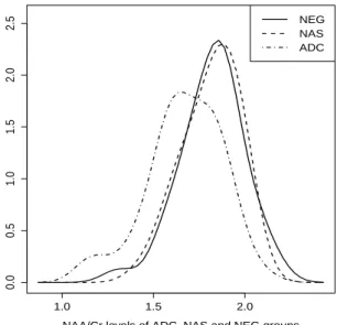
patients (Nakas et al., 2010; Chang et al., 2004). The NAA/Cr levels were available on 137 patients, of whom 61 were HIV-positive subjects with AIDS dementia complex ADC, 39 were HIV-positive non-symptomatic subjects NAS, and 37 were HIV-negative individuals NEG. The NAA/Cr levels are anticipated to be lowest among the ADC group and highest among the NEG group, with the NAS group being intermediate to the other two. This can be expressed as ADC < NAS < NEG (Chang et al., 2004), we refer to these groups as X,

Y and Z, respectively. Nakas et al. (2010) used this dataset to illustrate the generalized Youden index for thresholds selection in three-class classification problems. The empirical Youden index is maximised (equals to 1.434) at the threshold valuesc1 = 1.83 andc2 = 1.99.

We use this data set to illustrate the three methods presented in Sections 3, 4 and 5, namely 3-NPI, 3-NPI-Y and NPI-PW.

Figure 1 presents the probability density estimation of NAA/Cr levels for ADC, NAS and NEG, where a noticeable overlap between the three groups can be observed, in particular between the NAS and NEG groups. We may not be surprised if we found latter that the diagnostic test may struggle to distinguish between the later two groups, which leaves us with the question whether or not we should combine the latter two groups together and run the analysis again to achieve a better diagnostic accuracy, we will discuss this at the end of this example. As it is irrelevant howc1 andc2 are chosen within the respective intervals, the

reported values of c1 and c2 in this example are set be equal to the lower-end point of the

respective intervals plus 0.0005. One can also, for example, setc1 andc2 to be the mid-points

of these respective intervals, which we do in the simulations reported in Section 8, where it actually can have a small difference due to the explicit study of predictive performance on simulated future individuals.

1.0 1.5 2.0 0.0 0.5 1.0 1.5 2.0 2.5

NAA/Cr levels of ADC, NAS and NEG groups NEG NAS ADC

Figure 1: Density estimation of NAA/Cr levels for ADC, NAS and NEG

(16)

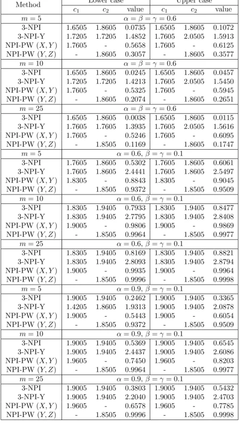
methods along with their corresponding lower and upper probabilities and for different values ofm. We have also considered three different scenarios ofα,β andγ. We notice that when α = β = γ = 0.6, all the methods provide the same optimal threshold values (c1, c2)

regardless of the m value, of course the corresponding lower and upper probabilities are different. For the scenario where α = 0.6 and β =γ = 0.1, that is we put less emphasis on the number of correctly classified future observations from groupsY andZ and more on the number of correctly classified future observations from groupX, we notice that all the lower and upper probabilities are of course greater than for the case whereα =β =γ = 0.6 and obviously we have different values of the optimal thresholds (c1, c2). For the scenario where

α = 0.9 and β =γ = 0.1, that is we are requesting even more emphasis on the number of correctly classified future observations from group X, the lower and upper probabilities are substantially smaller except for the NPI-PW (Y, Z) where they are obviously constant (as

(17)

Method Lower case Upper case c1 c2 value c1 c2 value m= 5 α=β =γ= 0.6 3-NPI 1.6505 1.8605 0.0735 1.6505 1.8605 0.1072 3-NPI-Y 1.7205 1.7205 1.4852 1.7605 2.0505 1.5913 NPI-PW (X, Y) 1.7605 - 0.5658 1.7605 - 0.6125 NPI-PW (Y, Z) - 1.8605 0.3057 - 1.8605 0.3577 m= 10 α=β =γ= 0.6 3-NPI 1.6505 1.8605 0.0245 1.6505 1.8605 0.0457 3-NPI-Y 1.7205 1.7205 1.4213 1.7605 2.0505 1.5450 NPI-PW (X, Y) 1.7605 - 0.5325 1.7605 - 0.5945 NPI-PW (Y, Z) - 1.8605 0.2074 - 1.8605 0.2651 m= 25 α=β =γ= 0.6 3-NPI 1.6505 1.8605 0.0038 1.6505 1.8605 0.0115 3-NPI-Y 1.7605 1.7605 1.3935 1.7605 2.0505 1.5616 NPI-PW (X, Y) 1.7605 - 0.5246 1.7605 - 0.6095 NPI-PW (Y, Z) - 1.8505 0.1169 - 1.8605 0.1747 m= 5 α= 0.6,β=γ= 0.1 3-NPI 1.7605 1.8605 0.5302 1.7605 1.8605 0.6061 3-NPI-Y 1.7605 1.8605 2.4441 1.7605 1.8605 2.5497 NPI-PW (X, Y) 1.8305 - 0.8843 1.8305 - 0.9045 NPI-PW (Y, Z) - 1.8505 0.9372 - 1.8505 0.9509 m= 10 α= 0.6,β=γ= 0.1 3-NPI 1.8305 1.9405 0.7933 1.8305 1.9405 0.8477 3-NPI-Y 1.8305 1.9405 2.7795 1.8305 1.9405 2.8408 NPI-PW (X, Y) 1.9005 - 0.9806 1.9005 - 0.9869 NPI-PW (Y, Z) - 1.8505 0.9964 - 1.8505 0.9977 m= 25 α= 0.6,β=γ= 0.1 3-NPI 1.8305 1.9405 0.8169 1.8305 1.9405 0.8821 3-NPI-Y 1.8305 1.9405 2.8093 1.8305 1.9405 2.8794 NPI-PW (X, Y) 1.9005 - 0.9935 1.9005 - 0.9964 NPI-PW (Y, Z) - 1.8505 0.9996 - 1.8505 0.9998 m= 5 α= 0.9,β=γ= 0.1 3-NPI 1.9005 1.9405 0.2462 1.9005 1.9405 0.3365 3-NPI-Y 1.4205 1.8605 1.9313 1.9005 1.9405 2.0878 NPI-PW (X, Y) 1.9005 - 0.5443 1.9005 - 0.6054 NPI-PW (Y, Z) - 1.8505 0.9372 - 1.8505 0.9509 m= 10 α= 0.9,β=γ= 0.1 3-NPI 1.9005 1.9405 0.5369 1.9005 1.9405 0.6545 3-NPI-Y 1.9005 1.9405 2.4437 1.9005 1.9405 2.6086 NPI-PW (X, Y) 1.9605 - 0.7450 1.9605 - 0.8203 NPI-PW (Y, Z) - 1.8505 0.9964 - 1.8505 0.9977 m= 25 α= 0.9,β=γ= 0.1 3-NPI 1.9005 1.9405 0.3803 1.9005 1.9405 0.5432 3-NPI-Y 1.9005 1.9405 2.2040 1.9005 1.9405 2.4703 NPI-PW (X, Y) 1.9605 - 0.6578 1.9605 - 0.7785 NPI-PW (Y, Z) - 1.8505 0.9996 - 1.8505 0.9998

Table 1: Optimal thresholds (c1, c2) using NPI-based methods

(18)

often tries to squeeze one of the groups in order to maximise the corresponding lower and upper probabilities (as it is based on summing up the individual probabilities rather than taking the product) while the 3-NPI method actually tries to balance between the groups (of course given that we choose α =β = γ) in order to find the optimal thresholds c1 and

c2. To illustrate this further, we have calculated the individual probabilities, the optimal

thresholds and the corresponding lower and upper probabilities of both methods and they are presented in Table 2. As we can see from this table, the 3-NPI-Y method squeezes group Y in order to obtain the optimal thresholds that maximise the lower probability in Equation (35), and thus focuses on maximising the number of correctly classified future observations from groups X and Z. In addition, the 3-NPI-Y method squeezes group Z

in order to obtain the optimal thresholds that maximise the upper probability in Equation (36), and thus focuses on maximising the number of correctly classified future observations from groups X and Y. On the other hand, the 3-NPI method tries to balance between the three groups in order to obtain the optimal thresholds that maximise both the lower and upper probabilities, but we also notice a slightly smaller value for the Y group in the lower probability case and a slightly higher value for theZ group for the upper probability case, but both values are still close to the values of the other groups.

cL1 cL2 P(C(X−∞,c1)≥αmx) P(C Y (c1,c2)≥βmy) P(C Z (c2,∞)≥γmz) 3-NPI-L 3-NPI-Y-L 1.6505 1.8605 0.4415 0.3676 0.4531 0.0735 − 1.7205 1.7205 0.6161 0.0000 0.8691 − 1.4852 cU1 cU2 P(C(X−∞,c1)≥αmx) P(C Y (c1,c2)≥βmy) P(C Z (c2,∞)≥γmz) 3-NPI-U 3-NPI-Y-U 1.6505 1.8605 0.4707 0.4553 0.5000 0.1072 − 1.7605 2.0505 0.7747 0.7907 0.0259 − 1.5913

Table 2: Comparison of 3-NPI and 3-NPI-Y methods, form= 5 andα=β =γ= 0.6, where (cL

1, cL2) and

(cU

1, cU2) are the corresponding thresholds of the lower and upper probabilities, respectively.

Method Lower case Upper case

c value c value α=β = 0.6,m= 5 2-NPI 1.7605 0.5688 1.7605 0.6024 2-NPI-Y 1.7605 1.5084 1.7605 1.5523 α=β = 0.6,m= 10 2-NPI 1.7605 0.5379 1.7605 0.5831 2-NPI-Y 1.7605 1.4668 1.7605 1.5272 α=β = 0.6,m= 25 2-NPI 1.7605 0.5364 1.7605 0.6002 2-NPI-Y 1.7605 1.4650 1.7605 1.5495

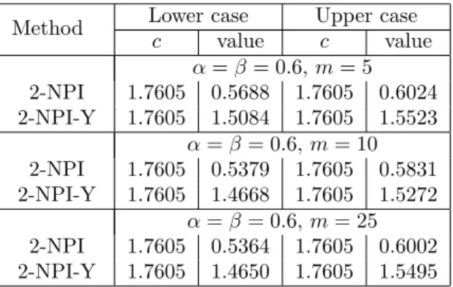
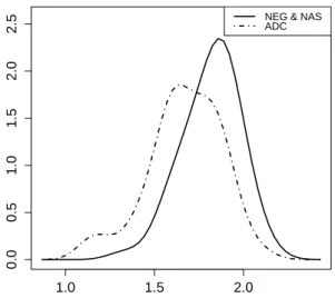
Table 3: Selecting the optimal thresholdcusing the NPI-based methods, when NAS and NEG are combined We notice, from Table 1, that when α = β = γ = 0.6, the lower and upper NPI-PW method based on groupsY andZ are much lower than those based on groupsX and Y, this is due to the fact that groups Y and Z overlap more than groups X and Y. If we combine

(19)

1.0 1.5 2.0 0.0 0.5 1.0 1.5 2.0 2.5

NEG & NAS ADC

Figure 2: Density estimation of NAA/Cr levels for ADC and (NAS, NEG) combined

the groupsY and Z together, as shown in Figure 2, and we run the analysis again, then the remaining NPI-based methods, 2-NPI and 2-NPI-Y, are presented in Table 3. As we can see from this table, all NPI-based methods give the same optimal threshold value atc= 1.7605 regardless of the value of m, this can happen but is not necessarily always the case. The empirical Liu’s index (2-EL) is equal to 0.4314 at the same threshold value as the NPI-based methods (atc= 1.7605) while the empirical Youden index (2-EY), which is equal to 0.3371, gives a different threshold value at c = 1.6605. We can also see by comparing the values of NPI-PW (X, Y) in Table 2 with the values of 2-NPI in Table 3 that we now have less imprecision (the difference between the upper and lower probabilities) when groups Y and

Z are combined.

8. Simulation

In order to study the performance of the methods presented in this paper, a simulation study was conducted for the two- and three-groups scenarios. We have considered two main cases, in which the data are simulated from the following normal distributions:

Case A: X ∼N(0,22_),_Y _∼_N₍₁_,₂2_{), and}_Z _∼_N₍₃_,₂2_).

Case B: X ∼N(0,12), Y ∼N(1,12), and Z ∼N(3,12).

The data set from group Z is only used when the three-groups scenario is considered, and due to the large variance in Case A, the groups in that case overlap more than in Case B. The mx, my and mz future observations will be simulated from the same underlying

(20)

observations will be used to find the optimal thresholds (cin the two-groups scenario, and

c1 and c2 in the three-groups scenario) according to these methods and for specific values

of (α, β, γ) when applicable, where the optimal threshold values are set to the midpoint within the search intervals. Then the simulated future observations (future test results) are compared with the optimal thresholds to obtain the number of correctly classified observa-tions per group. That is, for the two-groups scenario, the number of future observaobserva-tions out of mx (my) with the simulated test results are less or equal to (greater than) c are

obtained. Similarly for the three-groups scenario, the number of correctly classified future observations is the number of future observations out of mx with the simulated test results

less than or equal toc1, the number of future observations out ofmy with the simulated test

results in (c1, c2], and the number of future observations out of mz with the simulated test

results greater thanc2. The number of correctly classified future observations in all

simula-tions from groups X, Y and Z are denoted by SX jx, S

Y

jy and S

Z

jz, where jx ∈ {0,1, . . . , mx}, jy ∈ {0,1, . . . , my} and jz ∈ {0,1, . . . , mz}, respectively. Bar plots have been used to

sum-marise these numbers from all methods as shown later in this section. We have studied the prediction performance of all methods in terms of the number of correctly classified future observations that are achieved using the desired criteria, that is when the number of cor-rectly classified future observations from group X, Y, and Z exceed αmx, βmy and γmz,

respectively. Let us denote by ”+” when the desired criteria is achieved and ”-” otherwise. Throughout this section we assume that nx =ny =nz =n and mx =my =mz =m, thus

jx =jy =jz =j and j ∈ {0,1, . . . , m}.

For the two-group scenario, we run the simulation for n = 10 and m = 5,30, while for the three-groups scenario we have considered n = 20 and m= 3,10. For both scenarios we have chosen different values of α, β and γ, obviously these selected values have no impact on Youden’s index and Liu’s index in terms of selecting the optimal thresholds, however for the sake of the comparison we have involved α, β and γ when we compared the prediction performance of these two methods with the proposed methods, that is we have considered the same desired criteria, that is the number of future observations that are correctly classified from groups X, Y and Z are at least αm, βm and γm, respectively. The results in this section are based on 10,000 simulations per case per setting.

8.1. Two-groups scenario

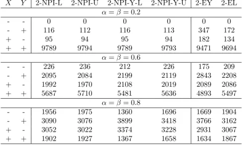
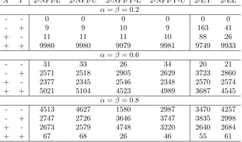
The prediction performance results for Case A are given in Tables 4 and 5 form= 5 and

m = 30, respectively, and in Tables 6 and 7 for Case B. We have studied the performance for n = 10 and α = β = 0.2,0.6,0.8 for the NPI-based methods (2-NPI and 2-NPI-Y) and the empirical estimates of Youden’s index and Liu’s index (2-EY and 2-EL).

Considering Table 4, for example, where ”+ +” indicates that the desired criteria is achieved for both groups while ”− −” indicates that the desired criteria is not achieved for both groups. For example, for 2-NPI-Y-U and α = β = 0.2 the desired criteria has been achieved for both groups 9886 out of 10,000 simulations, that is at least 6 future observations (αm= 0.2×30 andβm= 0.2×30) are correctly classified from the disease and non-disease groups. On the other hand, only 62 out of 10,000 simulations in which the desired criteria

(21)

is achieved (6 or more out of 30 are correctly classified) from the non-disease group (group

X) and the desired criteria is not achieved for the disease group (group Y).

From Tables 4-7, the 2-NPI (2-NPI-L and 2-NPI-U) method clearly outperforms all the other methods and for all the settings that have been considered. While for small values of α and β it appears that the 2-NPI and 2-NPI-Y perform similarly, the 2-NPI-Y method performs poorly for larger values of α and β . One possible explanation is that the 2-NPI-Y method is based on the sum of the probabilities of correct classification rather than the product, which seems not ideal if one tries to achieve higher proportions of those who are correctly classified. Yet for small values of α and β, as we have mentioned earlier the 2-NPI-Y method performs equally well as the 2-NPI method.

Interestingly, the Liu’s index (2-EL) is the closest in terms of performance to the 2-NPI method over all settings, apart of course of the 2-NPI-Y method inconsistent performance that has been discussed above. It is not surprising that Liu’s index performs better than Youden’s index, as we have already discussed that summing up the probabilities of correct classification may not be ideal when considering the prediction performance. We also notice that Youden’s index is actually performing better than the 2-NPI-Y method for larger values of α and β, this is interesting as one may think that the 2-NPI-Y method should have a similar performance as Youden’s index or even better (considering its predictive nature), however, we should not forget that α and β have not been used to obtain the optimal threshold using Youden’s index, while these α and β are involved in finding the optimal threshold using the 2-NPI-Y method.

In addition, all methods perform poorly with the increase of α and β as the criteria become harder to achieve. On the other hand, all methods also tend to perform poorly when m increases, except for smaller values of α and β. Finally, and not surprisingly, all methods perform much better in Case B than in Case A, as the groups in Case B are more separated than in Case A.

X Y 2-NPI-L 2-NPI-U 2-NPI-Y-L 2-NPI-Y-U 2-EY 2-EL

α=β= 0.2 - - 0 0 0 0 0 0 - + 301 293 301 294 890 424 + - 259 249 259 249 620 356 + + 9440 9458 9440 9457 8490 9220 α=β= 0.6 - - 793 795 664 747 540 741 - + 2869 2854 3372 3040 3844 3039 + - 2795 2787 2937 2882 3034 2911 + + 3543 3564 3027 3331 2582 3309 α=β= 0.8 - - 3556 3575 1684 2447 2734 3455 - + 2885 2874 4686 3902 3749 2999 + - 2797 2779 3325 3149 2962 2815 + + 762 772 305 502 555 731

(22)

X Y 2-NPI-L 2-NPI-U 2-NPI-Y-L 2-NPI-Y-U 2-EY 2-EL α=β= 0.2 - - 0 0 0 0 0 0 - + 52 50 54 52 752 185 + - 63 65 62 62 542 172 + + 9885 9885 9884 9886 8706 9643 α=β= 0.6 - - 867 890 586 797 488 751 - + 3943 3922 4753 4162 4905 4203 + - 3624 3595 3606 3617 3748 3696 + + 1566 1593 1055 1424 859 1350 α=β= 0.8 - - 7043 7186 1461 2701 5003 6746 - + 1495 1447 3327 4450 2899 1753 + - 1460 1365 5212 2848 2097 1499 + + 2 2 0 1 1 2

Table 5: Case A:n= 10 andm= 30

X Y 2-NPI-L 2-NPI-U 2-NPI-Y-L 2-NPI-Y-U 2-EY 2-EL

α=β= 0.2 - - 0 0 0 0 0 0 - + 116 112 116 113 347 172 + - 95 94 95 94 182 134 + + 9789 9794 9789 9793 9471 9694 α=β= 0.6 - - 226 236 212 226 175 209 - + 2095 2084 2199 2119 2843 2208 + - 1992 1970 2108 2019 2089 2086 + + 5687 5710 5481 5636 4893 5497 α=β= 0.8 - - 1956 1975 1360 1696 1669 1904 - + 3090 3076 3899 3418 3766 3162 + - 3052 3022 3374 3228 2931 3067 + + 1902 1927 1367 1658 1634 1867

(23)

X Y 2-NPI-L 2-NPI-U 2-NPI-Y-L 2-NPI-Y-U 2-EY 2-EL α=β= 0.2 - - 0 0 0 0 0 0 - + 9 9 10 9 163 41 + - 11 11 11 10 88 26 + + 9980 9980 9979 9981 9749 9933 α=β= 0.6 - - 31 33 26 34 20 21 - + 2571 2518 2905 2629 3723 2860 + - 2377 2345 2546 2348 2570 2574 + + 5021 5104 4523 4989 3687 4545 α=β= 0.8 - - 4513 4627 1580 2987 3470 4257 - + 2747 2726 3646 3747 3835 2998 + - 2673 2579 4748 3220 2640 2684 + + 67 68 26 46 55 61

Table 7: Case B:n= 10 andm= 30

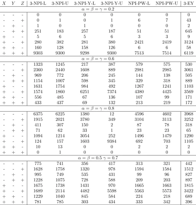
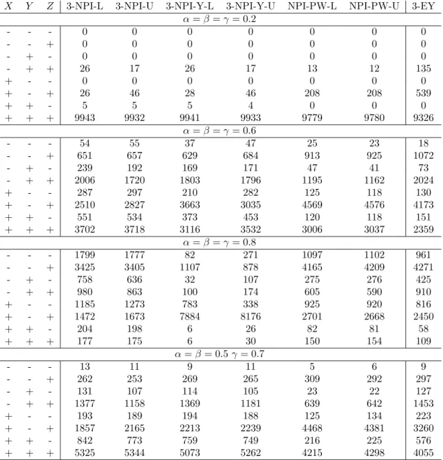
8.2. Three-groups scenario

In this section, we consider the three-groups scenario, where we study the predictive performance of all methods for the two cases mentioned above. The prediction performance results for Case A are given in Tables 8 and 9 for m = 10 andm = 30, respectively, and in Tables 10 and 11 for Case B. We have studied the performance for n = 20, α = β = γ ∈ {0.2,0.6,0.8}, and when α =β = 0.5, γ = 0.7 for the NPI-based methods (3-NPI, 3-NPI-Y and NPI-PW) and the empirical estimates of Youden’s index (3-EY).

From these tables, we observed similar behaviour as in the two-groups scenario. Again the 3-NPI-Y method performs equally well as the 3-NPI method, however, the performance of the 3-NPI-Y method is worse when α, β and γ are larger. Interestingly, the NPI-PW method has better performance than the empirical Youden’s index (3-EY) whenα=β =γ. Again Youden’s index performs better than the 3-NPI-Y method for larger values of α, β

andγ due to the same reasoning as discussed for the two-groups scenario in Section 8.1. We also notice that for larger values of α, β and γ, the 3-NPI-Y tends to squeeze the middle group Y substantially, while Youden’s index tends to squeeze groups Y in some occasions or even squeeze all groups in one group (group Z in this case). While the NPI-PW method squeezes groupY on some occasions and squeezes all the groups in one groupZ in others, it still provides large numbers of correctly classified future observations. Figures 3-6 show the distributions of the numbers of future observations out ofm in all 10,000 simulations, that are correctly classified for each group, the squeezing behaviour of the 3-NPI-Y, NPI-PW and 3EY methods is clearly shown.

(24)

X Y Z 3-NPI-L 3-NPI-U 3-NPI-Y-L 3-NPI-Y-U NPI-PW-L NPI-PW-U 3-EY α=β=γ= 0.2 - - - 0 0 0 0 0 0 0 - - + 0 1 0 1 6 7 43 - + - 1 0 1 0 0 0 2 - + + 251 183 257 187 51 51 645 + - - 5 6 5 6 3 3 9 + - + 280 382 281 380 2421 2419 3124 + + - 160 128 158 126 6 6 58 + + + 9303 9300 9298 9300 7513 7514 6119 α=β=γ= 0.6 - - - 1323 1245 217 387 579 575 530 - - + 2360 2440 1608 889 2981 2985 3061 - + - 969 772 206 245 144 138 505 - + + 1154 1007 598 345 329 318 889 + - - 1631 1754 984 492 1267 1241 1103 + - + 1574 1860 6251 7374 4380 4425 3569 + + - 556 485 67 136 107 99 171 + + + 433 437 69 132 213 219 172 α=β=γ= 0.8 - - - 6375 6225 1380 12 4596 4602 3968 - - + 1915 2021 3780 349 3104 3113 3252 - + - 411 307 150 2 87 78 318 - + + 71 62 33 1 23 23 65 + - - 1094 1214 3054 252 1496 1479 1290 + - + 124 157 1603 9384 692 703 1105 + + - 10 13 0 0 2 2 2 + + + 0 1 0 0 0 0 0 α=β= 0.5γ= 0.7 - - - 775 741 356 417 313 321 442 - - + 1628 1758 1320 978 1594 1584 1512 - + - 995 749 535 431 99 96 827 - + + 1228 1075 728 588 209 203 897 + - - 1675 1738 1431 970 1665 1663 1815 + - + 1689 2114 4482 5598 5563 5573 3422 + + - 1229 1040 845 584 224 218 689 + + + 781 785 303 434 333 342 396

(25)

(26)

(27)

Table 11: Case B m= 30 andn= 20

From Figures 3-6, we can see that for larger values of α = β = γ, all methods struggle to meet the required criteria, especially in Case A where the groups have more overlap. We also notice that the number of correctly classified future observations from group Z is much larger than from groups X and Y, as group Z is more separated in comparison to the other two groups. In addition, selecting the values of α, β and γ will have impact on the number of correctly classified future observations, for example, the number of correctly classified future observations when α = β = γ = 0.6 is lower than when α = β = 0.5 and

γ = 0.7 for both cases. From Tables 8 to 11, we can see that when α = β = γ = 0.6 and

α = β = γ = 0.8 all the methods perform better for small value of m than for larger m, while for α = β = γ = 0.2 all the methods perform better for large m than for small m.

(28)

Obviously, all methods perform much better in Case B than in Case A, as the groups in Case B are more separated than in Case A.

(29)

0 2000 4000 6000 0 1 2 3 4 5 6 7 8 9 10 j S_jX Method 3−NPI−L 3−NPI−U 3−NPI−Y−L 3−NPI−Y−U NPI−PW−L NPI−PW−U 3−EY 0 2000 4000 6000 0 1 2 3 4 5 6 7 8 9 10 j S_jY Method 3−NPI−L 3−NPI−U 3−NPI−Y−L 3−NPI−Y−U NPI−PW−L NPI−PW−U 3−EY 0 2000 4000 6000 0 1 2 3 4 5 6 7 8 9 10 j S_jZ Method 3−NPI−L 3−NPI−U 3−NPI−Y−L 3−NPI−Y−U NPI−PW−L NPI−PW−U 3−EY

(30)

0 2500 5000 7500 10000 0 1 2 3 4 5 6 7 8 9 10 j S_jX Method 3−NPI−L 3−NPI−U 3−NPI−Y−L 3−NPI−Y−U NPI−PW−L NPI−PW−U 3−EY 0 2500 5000 7500 10000 0 1 2 3 4 5 6 7 8 9 10 j S_jY Method 3−NPI−L 3−NPI−U 3−NPI−Y−L 3−NPI−Y−U NPI−PW−L NPI−PW−U 3−EY 0 2500 5000 7500 10000 0 1 2 3 4 5 6 7 8 9 10 j S_jZ Method 3−NPI−L 3−NPI−U 3−NPI−Y−L 3−NPI−Y−U NPI−PW−L NPI−PW−U 3−EY

(31)

(32)

(33)

9. Concluding remarks

This paper considered the choice of thresholds for diagnostic tests, with two or three groups, explicitly as a predictive problem instead of the classical approach based on estima-tion. We considered m individuals in each group for who the thresholds would be applied, and criteria in terms of the proportions of successful diagnoses. Nonparametric predictive inference was applied to derive the optimal thresholds, which were shown to depend on the target success proportions and also on the value of m. Our method provides a gen-eral theoretic investigation into setting diagnostic thresholds from a predictive perspective, for mx future healthy people and my future patients, where we mostly restrict analysis to

mx = my = m. Of course, in practice one would not know a specific value of m but the

main idea is to investigate how the optimal threshold can vary for different values of m. If, however, there is a scenario with specific numbers mx and my of interest, then the method

can be straightforwardly applied. The methods were illustrated by an example using data from the literature, and the performance was evaluated through simulation studies. These revealed that, in case of three group scenarios for which the classical Youden’s index ap-proach is used, one of the groups may have very poor predictive performance, this is avoided by the methods presented in this paper.

NPI is a statistical method with strong frequentist properties, in line with the notion of exact calibration as introduced by Lawless and Fredette (2005). Contrary to most classical frequentist statistics methods, NPI does not consider data as resulting from an assumed sam-pling method related to an assumed population. Instead, by focusing on future observations, the variation is in the possible orderings of the data observations and future observations, so the randomness is explicitly in the prediction. In absence of knowledge about the un-derling population distribution, this is an alternative approach. If one had such additional knowledge, then one could attempt to combine NPI with aspects of sample variation; this is an interesting topic for future research.

This line of work provides many questions and opportunities for future research. For example, one may wish to consider how one can set meaningful target proportions for the predictive inferences, or to develop similar approaches for different kinds of data, e.g. ordinal data. Another example would be instead of using the proposed method for selecting the optimal thresholds based on the sensitivity and specificity of the test, it may be attractive to use such a method to select the optimal thresholds based on positive and negative predictive values (PPV, NPV). To this end, one needs to consider carefully the events of interest for the NPI approach to PPV and NPV. If one measures multiple markers per patient, their optimal combination together with optimal selection of thresholds is of interest, while also taking dependence of such multivariate data into account provides interesting challenges, A further challenge is to develop such methods for data containing right-censored observations. Some of these topics require further development of NPI, including methods for multivariate data and for multiple future observations based on right-censored data. Generally, consid-ering such problems from a predictive perspective, in particular also how the number of future individuals considered might influence the optimal thresholds, provides interesting new insights which may also have substantial practical relevance.

(34)

Acknowledgement

We are grateful to Dr. Christos Nakas for providing the data set used in the example. The authors would like to thank an anonymous reviewer for supporting this work and for valuable comments that led to improved presentation.

References

Alabdulhadi, M., 2018. Nonparametric predictive inference for diagnostic test thresholds. Ph.D. thesis, Durham University, Durham, UK.

Alqifari, H., 2017. Nonparametric predictive inference for future order statistics. Ph.D. thesis, Durham University, Durham, UK.

Augustin, T., Coolen, F. P., 2004. Nonparametric predictive inference and interval probability. Journal of Statistical Planning and Inference 124 (2), 251–272.

Chang, L., Lee, P., Yiannoutsos, C. T., Ernst, T., Marra, C., Richards, T., Kolson, D., Schifitto, G., Jarvik, J., Miller, E., et al., 2004. A multicenter in vivo proton-mrs study of hiv-associated dementia and its relationship to age. Neuroimage 23 (4), 1336–1347.

Coolen, F. P., 2006. On nonparametric predictive inference and objective bayesianism. Journal of Logic, Language and Information 15 (1-2), 21–47.

Coolen, F. P., 2011a. Nonparametric predictive inference. In: International encyclopedia of statistical science. Springer, pp. 968–970.

Coolen, F. P., Coolen-Maturi, T., Alqifari, H. N., 2017. Nonparametric predictive inference for future order statistics. Communications in Statistics: Theory and Methods, to appear.

Coolen, F. P., Maturi, T. A., 2010. Nonparametric predictive inference for order statistics of future obser-vations. In: Combining Soft Computing and Statistical Methods in Data Analysis. Springer, pp. 97–104. Coolen, F. P. A., 2011b. Nonparametric predictive inference. In: Lovric, M. (Ed.), International Encyclopedia

of Statistical Science. Springer, pp. 968–970.

Coolen-Maturi, T., 2017a. Predictive inference for best linear combination of biomarkers subject to limits of detection. Statistics in Medicine 36 (18), 2844–2874.

Coolen-Maturi, T., 2017b. Three-group roc analysis predictive analysis for ordinal outcomes. Communica-tions in Statistics: Theory and Methods 46 (19), 9476–9493.

Coolen-Maturi, T., Coolen-Schrijner, P., Coolen, F. P., 2012a. Nonparametric predictive inference for binary diagnostic tests. Journal of Statistical Theory and Practice 6 (4), 665–680.

Coolen-Maturi, T., Coolen-Schrijner, P., Coolen, F. P., 2012b. Nonparametric predictive inference for diag-nostic accuracy. Journal of Statistical Planning and Inference 142 (5), 1141–1150.

Coolen-Maturi, T., Elkhafifi, F. F., Coolen, F. P., 2014. Three-group roc analysis: A nonparametric predic-tive approach. Computational Statistics & Data Analysis 78, 69–81.

Elkhafifi, F. F., Coolen, F. P., 2012. Nonparametric predictive inference for accuracy of ordinal diagnostic tests. Journal of Statistical Theory and Practice 6 (4), 681–697.

Finetti, B. d., 1974. Theory of probability. a critical introductory treatment.

Fluss, R., Faraggi, D., Reiser, B., 2005. Estimation of the youden index and its associated cutoff point. Biometrical Journal 47 (4), 458–472.

Geisser, S., 1993. Predictive inference. Vol. 55. CRC Press.

Hand, D. J., 2009. Measuring classifier performance: a coherent alternative to the area under the roc curve. Machine learning 77 (1), 103–123.

Hill, B. M., 1968. Posterior distribution of percentiles: Bayes’ theorem for sampling from a population. Journal of the American Statistical Association 63 (322), 677–691.

Hill, B. M., 1988. De finettis theorem, induction, and a(n) or bayesian nonparametric predictive inference (with discussion). Bayesian statistics 3, 211–241.

Jund, J., Rabilloud, M., Wallon, M., Ecochard, R., 2005. Methods to estimate the optimal threshold for normally or log-normally distributed biological tests. Medical decision making 25 (4), 406–415.