A Machine Learning Approach to Credit Allocation
by
Domonkos F. Vamossy
B.A. in Mathematical Economics and Mathematics, Whitworth University, 2015
M.A. in Economics, University of Pittsburgh, 2017
Submitted to the Graduate Faculty of
the Dietrich School of Arts and Sciences in partial fulfillment
of the requirements for the degree of
Doctor of Philosophy
UNIVERSITY OF PITTSBURGH
DIETRICH SCHOOL OF ARTS AND SCIENCES
This dissertation was presented by
Domonkos F. Vamossy
It was defended on July 20, 2020 and approved by
Stefania Albanesi, Professor of Economics, University of Pittsburgh Daniel Berkowitz, Professor of Economics, University of Pittsburgh Douglas Hanley, Assistant Professor of Economics, University of Pittsburgh
Sera Linardi, Associate Professor of Economics, University of Pittsburgh Dokyun Lee, Assistant Professor of Business Analytics, Carnegie Mellon University Dissertation Director: Stefania Albanesi, Professor of Economics, University of Pittsburgh
Copyright cby Domonkos F. Vamossy 2020
A Machine Learning Approach to Credit Allocation
Domonkos F. Vamossy, PhD University of Pittsburgh, 2020
This dissertation seeks to understand the shortcomings of contemporaneous credit allo-cation, with a specific focus on exploring how an improved statistical technology impacts the credit access of societally important groups. First, this dissertation investigates a variety of limitations of conventional credit scoring models, specifically their tendency to misclassify borrowers by default risk, especially for relatively risky, young, and low income borrowers. Second, this dissertation shows that an improved statistical technology need not to lead to worse outcomes for disadvantaged groups. In fact, the credit access for borrowers belong-ing to such groups can be improved, while providbelong-ing more accurate credit risk assessment. Last, this dissertation documents modern-day disparities in debt collection judgments across white and black neighborhoods. Taken together, this dissertation provides valuable insights for the design of policies targeted at reducing consumer default and alleviating its burden on borrowers and lenders and across societally important groups, as well as macroprudential regulation.
Table of Contents
Preface . . . xiv
1.0 Predicting Consumer Default: A Deep Learning Approach . . . 1
1.1 Introduction . . . 1
1.2 Data . . . 8
1.3 Patterns in Consumer Default . . . 8
1.3.1 Default Transitions . . . 9
1.3.2 Non-linearities . . . 10
1.3.3 High Order Interactions . . . 11
1.4 Model . . . 12
1.4.1 Deep Neural Network . . . 13
1.4.2 eXtreme Gradient Boosting (XGBoost) . . . 14
1.4.3 Hybrid DNN-GBT Model . . . 14
1.4.4 Implementation . . . 15
1.5 Comparison with Credit Score . . . 15
1.5.1 Ranking . . . 16
1.5.2 Feature Attribution . . . 19
1.5.3 Vulnerable Populations . . . 20
1.5.4 Mortgage Default . . . 22
1.6 Applications . . . 23
1.6.1 Predicting Systemic Risk . . . 23
1.6.2 Value Added . . . 24
1.6.2.1 Lenders . . . 24
1.6.2.2 Borrowers . . . 25
1.7 Conclusion . . . 27
2.1 Introduction . . . 42
2.2 Data . . . 46
2.2.1 Generating Groups . . . 47
2.2.2 On Race Proxies . . . 47
2.3 Motivating Evidence . . . 48
2.4 Constrained Machine Learning: A Conceptual Framework . . . 50
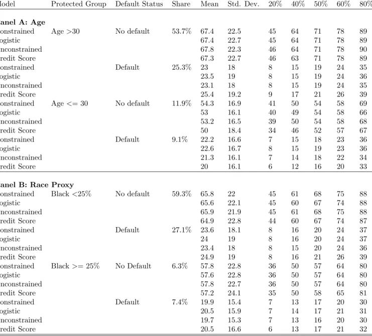
2.5 Fairness Constraints . . . 51 2.5.1 Descriptive Statistics . . . 51 2.5.2 Age . . . 52 2.5.3 Race Proxy . . . 52 2.6 Applications . . . 53 2.6.1 Access to Credit . . . 53 2.6.2 Counterfactual Rankings . . . 53 2.6.3 Value Added . . . 54 2.6.3.1 Lenders . . . 54 2.7 Conclusion . . . 55
2.8 Figures and Tables . . . 56
3.0 Racial Disparities in Debt Collection . . . 63
3.1 Introduction . . . 63
3.2 Background Information . . . 67
3.2.1 Debt Collection Litigation Process . . . 67
3.2.2 Laws Regulating Debt Collection . . . 68
3.3 Data . . . 69 3.3.1 Race Proxies . . . 71 3.3.2 Sample Selection . . . 72 3.4 Empirical Strategy . . . 73 3.4.1 Summary Statistics . . . 74 3.4.2 Empirical Specification . . . 75 3.5 Results . . . 76
3.5.2 Debt Characteristics . . . 78
3.5.3 Lending Institutions . . . 79
3.5.4 Attorney Representation and Judgment Type . . . 79
3.5.5 Non-linearities & Higher Order Interactions . . . 81
3.5.5.1 Explanatory Power of Variables . . . 81
3.5.6 Differences in Plaintiff Type . . . 82
3.6 Robustness Checks . . . 83
3.6.1 Race Proxies . . . 83
3.6.1.1 Other Races . . . 84
3.6.2 Selection on Unobservables . . . 84
3.6.3 Alternative Credit Score . . . 85
3.6.4 Evolution of Disparity . . . 85
3.6.5 Alternative Data Sources . . . 86
3.7 Conclusion . . . 86
3.8 Figures and Tables . . . 88
Appendix A. Predicting Consumer Default: A Deep Learning Approach . 100 A.1 Performance Metrics . . . 100
A.2 Data Pre-Processing . . . 101
A.2.1 Sample Restrictions . . . 101
A.2.2 Feature Scaling . . . 101
A.2.3 Train-Test Split . . . 101
A.2.4 Features . . . 102
A.2.5 Feature Groups . . . 102
A.3 Machine Learning Models . . . 102
A.3.1 Deep Neural Network (DNN) . . . 102
A.3.2 Decision Tree Models . . . 104
A.3.2.1 CART . . . 105
A.3.2.2 Gradient Boosted Trees (GBT) . . . 105
A.4.2 DNN Optimization Algorithm . . . 107
A.4.3 GBT Algorithm . . . 108
A.4.4 Regularization . . . 109
A.4.5 Feature Selection . . . 109
A.4.6 Hyperparameter Selection . . . 110
A.4.7 Weighting . . . 111
A.4.8 Implementation . . . 111
A.5 Classifier Performance . . . 112
A.6 Model Interpretation . . . 116
A.6.1 Explanatory Power of Variables . . . 116
A.6.2 Economic Significance of Variables . . . 118
A.6.3 Temporal Determinants of Default . . . 120
A.7 Model Comparisons . . . 121
A.7.1 Hidden Layers . . . 121
A.7.2 Alternative Models . . . 122
A.7.3 Expanded Training Data . . . 123
A.8 Monotonicity Constraints . . . 123
A.9 Comparison with Credit Scores . . . 124
A.10 Additional Figures and Tables . . . 126
Appendix B. Towards Fair Credit Allocation . . . 149
B.1 Features . . . 149 B.2 Classifier Performance . . . 149 B.2.1 Unconstrained Models . . . 150 B.2.2 Constrained Models . . . 150 B.3 Model Interpretation . . . 150 B.4 Additional Tables . . . 152
Appendix C. Racial Disparities in Debt Collection . . . 158
C.1 Judgment Data . . . 158
C.2 BISG Algorithm . . . 159
C.3 Expanded Sample . . . 160 C.4 Additional Figures and Tables . . . 161
List of Tables
1 Descriptive Statistics . . . 34
2 Default Transitions . . . 34
3 Borrower Rankings . . . 35
4 Credit Risk Differences . . . 36
5 Feature Attribution Differences . . . 37
6 Descriptive Statistics (Vulnerable Populations) . . . 37
7 Vulnerable Populations . . . 38
8 Mortgage Default Categories . . . 39
9 Descriptive Statistics (Mortgage Default) . . . 39
10 Comparison across Mortgage Default Types . . . 40
11 Cost of Credit Risk Misclassification . . . 41
12 The Unequal Effects of an Improved Statistical Technology . . . 57
13 Summary Statistics . . . 58
14 Constraining by Age . . . 59
15 Constraining by Race . . . 60
16 Access to Credit across Protected Groups . . . 61
17 Counterfactual Rankings . . . 62
18 Summary Statistics . . . 94
19 Judgments, Income, and Credit Scores . . . 95
20 Judgments and Debt Portfolios . . . 95
21 Judgments and Lending Institutions . . . 96
22 Attorney Representation and Judgment Type . . . 97
23 Judgments by Plaintiff Type . . . 97
24 Judgments and Other Measures of Racial Composition . . . 98
25 Judgments and Other Demographic Groups . . . 99
27 Model Inputs . . . 132
28 Summary Statistics . . . 133
29 Feature Groups . . . 134
30 Hyperparameters for Machine Learning Models: Out-of-sample Exercise . . . 134
31 Weighting Schemes and Loss . . . 135
32 1 Quarter Ahead Predictions, Full Sample– Hybrid DNN-GBT . . . 136
33 1 Quarter Ahead Predictions, Current– Hybrid DNN-GBT . . . 137
34 Performance Metrics using Hybrid DNN-GBT, Full Sample . . . 138
35 Performance Metrics using Hybrid DNN-GBT, Current . . . 139
36 Explanatory Power of Variables . . . 140
37 SHAP Values over Time . . . 141
38 Neural Networks Comparison: Loss & Accuracy . . . 142
39 Model Comparison: Out-of-Sample Loss . . . 143
40 Shap Values across Models . . . 144
41 Shap Values across Debt Categories . . . 144
42 Model Comparison: DNN vs. GBT, 1 Year . . . 145
43 Model Comparison: DNN vs. GBT, Full . . . 146
44 Constraining Model Behavior . . . 147
45 Distribution of Customers by Credit Score and Predicted Default . . . 148
46 Performance Metrics using Logistic Regression . . . 152
47 Performance Metrics using Unconstrained DNN . . . 153
48 Performance Metrics using Constrained DNN by Age . . . 154
49 Performance Metrics using Constrained DNN by Race . . . 155
50 SHAP Values: Unconstrained Models . . . 156
51 SHAP Values: Constrained Models . . . 157
52 Judgment Rates . . . 163
53 Judgments and an Alternative Credit Score . . . 164
54 Summary Statistics (NJ and IL Sample) . . . 165
57 Judgments, Income, and Credit Scores (Individual Judgment Data) . . . 167
58 Judgments and Debt Portfolios (Individual Judgment Data) . . . 167
59 Summary Statistics (Full Sample) . . . 168
60 Judgments, Income, and Credit Scores (Full Sample) . . . 169
61 Judgments and Other Measures of Racial Composition (Full Sample) . . . 170
62 Judgments and Other Demographic Groups (Full Sample) . . . 171
List of Figures
1 Outstanding Consumer Credit and Delinquency over Time . . . 28
2 Nonlinear Relation Between Default and Covariates . . . 29
3 Multidimensional Relation Between Default and Covariates . . . 30
4 Default Rates and Predicted Default Probability: Scatter Plot . . . 31
5 Default Rates and Predicted Default Probability: Polynomial Approximation . . 31
6 Differences in Creditworthiness by Age across and over Time . . . 32
7 Consumers with 90+ Days Delinquency: Predicted vs. Realized . . . 32
8 Value-Added of Machine Learning Forecasts . . . 33
9 Value-Added of Constrained Machine-Learning Forecasts . . . 56
10 Kernel Density Estimates of Selected Covariates . . . 89
11 Judgments and Demographic Composition . . . 90
12 Income, Credit Scores, and Judgment Rate . . . 91
13 GBT Feature Explanations . . . 92
14 Disparity over Time . . . 93
15 Two Layer Neural Network Example . . . 126
16 Confusion Matrix and Receiver Operating Characteristic (ROC) Curve . . . 127
17 SHAP Applied to Model Output . . . 128
18 Out-of-Sample ROC Curves for Various Models with Dropout . . . 128
19 Credit Score Histogram by Years . . . 129
20 Absolute Value of Rank Correlation with Realized Default Rate . . . 130
21 Propensity Score Distributions . . . 161
Preface
I am incredibly grateful to my advisor, Stefania Albanesi, for her constant guidance and encouragement. Her mentorship, collaboration, and the credit report data she provided, made this dissertation possible. I am also fortunate to have Dokyun Lee on my committee, whose class sparked my interest in exploring machine learning applications in economics, and whose help substantially improved my work. Sera Linardi is also someone I am extremely thankful for, her energy, enthusiasm and love of work set a great example for me. I would also like to thank Daniel Berkowitz and Douglas Hanley, along with the rest of the faculty members and administrators in the Economics Department at the University of Pittsburgh for their advice, support and assistance over the years. Special thanks to Osea Giuntella, Rania Gihleb, Georgia Spears, Brian Deutsch, Jessica LaVoice, Mallory Avery, Mark Azic, Lucy Wang, Lan Morrall, Max Myers, Tristan Cunha, and Viraj Mehta along with my amazing officemates and the rest of the graduate students in the Economics Department at the University of Pittsburgh for their friendship.
Finally, I would like to express my gratitude to my incredible family for their uncondi-tional love and support. Special thanks to my parents, my great uncle, Julius Varallyay, and my grandmother, who set me up on this journey roughly eight years ago. Last, I dedicate this work to my late grandfather, Ferenc V´amossy, who I inherited my middle name from, and who would have been thrilled to read this dissertation.
1.0 Predicting Consumer Default: A Deep Learning Approach
(joint with Stefania Albanesi) We develop a model to predict consumer default based on deep learning. We show that the model consistently outperforms standard credit scor-ing models, even though it uses the same data. Our model provides favorable credit risk assessment to young borrowers and is better at capturing mortgage default relative to stan-dard credit scoring models, while accurately tracking variations in systemic risk. We argue that these properties can provide valuable insights for the design of policies targeted at reducing consumer default and alleviating its burden on borrowers and lenders, as well as macroprudential regulation.
1.1 Introduction
The dramatic growth in household borrowing since the early 1980s has increased the macroeconomic impact of consumer default. Figure 1 displays total consumer credit balances in millions of 2018 USD and the delinquency rate on consumer loans starting in 1985. The delinquency rate mostly fluctuates between 3 and 4%, except at the height of the Great Recession when it reached a peak of over 5%, and in its aftermath when it dropped to a low of 2%. With the rise in consumer debt, variations in the delinquency rate have an ever larger impact on household and financial sector balances sheets. Understanding the determinants of consumer default and predicting its variation over time and across types of consumers can not only improve the allocation of credit, but also lead to important insights for the design of policies aimed at preventing consumer default or alleviating its effects on borrowers and lenders. They are also critical for macroprudential policies, as they can assist with the assessment of the impact of consumer credit on the fragility of the financial system. This paper proposes a novel approach to predicting consumer default based on deep learning. We rely on deep learning as this methodology is specifically designed for
predic-interaction among factors affecting the outcome of interest, for which standard regression approaches perform poorly. Our methodology uses the same information as standard credit scoring models, which are one of the most important factors in the allocation of consumer credit. We show that our model improves the accuracy of default predictions while increasing transparency and accountability. It is also able to track variations in systemic risk, and is able to identify the most important factors driving defaults and how they change over time. Finally, we show that adopting our model can accrue substantial savings to borrowers and lenders.
Credit scores constitute one of the most important factors in the allocation of consumer credit in the United States. They are proprietary measures designed to rank borrowers based on their probability of future default. Specifically, they target the probability of a 90 days past due delinquency in the next 24 months.1 Despite their ubiquitous use in the financial
industry, there is very little information on credit scores, and emerging evidence suggests that as currently formulated credit scores have severe limitations. For example, [5] show that during the 2007-2009 housing crisis there was a marked rise in mortgage delinquencies and foreclosures among high credit score borrowers, suggesting that credit scoring models at the time did not accurately reflect the probability of default for these borrowers. Additionally, it is well known that a substantial fraction of borrowers are unscored, which prevents them from accessing conventional forms of consumer credit.
The Fair Credit Reporting Act, a legislation passed in 1970, and the Equal Opportunity in Credit Access Act of 1974 regulate credit scores and in particular determine which infor-mation can be included and must be excluded in credit scoring models. Such models can incorporate information in a borrower’s credit report, except age and location. These re-strictions are intended to prevent discrimination by age and factors related to location, such as race.2 The law also mandates that entities that provide credit scores make public the four most important factors affecting scores. In marketing information, these are reported to be
1The most commonly known is the FICO score, developed by the FICO corporation and launched in 1989. The three credit reporting companies or CRCs, Equifax, Experian and TransUnion have also partnered to produce VantageScore, an alternative score, which was launched in 2006. Credit scoring models are updated regularly. More information on credit scores is reported in Section 1.5 and Appendix A.9.
2Credit scoring models are also restricted by law from using information on race, color, gender, religion, marital status, salary, occupation, title, employer, employment history, nationality.
payment history, which is stated to explain about 35% of variation in credit scores, followed by amounts owed, length of credit history, new credit and credit mix, explaining 30%, 15%, 10% and 10% of the variation in credit scores respectively. Other than this, there is very little public information on credit scoring models, though several services are now available that allow consumers to simulate how various scenarios, such as paying off balances or taking out new loans, will affect their scores.
The purpose of our analysis is to propose a model to predict consumer default that uses the same data as conventional credit scoring models, improves on their performance, benefit-ing both lenders and borrowers, and provides more transparency and accountability. To do so, we resort to deep learning, a type of machine learning ideally suited to high dimensional data, such as that available in consumer credit reports.3 Our model uses inputs as features, such as debt balances and number of trades, delinquency information, and attributes related to the length of a borrower’s credit history, to produce an individualized estimate that can be interpreted as a probability of default. We target the same default outcome as conventional credit scoring models, namely a 90+ days delinquency in the subsequent 8 quarters. For most of the analysis, we train the model on data for one quarter and test it on data 8 quar-ters ahead, in keeping with the default outcome we are considering, so that our predictions are truly out of sample. We present a variety of performance metrics suggesting that our model has very strong predictive ability. Accuracy, that is percent of observations correctly classified, is above 86% for all periods in our sample, and the AUC-Score, a commonly used metric in machine learning, is always above 92%.
Our main comparison is between our model and a conventional credit score. By construc-tion, credit scores only provide an ordinal ranking of consumers based on their default risk, and are not associated to a specific default probability. Yet, it is still possible to compare performance by assessing whether borrowers fall in different points of the distribution with the credit score compared to our model predictions. We find that our model performs signif-icantly better than conventional credit scores. The rank correlation between realized default rates and the credit score is about 98%, where it is close to 1 for our model. Additionally, the Gini coefficient for the credit score, a measure of the ability to differentiate borrowers
based on their credit score is approximately 81% and drops during the 2007-2009 crisis, while the Gini coefficient for our model is approximately 86% and stable over time. Perhaps most importantly, the credit score generates large disparities between the implied predicted probability of default and the realized default rate for large groups of customers, particu-larly at the low end of the credit score distribution. As an illustration, among Subprime borrowers, 17% display default behavior which is consistent with Near Prime borrowers and 15% display default behavior consistent with Deep Subprime. The default rates for Deep Subprime, Subprime and Near Prime borrowers are respectively 95%, 79% and 44%, so this misclassification is large, and it would imply large losses for lenders and borrowers in terms of missed revenues or higher interest rates. By contrast, the discrepancy between predicted and realized default rates for our model is never more than 4 percentage points for categories with at least a percent share of default risk.
Additional benefits of our approach when compared to conventional credit scoring mod-els include better capturing mortgage default behavior, and providing more favorable risk assessment to young borrowers. In particular, we show that if we classify mortgage default into five categories (i.e., strategic, distressed, pay-down, cash-flow manager and no default), our risk assessment tracks actual default behavior closer in each of these groups. We also show that credit scores are indiscriminately low for young borrowers relative to our credit risk assessment, a feature that is particularly disadvantageous from a credit allocation per-spective.
We also examine the ability of our model to capture the evolution of aggregate default risk. Since our data set is nationally representative and we can score all borrowers with a non-empty credit record, the average predicted probability of default in the population based on our model corresponds to an estimate of aggregate default risk. We find that our model tracks the behavior of aggregate default rates remarkably well. It is able to capture the sharp rise in aggregate default rates in the run up and during the 2007-2009 crisis and also captures the inversion point and the subsequent drastic reduction in this variable. With the growth in consumer credit, household balance sheets have become very important for macroeconomic performance. Having an accurate assessment of the financial fragility of the household sector, as captured by the predicted probability of default on consumer credit
has become crucially important and can aid in macro prudential regulation, as well as for designing fiscal and monetary policy responses to adverse aggregate economic shocks. This is another advantage of our model compared to credit scores, since the latter only provides an ordinal ranking of consumers with respect to their probability of default. Our model can provide such a ranking but in addition also provides an individual prediction of the default rate which can be aggregated into a systemic measure of default risk for the household sector. As a final application, we compute the value to borrowers and lenders of using our model. For consumers, the comparison is made relative to the credit score. Specifically, we compute the credit card interest rate savings of being classified according to our model relative to the credit score. Being placed in a higher default risk category substantially increases the interest rates charged on credit cards at origination and increasingly so as more time lapses since origination, whereas being placed in a lower risk category reduces interest rate costs. We choose credit cards as they are a very popular form of unsecured debt, with 74% of consumers holding at least one credit or bank card. In percentage of credit cards balances, average net interest rate expense savings are approximately 5% for low credit score borrowers. These values constitute lower bounds as they do not include the higher fees and more stringent restrictions associated with credit cards targeted to low credit score borrowers and the increased borrowing limits available to higher credit score borrowers. For lenders, we calculated the value added by using our model in comparison to not having a prediction of default risk or having a prediction based on logistic regression. We use logistic regression for this exercise as it is understood to be the main methodology for conventional credit scoring models. Over a loan with a three year amortization period, we find that the gains relative to no forecast are in the order of 60% with a 15% interest rate, while the gains for relative to a model based on logistic regression are approximately 3%. These results suggest that both borrowers and lenders would experience substantial gains from switching to our model.
Our analysis contributes to the literature on consumer default in a variety of ways. We are the first to develop a prediction model of consumer default using credit bureau data that complies with all of the restrictions mandated by U.S. legislation in this area, and we do
performance in a setting that is closer to the one prevailing in the industry and to train and test our model in a variety of different macroeconomic conditions. Previous contributions either focus on particular types of default or use transaction data that is not admissible in conventional credit scoring models.
The closest contributions to our work are [55], [23] and [78]. [55] apply a decision tree approach to forecast credit card delinquencies with data for 2005-2009. They estimate cost savings of cutting credit lines based on their forecasts and calculate implied time series pat-terns of estimated delinquency rates. [23] apply machine learning techniques to combined consumer trade line, credit bureau, and macroeconomic variables for 2009-2013 to predict delinquency. They find substantial heterogeneity in risk factors, sensitivities, and predictabil-ity of delinquency across lenders, implying that no single model applies to all institutions in their data. [78] examine over 120 million mortgages between 1995 to 2014 to develop prediction models of multiple states, such as probabilities of prepayment, foreclosure and various types of delinquency. They use loan level and zip code level aggregate information, and provide a review of the literature using machine learning and deep learning in finan-cial economics. [59] predict mortgage default using use convolutional neural networks and emphasize the advantages of deep learning, but they do not evaluate their models out of sample the way we do. Finally, [60] reviews the recent literature on credit scoring, which is based on substantially smaller datasets than the one we have access to, and recommends random forests as a possible benchmark. However, we find that our hybrid model as well as our model components, a deep neural network and gradient boosted trees, improves sub-stantially over random forests, possibly owing to recent methodological advances in deep learning, including the use of dropout, the introduction of new activation functions and the ability to train larger models.4
Our model is interpretable, which implies that we are able to assess the most important factors associated with default behavior and how they vary over time. This information is important for lenders, and can be used to comply with legislation that requires lenders and credit score providers to notify borrowers of the most important factors affecting their
4Other machine learning applications and reviews of default predictions include [68], [12], [20]. For deep learning applications see [81] and [78].
credit score. Additionally, it can be used to formulate economic models of consumer default. The literature on consumer default5 suggests that the determinants of default are related to
preferences, such as impatience which increases the propensity to borrow, or adverse expen-diture of income shocks. Based on these theories, it is then possible to construct theoretical models of credit scoring, of which [26] is a leading example. We find that the number of trades and the balance on outstanding loans are the most important factors associated with an increase in the probability of default, in addition to outstanding delinquencies and length of the credit history. This information can be used to improve models of consumer default risk and enhance their ability to be used for policy analysis and design.
We also identify and quantify a variety of limitations of conventional credit scoring mod-els, particularly their tendency to misclassify borrowers by default risk, especially for rel-atively risky borrowers. This implies that our default predictions could help improve the allocation of credit in a way that benefits both lenders, in the form of lower losses, and bor-rowers, in the form of lower interest rates. Our results also speak to the perils associated with using conventional credit scores outside on the consumer credit sphere. As it is well known, credit scores are used to screen job applicants, in insurance applications, and a variety of additional settings. Economic theory would suggest that this is helpful, as long as credit score provide information which is correlated with characteristics that are of interest for the party using the score ([34]). However, as we show, conventional credit scores misclassify borrowers by a very large degree based on their default risk, which implies that they may not be accurate and may not include appropriate information or use adequate methodologies. The broadening use of credit scores would amplify the impact of these limitations.
The paper is structured as follows. Section 1.2 describes our data. Section 1.3 discusses the patterns of consumer default that motivate our adoption of deep learning. Section 1.4 describes our prediction problem and our model. Section 1.5 compares our model to conventional credit scores. Section 1.6 illustrates our model’s performance in predicting and quantifying aggregate default risk and calculates the value added of adopting our model over alternatives for lenders and borrowers.
1.2 Data
We use anonymized credit file data from the Experian credit bureau. The data is quar-terly, it starts in 2004Q1 and ends in 2015Q4. The data comprises over 200 variables for an anonymized panel of 1 million households. The panel is nationally representative, con-structed from a random draw for the universe of borrowers with an Experian credit report. The attributes available comprise information on credit cards, bank cards, other revolving credit, auto loans, installment loans, business loans, first and second mortgages, home eq-uity lines of credit, student loans and collections. There is information on the number of trades for each type of loan, the outstanding balance and available credit, the monthly pay-ment, and whether any of the accounts are delinquent, specifically 30, 60, 90, 180 days past due, derogatory or charged off. All balances are adjusted for joint accounts to avoid double counting. Additionally, we have the number of hard inquiries by type of product, and public record items, such as bankruptcy by chapter, foreclosure and liens and court judgments. For each quarter in the sample, we also have each borrowers’s credit score. The data also includes an estimate of individual and household labor income based on IRS data. Because this is data drawn from credit reports, we do not know gender, marital status or any other demographic characteristic, though we do know a borrower’s address at the zip code level. We also do not have any information on asset holdings.
Table 1 reports basic demographic information on our sample, including age, house-hold income, credit score and incidence of default, which here is defined as the fraction of households who report a 90 or more days past due delinquency on any trade. This will be our baseline definition of default, as this is the outcome targeted by credit scoring models. Approximately 34% of consumers display such a delinquency.
1.3 Patterns in Consumer Default
We now illustrate the complexity of the relation between the various factors that are considered important drivers of consumer default. Our point of departure are standard
credit scoring models. While these models are proprietary, the Fair Credit Reporting Act of 1970 and the Equal Opportunity in Credit Access Act of 1984 mandate that the 4 most important factors determining the credit scores be disclosed, together with their importance in determining variation in credit scores. These include credit utilization and number of hard inquiries, which are supposed to capture a consumer’s demand for credit, the variety of debt products, which capture the consumer’s experience in managing credit, and the number and severity of delinquencies. Each of these factors is stated to account for 10-35% of the variation in credit scores. The length of the credit history is also seen as a proxy on a consumer’s experience in managing credit, and this is reported as accounting for 15% of the variation in credit scores.6 The models used to determine credit scores as a function of these
attributes are not disclosed, but they are widely believed to be based on linear and logistic regression as well as score cards. Additionally, available credit scoring algorithms typically do not score all borrowers.
Subsequently, we illustrate the properties of consumer default that suggest deep learning might be a good candidate for developing a prediction model. Specifically, we show that default is a relatively rare but very persistent outcome, there are substantial non-linearities in the relation between default and plausible covariates, as well as high order interactions between covariates and default outcomes.
1.3.1 Default Transitions
The default outcome we consider is a 90+ days delinquency, which occurs if the borrower has missed scheduled payments on any product for 90 days or more.7 This is the default
outcome targeted by the most widely used credit scoring models, which rank consumers based on their probability of becoming 90+ days delinquent in the subsequent 8 quarters. We refer to borrowers who are either current or up to 60 days delinquent on their payments as current.
6For an overview of the information available to borrowers about the determinants for their credit score, seehttps://www.myfico.com/resources/credit-education/whats-in-your-credit-score.
The transition matrix from current to 90+ days past due in the subsequent 8 quarters is given in Table 2. Clearly, the two states are both highly persistent, with a 77% of current customers remaining current in the next 8 quarters, and 93% of customers in default remain-ing in that state over the same time period. The probability of transition from current to default is 23%, while the probability of curing a delinquency with a transition from default to current is only 7%. These results suggest that default is a particularly persistent state, and predicting a transition into default is very valuable form the lender’s perspective, since they are unlikely to be able to recuperate their losses. But it is also quite difficult, as the current state is also very persistent.
1.3.2 Non-linearities
Our model includes a relatively large list of features, which is presented in Table 27. The summary statistics for these features are reported in Table 28 in Section A.2.4. As is demonstrated in the table, there is a wide dispersion in the distribution of these variables. For example, the average balance on credit and bankcard trades is approximately $8,800, but the standard deviation, at $19,284, is more than twice as large. Similarly, average total debt balances are approximately $77,000, while the standard deviation is $170,000 and the 75th percentile $95,000, suggesting a high upper tail dispersion of this variable. Other features display similar patterns.
Figure 2 illustrates the highly non-linear relation between selected features and the in-cidence of default. In particular, it shows how the default rate, defined as the fraction of borrowers with a 90+ day past due delinquency in the subsequent 8 quarters, varies with total debt balances, credit utilization, the credit limit on credit cards, the number of open credit card trades, the number of months since the most recent 90+ day past due delin-quency and the months since the oldest trade was opened. The figures show that while the relation between the features and the incidence of default is mostly monotone, it is highly nonlinear, with vary little variation in the incidence of default for most intermediate values of the variable and much higher or lower values at the extremes of the range of each covariate. The variables in the figure are just illustrative, a similar pattern holds for most plausible
features.
1.3.3 High Order Interactions
Multidimensional interactions are another feature of the relation between default and plausible covariates, that is default behavior is simultaneously related with multiple variables. To see this, Figure 3 presents contour plots of the relation between the incidence of default and couples of covariates. The covariates reported here are chosen since they are important driving factors in default decisions, based on our model, as discussed in Section A.6.
Panels (a) and (b) explore the joint variation in the incidence of default with total debt balances, credit utilization (total debt balances to limits), and credit history. Blue values correspond to high delinquency rates while red values to low delinquency rates. As can be seen from both panels, higher credit utilization corresponds to higher delinquency rate, but for given credit utilization, an increase in total debt balances first decreases then increases the delinquency rate, where the switch in sign depends on the utilization rate. For given utilization rates, a longer credit history first increases then decreases the delinquency rate, provided the utilization rate is smaller than 1.8 Panels (c) and (d) explore the relation
between default and credit card borrowing. Default rates decline with the number of credit cards, though for a given number of credit card trades, they mostly increase with credit card balances. This relation, however varies with the level of both variables. An increase in the length of credit history is typically associated with lower default rates, however, if the number of open credit cards is low, this relation is non-monotone. The variables reported in the figures are illustrative of a general pattern in the joint relation between couples of covariates and default rates.
This pattern of multidimensional non-linear interactions across covariates is fairly difficult to model using standard econometric approaches. For this reason, we propose a deep learning approach to be explained below.
1.4 Model
Predicting consumer default maps well into a supervised learning framework, which is one of the most widely used techniques in the machine learning literature. In supervised learning, a learner takes in pairs of input/output data. The input data, which is typically a vector, represent pre-identified attributes, also known as features, that are used to determine the output value. Depending on the learning algorithm, the input data can contain continuous and/or discrete values with or without missing data. The supervised learning problem is referred to as a “regression problem” when the output is continuous, and as a “classification problem” when the output is discrete. Once the learner is presented with input/output data, its task is to find a function that maps the input vectors to the output values. A brute force way of solving this task is to memorize all previous values of input/output pairs. Though this perfectly maps the input data to the output values in the training data set, it is unlikely to succeed in forecasting the output values if (1) the input values are different from the ones in the training data set or (2) when the training data set contains noise. Consequently, the goal of supervised learning is to find a function that generalizes beyond the training set, so that it correctly forecasts out-of-sample outcomes. Adopting this machine-learning methodology, we build a model that predicts defaults for individual consumers. We define default as a 90+ days delinquency on any debt in the subsequent 8 quarters, which is the outcome targeted by conventional credit scoring models. Our model outputs a continuous variable between 0 and 1 that can be interpreted under certain conditions as an estimate of the probability of default for a particular borrower at a given point in time, given input variables from their credit reports.
We start by formalizing our prediction problem. We adopt a discrete-time formulation for periods 0,1,...,T, each corresponding to a quarter. We let the variable Di
t prescribe the state at time t for individual i with D ⊂ N denoting the set of states. We define Di1 = 1 if a consumer is 90+ days past due on any trade and Di
1 = 0 otherwise. Consumers will
transition between these two states over their lifetime. We allow the dynamics of the state process to be influenced by a vector of explanatory variablesXi
t−1 ∈RdX, which includes the
target outcome is 90+ days past due in the subsequent 8 quarters, defined as: Yti = 0 if Pt+7 n=tD i n = 0 1 otherwise (1.1)
We fix a probability space (Ω,F,P) and an information filtration (Ft)(t=0,1,...,T). Then,
we specify a probability transition function hθ :RdX →[0,1] satisfying
P[Yti =y|Ft−1] =hθ(Xt−i 1), y ∈D (1.2)
where θ is a parameter to be estimated. Equation 1.2 gives the marginal conditional proba-bility for the transition of individual i’s debt from its state Di
t−1 at timet−1 to statey at
time t given the explanatory variablesXt−i 1.9 Let g denote the standard softmax function:
g(z) = 1
1 +e−z !
, z ∈RK, (1.3)
where K =|D|. The vector output of the function g is a probability distribution on D. The marginal probability defined in equation 1.2 is the theoretical counterpart of the em-pirical transition matrix reported in Table 2. We propose to model the transition functionhθ with a hybrid deep neural network/gradient boosting model, which combines the predictions of a deep neural network and an extreme gradient boosting model. We explain each of the component models and their properties and the rationale for combining them below.
1.4.1 Deep Neural Network
One component of our model is based on deep learning, in the class used by [78]. We restrict attention to feed-forward neural networks, composed of an input layer, which cor-responds to the data, one or more interacting hidden layers that non-linearly transform the data, and an output layer that aggregates the hidden layers into a prediction. Layers of the networks consist of neurons with each layer connected by synapses that transmit signals among neurons of subsequent layers. A neural network is in essence a sequence of nonlinear relationships. Each layer in the network takes the output from the previous layer and applies a linear transformation followed by an element-wise non-linear transformation.
1.4.2 eXtreme Gradient Boosting (XGBoost)
The second component of our model is Extreme Gradient Boosting, which builds on decision tree models. Tree-based models split the data several times based on certain cut-off values in the explanatory variables.10 Gradient Boosted Trees (GBT) are an ensemble
learning method that corrects for tree-based models’ tendency to overfit to training data by recursively combining the forecasts of many over-simplified trees. Though shallow trees are “weak learners” on their own with little predictive power, the theory behind boosting proposes that a collection of weak learners, as an ensemble, creates a single strong learner with improved stability over a single complex tree. For a more detailed description of our model components see Appendix A.3.
1.4.3 Hybrid DNN-GBT Model
We examined two techniques to create a hybrid DNN-GBT ensemble model. Ensemble models combine multiple learning algorithms to generate superior predictive performance than could be obtained from any of the constituent learning algorithms alone. The first method combines the two models by replacing the final layer of the neural network with a gradient boosted trees model. Examples of this approach are [28] and [73]. The second, uses both models separately and then averages out the final predicted probabilities of the two models. We found the latter to perform better on our dataset. This method is similar to [59], who combined a convolutional neural network with a random forest by averaging. Thus, our methodology relies on combining the output of the deep neural network with the output of a gradient boosted trees model. This is achieved in two steps:
1. For each observation, run DNN and GBT separately and obtain predicted probabilities for each of the models;
2. Take a weighted average of the predicted probabilities.11
10Splitting means that different subsets of the dataset are created, where each observation belongs to one subset.
1.4.4 Implementation
Table 27 lists the features from the credit report data we use as inputs in the model. They include information on balances and credit limits for different types of consumer debt, severity and number of delinquencies, credit utilization by type of product, public record items such as bankruptcy filings, collection items, and length of the credit history. In order to be consistent with the restrictions of the Fair Credit Reporting Act on 1970 and the Equal Opportunity in Credit Access Act of 1984 we do not include information on age or zip code, and we do not include any information on income, to be consistent with current credit scoring models. Table 27 lists the full set of features used in our machine learning models. We describe the rationale behind our feature selection in Appendix A.4. Section A.5 provides a comprehensive performance assessment of our model, Section A.6 uses a variety of interpretability techniques to understand which factors are strongly associated with default behavior, while Appendix A.7 compares it to other approaches.
1.5 Comparison with Credit Score
In this section, we compare the performance of our hybrid model to a conventional credit score.12 The credit score is a summary indicator intended to predict the risk of default
by the borrower and it is widely used by the financial industry. For most unsecured debt, lenders typically verify a perspective borrower’s credit score at the time of application and sometimes a short recent sample of their credit history. For larger unsecured debts, lenders also typically require some form of income verification, as they do for secured debts, such as mortgages and auto loans. Still, the credit score is often a key determinant of crucial terms of the borrowing contract, such as the interest rate, the downpayment or the credit limit. We have access to a widely used conventional credit score that uses information from the three credit bureaus.
1.5.1 Ranking
A common way to measure the accuracy of conventional credit scoring models is the Gini coefficient, which measures the dispersion of the credit score distribution and therefore its ability to separate borrowers by their default risk. The Gini coefficient is related to a key performance metric for machine learning algorithm, the AUC score, withGini= 2∗AU C−1, so we can compare the performance of the credit score to our model along this dimension. Figure 20 plots the Gini coefficient for the credit score and our predicted default probability by quarter. The Gini coefficient for our model is about 0.85 between 2006Q1 and 2008Q3, and then rises to 0.86. For the credit score, the Gini coefficient is close to 0.81 until 2012Q3 when it drops to approximately 0.79 until the end of the sample, suggesting a drop in performance of the credit score in the aftermath of the Great Recession.
Table 3 shows the relationship between credit score, predicted probability and realized default rate, where default is defined as usual as 90+ days delinquency in the subsequent 8 quarters. The calculation proceeds as follows. We first compute the number of unique credit scores in the data. We create the same number of bins of equal size in our predicted probability distribution, and calculate the realized frequency of 90+ days delinquencies in the subsequent 8 quarters for each of these bins. Since higher credit scores correspond to lower probability of default, we present the negative of the rank correlation with realized defaults for the credit score. The results indicate that even though credit score is successful in rank-ordering customers by their future default rates, with rank correlations between 0.980 and 0.994, our deep neural network performs better, with rank correlations always at 0.999. Figure 20 in Section A.9 plots the time series of these rank correlations by quarter for the entire sample period. The figure shows that the rank correlation for the predicted probability of default generated by our model is remarkably stable over time, while for the credit score it fluctuates from lows of around 0.975 before 2012 to a peak go 0.995 in 2013Q2 with notable quarter by quarter variation. This property of credit scores may be due to the fact that the credit score is an ordinal ranking and its distribution is designed to be stable over time, even if default risk at an individual or aggregate level may change substantially. Figure 19 in Section A.9 displays the histogram of credit score distributions in our sample
for selected years, and show that these distributions are virtually identical over time. Panel B of Table 3 reports the rank correlation with the realized default rate and the Gini coefficients by year for the credit score and the probability of default predicted by our model restricting attention to the current population, that is those borrowers who do not have any outstanding delinquencies in the quarter of interest. The rank correlation between the credit score and the realized default rate drops by 1-3 percentage points for these borrowers, whereas for our model it drops by less than a quarter of 1 percent. The Gini coefficient drops from 80-81% to 68-69% for the credit score and from 85-86% to 72-74% for our predicted probability. These results suggest that when measured on the population of current borrowers, the performance advantage of our model relative to a conventional credit score grows.13
Figure 4 plots a scatterplot of the realized default rate against the credit score (left panel) and our predicted probability (right panel) for all quarters in the year 2008. In addition to the raw data, we also plot second-order polynomial-fitted curves to approximate the relationship. The scatter plots of realized default rates against the predictions from our hybrid model lay mostly on the 45 degree line, consistent with the very high rank correlations reported in Table 3. By contrast, the relation between realized default rates and credit scores has an inverted S-shape, with the realized default rate equal to one for a large range of low credit scores and equal to zero for a large range of low credit scores, and a large variation only for intermediate credit scores.
Figure 5 plots second-order polynomial-fitted curves approximating the relation between realized default rates and those predicted by our model and the credit score for all years in which our model prediction is available, starting in 2006 until 2013, to examine how the relation between realized and predicted defaults varies with aggregate economic conditions. For the years at the height of the Great Recession, the default rate seems to be somewhat higher than our model prediction, but in all years the relation is very close to a 45 degree line. By contrast, there is virtually no change in the relation between the realized default
13Appendix A.9 also plots the time series of the rank correlation and the Gini coefficient for the credit score and our model for the current population. The credit score shows a large drop in these statistics for
rate and the credit score. This is by construction, since the distribution of credit scores is designed to only provide a relative ranking of default risk across borrowers.14 This property
of the credit score implies that it is unable to forecast variations in aggregate default risk. In Section 1.6.1, we will show that our model is able to capture variations in aggregate default risk while retaining a consistent ability to separate borrowers by their individual default risk. We next examine how the ranking of borrowers varies under credit score and our model to understand the differences in performance under the two approaches. To do so, we consider the industry classification of borrowers into five risk categories Deep Subprime, Subprime, Near Prime, Prime and Super Prime.15 As shown in Table 4, these categories account for respectively, 6.5%, 21.2%, 14.1%, 33.3% and 24.9% of all borrowers. We then create 5 correspondingly sized bins in our predicted probability of default for each quarter separately with bin 1 corresponding to the 6.5% of borrowers with the highest predicted default risk and bin 5 to the 24.9% of all borrowers with the lowest predicted default risk. Finally, we calculate the fraction of borrowers in each credit score category that is in each of the 5 predicted default risk categories and their realized and predicted default rate. The results are displayed in Table 4. We also report the average realized and predicted default rate for each credit score category overall (columns 7 and 8) and for each predicted default risk category for all credit score (last 5 rows).
These results suggest that our model does well in predicting the default probability of borrowers in all categories, with a slight tendency to under-predict the probability of default by 1-5 percentage points for the Deep Subprime and Subprime borrowers. The majority of Deep Subprime borrowers fall in the two lowest categories of predicted default risk. For Subprime borrowers, 65% fall into the corresponding second category of default risk, while 15% fall in the first and 17% into the third. This corresponds to a sizable discrepancy as the average realized default probability for Subprime borrowers is 79%, whereas it is 95% for those in the first category and only 44% for those in the third. By contrast, the predicted default risk is very close to the realized default risk for Subprime borrowers in all categories
14Credit scores are specifically designed to provide a stable ranking by using multiple years of data. 15The threshold levels for these categories are: 1) Deep Subprime: up to 499 credit score; 2) Subprime: 500-600 credit score; 3) Near Prime: 601-660 credit score; 4) Prime: 661-780 credit score; 5) Super Prime: higher than 781 credit score.
of the predicted default risk distribution, with a discrepancy under 1 percentage point for predicted default risk category 1 and 2, and around 5 percentage points for category 3 and 4. Near Prime borrowers also display a wide dispersion across predicted default risk categories with only 43% falling into the corresponding third category, 24% falling in category 2 (higher default risk) and 31% falling into category 4 (lower default risk). Again, the realized default rates vary substantially for Near Prime borrowers by predicted default risk category, from 77% in category 2, to 41% and 20% in category 3 and 4, respectively, while the predicted default risk in much closer to the realized, with a maximum 3 percentage point discrepancy. The discrepancy in classification for the credit score are lower for Prime and Super Prime borrowers. 13% of Prime borrowers fall into category 3 (higher default risk), 13% in category 5 (lower default risk) and 71% in the corresponding category 4. The realized default rates are 11% for Prime borrowers in category 4, and 34% and 3% respectively for Prime borrowers in category 3 and 5. Only 18% of Super Prime borrowers fall in category 4 of predicted default risk (higher risk) and 82% fall in the corresponding category 5. Moreover, the differences in realized default risk between these categories are minor, with a realized default rate of 6% and 2% for categories 4 and 5, respectively. These results suggest that credit scores misclassify borrowers across risk categories with very different realized default rates. By contrast, as shown in the bottom 5 rows of Table 4 and by columns (6) and (8), our model is very successful at predicting the default rate for borrowers irrespective of their credit score.
1.5.2 Feature Attribution
We next investigate feature attribution differences across credit scores and our hybrid model. We grouped our features into five categories to correspond to information we obtained from marketing resources for the credit score, and aggregated the absolute value of the SHAP values for each instance across each categories across our testing dataset for the pooled model. These categories are, payment history, amount owed, length of credit history, credit mix and new credit. Their contribution towards credit scores is reported in Table 5.
hybrid model. The aggregate impact of these three factors is approximately half of the variation they explain of credit scores, which can partly be attributed to the low number of features we include in our models pertaining to these three groups. However, notice that even the per feature contribution is low for inquiries for our hybrid model.16 Next, payment
history accounts for 32% of the variation in predicted probabilities, being 3% short of its contribution towards credit scores. Perhaps most strikingly, accounts owed explain 50% of the variation for our hybrid model, while only 30% for credit scores. This exercise once again illustrates that features relating to debt balances are the most important determinants for our model’s output, contrasted with credit scores, where payment history is registered as the most important predictor.
1.5.3 Vulnerable Populations
There has been a growing concern about the differential impacts of improved statistical technologies across categories such as age, race, gender, and income group. For instance, [43] found that though each group gains from improved predictive accuracy in creditworthiness (i.e., probability of mortgage default), Black and White Hispanic borrowers are predicted to lose, relative to White and Asian borrowers. They identified increased flexibility as the reason behind the unequal distribution of gains. Motivated by this finding, we compare the impacts of our technology relative to credit scores across age and income categories. To do so, we first rank our borrowers based on their percentile position in the predicted probability and credit score distribution respectively, and compute the difference.17. Then, to investigate which model provides better credit market access to the most vulnerable subgroup, the young with low income, we run regressions of the form:
Yist =α+β1x1,ist+β2x2,ist+β3x1,ist×x2,ist+λt+δs+δst+ist (1.4)
where λ controls for any time varying changes common to all individuals (e.g., such as the Credit Card Act of 2009), while δ controls for any time invariant differences and for any 16The per feature contribution for credit inquiries is 0.006, contrasted with 0.01, 0.013, 0.014 and 0.016 for amounts owed, debt products, payment history, and length of credit respectively.
arbitrary trends across states (e.g., differential evolution of default rates across states over time). We include indicator variables for being under 30 years old (Young), for being in the bottom quintile of the income distribution (Incomep20), and for being in a county with above
the median percentile unemployment shock in the quarter (e.g., measured by the difference between the unemployment rate in county c in quarter q and the average unemployment rate between 2000 and 2005 in county c). In most our specifications, we control for defaulting in the subsequent two years (Default) to ensure that differences are driven primarily by giving better access to credit to those who do not default on their loans.
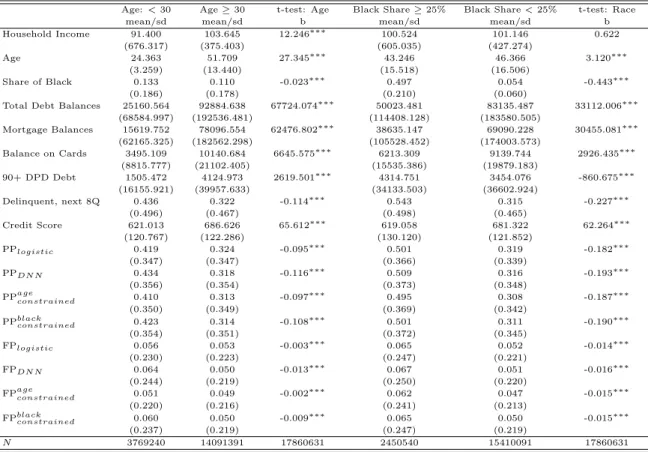
We report descriptive statistics for this exercise in Table 6. We can see that young borrowers default on their loans at slightly higher rates, have lower debt and 90+ dpd debt balances, lower household income, and ranked lower in both the credit scores and our model’s risk distribution. The cross-group differences are similar in direction but even larger in magnitude for the first income quantile vs. the rest comparison.
To complement Table 6, Panel (a) of Figure 6 plots the average difference across age and across default status, while Panel (b) displays these differences over time. We can see that the introduction of our hybrid model would mostly benefit young borrowers. For instance, the raw difference of 2 units for the youngest age group translates into improved credit ranking by 2 percentiles, which would improve their access to credit markets. Additionally, individuals who do not default would on average benefit across all age groups.
We report the regression results in Table 7. Columns (1) shows that precisely the most vulnerable subgroup, young individuals whose income is in the bottom quintile of the income distribution benefit the most from our credit risk model. In particular, our model would rank these individuals by 3.3 percentile higher on average in the credit risk distribution. We then control for default status, and while Column (2) shows that every borrower who do not end up defaulting would gain from our credit risk assessment, young and low income no-defaulters would be the largest beneficiaries, being ranked 5.2 percentile higher by our hybrid model. Columns (3-4) show that the benefits are similar in areas hard hit by unemployment shocks. This result holds during the Great Recession (i.e, 2007-2009), and the interpretation of this is that, relative to other groups, our model provides more favorable credit risk assessment for
credit scores do not provide an exact probability of default, we are unable to conclude whether our model would provide a larger number of borrowers access to credit (i.e., the extensive margin) across age and income groups in the borrower population. However, contrasting the relative ranking reiterates the notion that credit scores are indiscriminately low for young and low income borrowers.
1.5.4 Mortgage Default
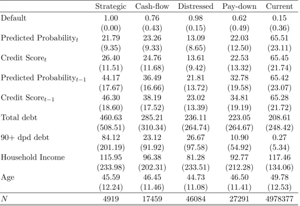
We next compare our model with credit scores in predicting various categories of mort-gage default. We restrict our sample to borrowers with mortmort-gage debt and use the same percentile ranking as described in Section 1.5.3. We further restrict our sample to individu-als who show new mortgage delinquency (i.e., current on all mortgage debt in the previous quarter), and who have debt outstanding aside from mortgage debt. We classify mortgage default into four categories: strategic, distressed, cash-flow, pay-down. We also include in-dividuals who do not show any sign of mortgage delinquency throughout this period as our benchmark group.18 The main caveat of this approach is our inability to distinguish between
default due to income constraints and negative equity. For true strategic default, negative equity is a necessary condition, which we cannot control for. The magnitude of this bias was investigated by [19]. They show that between 2008 and 2011 the fraction of strategic defaulters accounted for 21% of all defaulters, of which 15.5% were truly strategic defaulters. We report descriptive statistics for this exercise in Table 9. We can see that strategic defaulters have both the highest debt and 90 days late debt balances. One striking difference between our ranking and credit scores is the treatment of strategic defaulters. While credit scores rank them as the second least risky group, we rank them as the fourth.
We now estimate regressions as in Equation (1.4), with our interaction variables be-ing default status and mortgage default type. Table 10 reports the results. In Column (1-3) our dependent variable is the quarter in which the borrower shows no delinquency 18These categories largely correspond to the work of Experian-Oliver Wyman (2009). Nonethe-less, we are more stringent on classifying strategic default by requiring no delinquency on any other debt in the two consecutive quarters after showing mortgage delinquency, instead of requiring it only two quarters ahead. See https://www.experian.com/assets/decision-analytics/reports/ strategic-default-report-1-2009.pdf.
on mortgage debt. Column (1-2) show that our model would rank strategic defaulters by approximately 2.5 percentiles lower on average in the quarter they yet to show a sign of mortgage delinquency. Given that our benchmark group is the “current” group, the con-stant in our regression illustrates that borrowers who stay current and do not default in the subsequent two years would be ranked 1 percentile higher on average. We next look at ranking differences in the quarter they become delinquent on their mortgage debt. Column (4) and (5) show that strategic defaulters would be ranked by approximately 5 percentile lower19, and that all other groups who do not default would be ranked higher according to
our model. Column (3) and (6) repeats the ranking exercise with lag and contemporaneous ranking for the Great Recession sample. The overall results are largely similar, however, we see an even larger gain for borrowers who do not default in the subsequent two years being ranked by approximately 2 percentile higher in the credit risk distribution on average. These results reaffirm the findings of [5], that is, credit scores did not accurately reflect the probability of default for a large group of mortgage owners during the 2007-2009 housing crisis. This misclasification is particularly severe for strategic defaulters.
1.6 Applications
In this section, we use our model in two applications. We first show that our model is able to accurately predict variations in aggregate default risk, and second, we illustrate the value added for lenders and borrowers from our hybrid model.
1.6.1 Predicting Systemic Risk
We first analyze the aggregate forecasting power of our hybrid model. We aggregate the deep-learning forecasts for individual accounts to generate macroeconomic forecasts of credit risk by taking the average of the predicted probabilities over a given forecast period. Since our sample of consumers in nationally representative in each quarter, this will provide
an unbiased estimate of the aggregate default risk predicted by our model. We calculate the aggregate default probability for 2006Q1-2013Q4, and show that our model is able to predict the spike in delinquencies during the 2007-2009 financial crisis and also the reduction in delinquencies since then. This estimate of aggregate default risk could be used as a proxy of systemic risk in the household sector. The results are displayed in Figure 7.
Panel (a) plots the aggregate predicted default rate from our hybrid model and compares it to the aggregate realized default rate. While our predicted aggregate default rate is approximately 2 percentage points lower than the realized in 2006 and 2007, it rises at a similar speed as the realized default rate. It peaks in 2010Q2, approximately 2 quarters after the peak in the realized rate and then declines in the ensuing period, again reflecting the behavior of the realized rate, though it overestimates it by about 1 percentage point. Panel (b) shows a scatter plot of the predicted aggregate default rate against the realized for the different quarters in our sample period. The correlation between the predicted and realized aggregate default rate is 62%.
1.6.2 Value Added
We assess the economic salience of our hybrid DNN-GBT model by analyzing its value added for lenders and borrowers. For lenders, we examine the role our model can play in minimizing the losses from default. For borrowers, we calculate the interest savings for borrowers who are misclassified as having an excessively high probability of default based on the credit score compared to our model.
1.6.2.1 Lenders We follow the framework proposed by [55], which compares the value of having a prediction of default risk to having none, and we make the same simplifying assump-tions with respect to the revenues and costs of the consumer lending business. Specifically, in absence of any forecasts, it is assumed a lender will take no action regarding credit risk, implying that customers who default will generate losses for the lender, and customers who are current on their payments will generate positive revenues from financing fees on their running balances. To simplify, we assume that all defaulting and non-defaulting customers
have the same running balance, Br, but defaulting customers increase their balance to Bd prior to default. We refer to the ratio between Bd and Br as “run-up.” It is assumed that with a model to predict default risk, a lender can avoid losses of defaulting customers by cutting their credit line and avoiding run-up. Then, the value added as proposed by [55] can be written as follows: V A(r, N, T N, F N, F P) = T N −F N 1−(1 +r)−NBd Br −1 −1 T N +F P (1.5)
wherer refers to the interest rate,N the loan’s amortization period, andT N, F N, F P refer to true negatives, false negatives and false positives respectively. Panel (a) of Figure 8 plots the Value Added (VA) as a function of interest rate and the ratio of run-up balance for our out-of-sample forecasts of 90+ days delinquencies over the subsequent 8 quarters for 2012Q4. These estimates imply cost savings of over 60% of total losses when compared to having no forecast model for a run-up of 1.2 at a 10% interest rate for an amortization period for 3 years.
We next compare the value added of our hybrid model with default predictions generated by a logistic regression. This exercise illustrates the gains from adopting a better technology for credit allocation. Panel (b) of Figure 8 shows more modest, but substantial cost savings in the range of 1-6% and approximately 2.5% for a 1.2 run-up at a 10% interest rate with a 3 year amortization period. Panel (c) calculates the cost savings associated to using our hybrid model in comparison to random forest. In this case the cost savings range from 0.1-0.7%. This exercise then confirms the advantages of using deep learning over other technologies in predicting default.
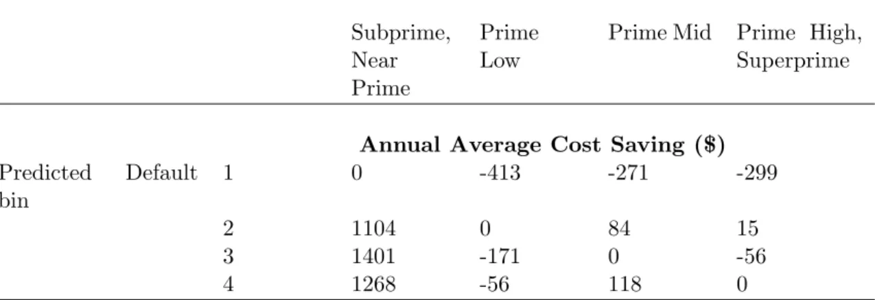
1.6.2.2 Borrowers We now examine the potential cost savings for consumers who would be offered credit according to the predicted default probability implied by our model instead of a conventional credit score. Following our approach in Section 1.5, we create credit score categories based on common industry standards and corresponding predicted probability bins with the same number of observations for each quarter, and we place customers in