PhD-FSTC-2015-39
Faculté des Sciences, de la Technologie et de la Communication
DISSERTATION
Defense held on15/09/2015in Luxembourg
to obtain the degree of
DOCTEUR DE L’UNIVERSITÉ DU LUXEMBOURG
EN INFORMATIQUE
by
Alejandro CORREA BAHNSEN
Born on March18,1985in Bogota, Colombia
E X A M P L E - D E P E N D E N T C O S T - S E N S I T I V E
C L A S S I F I C AT I O N
a p p l i c at i o n s i n f i na n c i a l r i s k m o d e l i n g
a n d m a r k e t i n g a na ly t i c s
D
issertation defense committee
Dr BjörnOttersten, dissertation supervisor
Professor, Université du Luxembourg
Dr DjamilaAouada, dissertation co-supervisor
Research Scientist, Université du Luxembourg
Dr YvesLeTraon, Chairman Professor, Université du Luxembourg
Dr BartDeMoor, Vice Chairman Professor, Katholieke Universiteit Leuven
Dr GianlucaBontempi
A B S T R A C T
Several real-world binary classification problems are example-dependent cost-sensitive in nature, where the costs due to misclassifica-tion vary between examples and not only within classes. However, stan-dard binary classification methods do not take these costs into account, and assume a constant cost of misclassification errors. This approach is not realistic in many real-world applications. For example in credit card fraud detection, failing to detect a fraudulent transaction may have an economical impact from a few to thousands of Euros, depending on the particular transaction and card holder. In churn modeling, a model is used for predicting which customers are more likely to abandon a service provider. In this context, failing to identify a profitable or un-profitable churner has a significant different economic result. Similarly, in direct marketing, wrongly predicting that a customer will not accept an offer when in fact he will, may have different financial impact, as not all customers generate the same profit. Lastly, in credit scoring, accept-ing loans from bad customers does not have the same economical loss, since customers have different credit lines, therefore, different profit.
Accordingly, the goal of this thesis is to provide an in-depth analysis of example-dependent cost-sensitive classification. We analyze four real-world classification problems, namely, credit card fraud detection, credit scoring, churn modeling and direct marketing. For each problem, we propose an example-dependent cost-sensitive evaluation measure.
We propose four example-dependent cost-sensitive methods; the first method is a cost-sensitive Bayes minimum risk classifier which consists in quantifying tradeoffs between various decisions using probabilities and the costs that accompany such decisions. Second, we propose a cost-sensitive logistic regression technique. This algorithm is based on a new logistic regression cost function; one that takes into account the real costs due to misclassification and correct classification. Subsequently, we propose a cost-sensitive decision trees algorithm which is based on incorporating the different example-dependent costs into a new cost-based impurity measure and a new cost-cost-based pruning criteria. Lastly, we define an example-dependent cost-sensitive framework for ensem-bles of decision-trees. It is based on training example-dependent cost-sensitive decision trees using four different random inducer methods and then blending them using three different combination approaches. Moreover, we present the library CostCla developed as part of the
sis. This library is an open-source implementation of all the algorithms covered in this manuscript.
Finally, the experimental results show the importance of using the real example-dependent financial costs associated with real-world ap-plications. We found that there are significant differences in the results when evaluating a model using a traditional cost-insensitive measure such as accuracy or F1Score, than when using the financial savings.
Moreover, the results show that the proposed algorithms have better results for all databases, in the sense of higher savings.
To my wife Alejandra
A C K N O W L E D G M E N T S
First and foremost, I would like to sincerely thank my advisor Prof. Dr. Björn Ottersten for the continuous support during my Ph.D study and research, for his motivation, enthusiasm, and for the freedom I was granted throughout these years.
My sincere thanks also goes to my co-advisor Dr. Djamila Aouada for her support, guidance, and encouragement not only from the research point of view, but for life in general.
Deepest gratitude are also due to all members of the jury for their interest in this work and for taking the time to evaluate this dissertation. Special thanks go to the fraud management team at CETREL a SIX Company. In particular to Guy Weber and Philippe Davin, for all the time they invest in helping me understand all the particularities of the credit card fraud detection problem. Moreover, for their insights during the different steps of my research.
I would also like to convey thanks for supporting this Ph.D project to the AFR Grant Scheme (Aides la Formation-Recherche), managed by the National Research Fund of Luxembourg (FNR).
I cannot finish without saying how grateful I am with my wife Ale-jandra and son Pablo. They have always supported and encouraged me to do my best in all matters of life.
C O N T E N T S n o tat i o n s xiii a c r o n y m s xv l i s t o f ta b l e s xvi l i s t o f f i g u r e s xix 1 i n t r o d u c t i o n 1
1.1 Motivation and scope . . . 1
1.2 Contributions . . . 3 1.3 Outline . . . 4 1.4 Publications . . . 5 I e x a m p l e-d e p e n d e n t c o s t-s e n s i t i v e c l a s s i f i c at i o n 7 2 b a s i c s o n c l a s s i f i c at i o n 9 2.1 Introduction . . . 9
2.2 Traditional evaluation measures . . . 11
2.2.1 Brier score . . . 14
3 c o s t-s e n s i t i v e c l a s s i f i c at i o n 15 3.1 Introduction . . . 15
3.2 Class-dependent cost-sensitive classification . . . 16
3.3 Example-dependent cost-sensitive classification . . . 17
3.3.1 Example-dependent evaluation measures . . . 18
3.3.2 Binary classification cost characteristic . . . 21
3.3.3 State-of-the-art methods . . . 22
II r e a l-w o r l d e x a m p l e-d e p e n d e n t a p p l i c at i o n s 23 4 f i na n c i a l r i s k m o d e l i n g 25 4.1 Credit card fraud detection . . . 25
4.1.1 Credit card fraud detection evaluation . . . 27
4.1.2 Feature engineering for fraud detection . . . 28
4.1.3 Database . . . 35
4.2 Credit scoring . . . 35
4.2.1 Financial evaluation of a credit scorecard . . . 36
4.2.2 Databases . . . 39
4.3 Summary of the datasets . . . 40
5 m a r k e t i n g a na ly t i c s 43 5.1 Churn modeling . . . 43
5.1.1 Flow analysis of a churn campaign . . . 44
5.1.2 Propose evaluation measure of a churn campaign . 46
x c o n t e n t s
5.1.3 Churn modeling database . . . 49
5.2 Direct marketing . . . 50
5.3 Summary of the datasets . . . 51
III p r o p o s e d e x a m p l e-d e p e n d e n t c o s t-s e n s i t i v e m e t h o d s 53 6 b ay e s m i n i m u m r i s k 55 6.1 Bayes minimum risk model . . . 55
6.2 Calibration of probabilities . . . 56
6.2.1 Calibration due to a change in base rates . . . 56
6.2.2 Calibration using the ROC convex hull . . . 56
6.3 Experiments . . . 58
7 c o s t-s e n s i t i v e l o g i s t i c r e g r e s s i o n 63 7.1 Logistic regression . . . 63
7.2 Cost-sensitive logistic regression . . . 64
7.2.1 Implicit costs of the logistic regression . . . 64
7.2.2 Cost-sensitive logistic regression cost function . . . 65
7.3 Experiments . . . 66
8 c o s t-s e n s i t i v e d e c i s i o n t r e e s 69 8.1 Introduction . . . 69
8.2 Decision trees . . . 70
8.2.1 Construction of classification trees . . . 70
8.2.2 Decision tree algorithms . . . 75
8.3 Example-Dependent Cost-sensitive Decision Trees . . . 75
8.3.1 Cost-sensitive impurity measures . . . 75
8.3.2 Cost-sensitive pruning . . . 76
8.4 Experiments . . . 77
9 e n s e m b l e s o f c o s t-s e n s i t i v e d e c i s i o n t r e e s 83 9.1 Introduction . . . 83
9.2 Ensemble methods . . . 84
9.2.1 Theoretical performance of an ensemble . . . 85
9.3 Ensembles of cost-sensitive decision trees . . . 86
9.3.1 Random inducers . . . 86
9.3.2 Combination methods . . . 87
9.3.3 Algorithms . . . 89
9.4 Theoretical analysis of the ECSDT . . . 90
9.5 Experiments . . . 93
10 c o n c l u s i o n s 103 10.1 Future research directions . . . 104
a costcla: a c o s t-s e n s i t i v e c l a s s i f i c at i o n l i b r a r y i n python 107 a.1 Library overview . . . 107
c o n t e n t s xi
a.2 Usage . . . 108
a.3 Installation . . . 110
N O TAT I O N S
S Set of examples
Strain Training set
Stest Testing set
S0 Set of negative examples
S1 Set of positive examples
y Vector of class labels
xi Feature vector of examplei k Number of features
N Number of examples inS
N0 Number of negative examples in S0 N1 Number of positive examples inS1 yi Class label of examplei
π0 Percentage of negative examples inS π1 Percentage of positive examples in S f(S) A classification algorithm
fa(S) Function that classifies every example asa
c Predicted class labels
ci Predicted class for examplei ˆ
pi Predicted probability of positive for examplei t Probability threshold
T P Number of true positives examples T N Number of true negatives examples FP Number of false positives examples FN Number of false negatives examples CFP Cost of a false positive
CFN Cost of a false negative
CT Pi Cost of a true positive for examplei CT Ni Cost of a true negative for example i CFPi Cost of a false positive for examplei CFNi Cost of a false negative for example i x∗i Augmented feature vector of examplei
xiv c o n t e n t s
1c(z) Indicator function that takes the value of one if z ∈ c and
zero ifz /∈c
|§| Cardinality of a set§
bi Classification problem cost characteristic µb Mean of the classification cost characteristic
σb Standard deviation of the classification cost characteristic Ca Administrative cost of contacting a customer
Amti Amount of transactioni
tp Number of hours to aggregate transactions xidi Customer who made transactioni
xtimei Time of transactioni
intr Annual interest rate charged to a customer Lgd Credit scoring loss given default
ri Expected profit of customeri CLi Credit line of customeri li Term of the loan of customeri
intcf Cost of funds of a financial institution debti Outstanding debt of customer i
γ Probability of accepting an offer CLV Average customer lifetime value CLVi Customer lifetime value of examplei Coi Cost of making an offer to customeri Inti Expected profit generated by customeri θ Parameters of the logistic regression hθ Logistic regression hypothesis J(θ) Logistic regression cost function
Jc(θ) Cost-sensitive logistic regression cost function lj Splitting rule of a decision tree
I Impurity measure of a decision tree T ree A decision tree
A C R O N Y M S CS Cost-sensitive classification CI Cost-insensitive classification CPS Cost-proportionate sampling CST Cost-sensitive training LR Logistic regression DT Decision tree RF Random forest BMR Bayes minimum risk
CSLR Cost-sensitive logistic regression CSDT Cost-sensitive decision tree
ECSDT Ensemble of cost-sensitive decision tree CSB Cost-sensitive bagging
CSP Cost-sensitive pasting
CSRF Cost-sensitive random forest CSRP Cost-sensitive random patches
t Training
u Under-sampling
r Cost-proportionate rejection-sampling o Cost-proportionate over-sampling mv Majority voting
wv Cost-sensitive weighted voting s Cost-sensitive stacking
L I S T O F TA B L E S
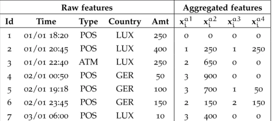
Table2.1 Classification confusion matrix . . . 12 Table3.1 Classification cost matrix . . . 18 Table3.2 Simplified classification cost matrix [Elkan, 2001] . 18 Table4.1 Credit card fraud cost matrix . . . 28 Table4.2 Summary of typical raw credit card fraud
detec-tion features . . . 29 Table4.3 Example calculation of aggregated features. For
all aggregated features tp =24. . . 31 Table4.4 Example calculation of periodic features. . . 34 Table4.5 Credit scoring example-dependent cost matrix . . 37 Table4.6 Credit scoring model parameters . . . 40 Table4.7 Summary of the financial datasets, whereNis the
number of examples and π1 is the percentage of
positive examples. . . 41 Table5.1 Proposed churn modeling example-dependent
cost matrix . . . 47 Table5.2 Direct marketing example-dependent cost matrix . 50 Table5.3 Summary of the marketing datasets, where N is
the number of examples andπ1 is the percentage of positive examples. . . 51 Table6.1 Results of the algorithms measured by savings . . 59 Table6.2 Results of the algorithms measured by Brier score 61 Table7.1 Logistic regression cost matrix . . . 65 Table7.2 Results of the algorithms measured by savings . . 68 Table7.3 Results of the algorithms measured by F1Score . . 68 Table8.1 Results on the three datasets of the
cost-sensitive and standard decision tree, with-out pruning (notp), with error based prun-ing (errp), and with cost-sensitive pruning technique (costp). Estimated using the dif-ferent training sets: training, under-sampling, proportionate rejection-sampling and cost-proportionate over-sampling . . . 78
xviii List of Tables
Table8.2 Training time and tree size of the different
cost-sensitive and standard decision tree, estimated using the different training sets: training, under-sampling, cost-proportionate rejection-sampling and cost-proportionate over-sampling, for the three databases. . . 80 Table9.1 Results of the CI and BMR algorithms measured
by savings . . . 94 Table9.2 Results of the CST and ECSDT algorithms
mea-sured by savings . . . 95 Table9.3 Savings Friedman ranking and average
percent-age of best result . . . 96 Table9.4 Savings ranks of best algorithm of each family by
database . . . 97 Table9.5 Results of the CI and BMR algorithms measured
by F1Score . . . 101
Table9.6 Results of the CST and ECSDT algorithms
mea-sured byF1Score. . . 102 Table A.1 Results of the different algorithms using the
L I S T O F F I G U R E S
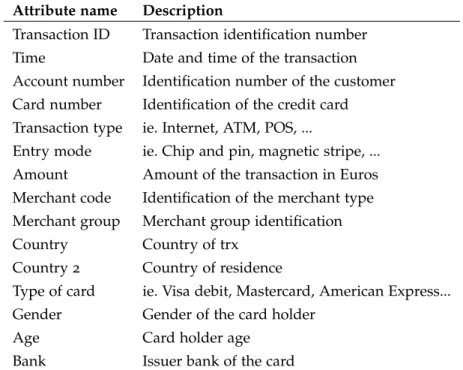
Figure1.1 Different example-dependent cost-sensitive
algo-rithms grouped according to the stage in a classi-fication system where they are used. . . 2 Figure2.1 Classification process . . . 10 Figure2.2 Example of a classification algorithm. Using a set
of examples from two classes, a classification al-gorithm is learned in order to separate between the positives and the negatives. . . 11 Figure2.3 Example of a classification algorithm. Using a set
of examples from two classes, a classification al-gorithm is learned in order to separate between the positives and the negatives. . . 13 Figure3.1 Class-dependent cost-sensitive classification
al-gorithm. Since the cost of misclassifying positives and negatives is different, the algorithm focus on maximizing the correct classification of the posi-tives. . . 17 Figure3.2 Example with example-dependent costs.
Exam-ples with the highest cost in darker colors, and the ones with the lowest cost are in lighter colors. 20 Figure3.3 Example-dependent cost-sensitive classification
algorithm. The algorithm focus first on correctly classify the dark examples, as the cost of misclas-sification in this cases is several times more ex-pensive than the other cases. . . 20 Figure4.1 Analysis of the time of a transaction using a 24
hour clock. The arithmetic mean of the transac-tions time (dashed line) do not accurately repre-sents the actual times distribution. . . 32 Figure4.2 Fitted von Mises distribution including the
peri-odic mean (dashed line) and the probability dis-tribution (purple area). . . 33 Figure4.3 Expected time of a transaction (green area).
Us-ing the confidence interval, a transaction can be flag normal or suspicious, depending whether or not the time of the transaction is within the con-fidence interval. . . 34
xx List of Figures
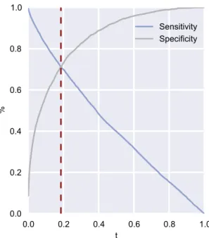
Figure4.4 Credit scoring sensitivity versus specificity
thresholding procedure. . . 36 Figure5.1 Flow analysis of a churn campaign [Verbraken,
2012] . . . 45 Figure5.2 Financial impact of the different decisions, i.e.,
False positives, false negatives, true positives and true negatives . . . 46 Figure5.3 Acceptance rate (γ) of the best offer for each
cus-tomer profile. As expected, the higher the churn rate the lower the acceptance rate, as it is more difficult to make a good offer to a customer which is more likely to defect. . . 50 Figure6.1 Estimation of calibrated probabilities using the
ROC convex hull. . . 57 Figure6.2 Comparison of the average savings of the
algo-rithms versus the highest savings by family of classifiers. When the probabilities are calibrated there is a significant increase in savings. . . 60 Figure6.3 Comparison of the average Brier score of the
al-gorithms versus the lowest Brier score by family of classifiers. Overall, the models that are cali-brated are indeed the ones with the best Brier score. 62 Figure7.1 Sigmoid function . . . 64 Figure7.2 Comparison of the average savings andF1Score
of the algorithms versus the the best model. The models that perform the best measured by F1Scoreare not the best in terms of savings. . . 67 Figure8.1 Impurity measures for a binary classification, as
a function of the proportion of positive examples in the set (Cross-entropy is scaled) [Hastie et al., 2009]. . . 71 Figure8.2 Results of the DT and the CSDT. For both
algo-rithms, the results are calculated with and with-out both types of pruning criteria. . . 79 Figure8.3 Average savings on the three datasets of the
different cost-sensitive and standard decision tree, estimated using the different training sets: training, under-sampling, cost-proportionate rejection-sampling and cost-proportionate over-sampling. . . 79 Figure8.4 Average tree size (a) and training time (b), of
the different cost-sensitive and standard decision tree, estimated using the different training sets. . . 81
List of Figures xxi
Figure9.1 Main reasons regarding why ensemble
meth-ods perform better than single models: statistical, computational and representational [Dietterich, 2000]. . . 85 Figure9.2 Visual representation of the random inducers
al-gorithms. . . 87 Figure9.3 Comparison of the savings of the algorithms
versus the highest savings in each database.The CSRP −wt is very close to the best result in all the databases. Additionally, even though the LR−BMR is the best algorithm in two databases, the performance in the other three is very poor. . . 97 Figure9.4 Comparison of the results by family of
clas-sifiers. The ECSDT family has the best perfor-mance measured either by Friedman ranking or average percentage of best model. . . 98 Figure9.5 Comparison of the Friedman ranking within
the ECSDT family. Overall, the random inducer method that provides the best results is theCSRP. Moreover, the best combination method com-pared by Friedman ranking is the cost-sensitive weighted voting. . . 99 Figure9.6 Comparison of the Friedman ranking of the
sav-ings and F1Score sorted by F1Score ranking.The best two algorithms according to their Friedman rank of F1Score are indeed the best ones
mea-sured by the Friedman rank of the savings. How-ever, this relation does not consistently hold for the other algorithms as the correlation between the rankings is just 65.10%. . . 100
1
I N T R O D U C T I O N
1.1 m o t i vat i o n a n d s c o p e
Classification, in the context of machine learning, deals with the prob-lem of predicting the class of a set of examples given their features. Traditionally, classification methods aim at minimizing the misclassifi-cation of examples in which an example is misclassified if the predicted class is different from the true class. Such a traditional framework as-sumes that all misclassification errors carry the same cost. This is not the case in many real-world applications. Methods that use different misclassification costs are known as cost-sensitive classifiers. Typical cost-sensitive approaches assume a constant cost for each type of er-ror, in the sense that, the cost depends on the class and is the same among examples [Elkan,2001; Kim et al.,2012].
This class-dependent approach is not realistic in many real-world ap-plications. For example in credit card fraud detection, failing to detect a fraudulent transaction may have an economical impact from a few to thousands of Euros, depending on the particular transaction and card holder [Ngai et al., 2011]. In churn modeling, a model is used for pre-dicting which customers are more likely to abandon a service provider. In this context, failing to identify a profitable or unprofitable churner has a significant different economic result [Verbraken et al., 2013]. Sim-ilarly, in direct marketing, wrongly predicting that a customer will not accept an offer when in fact he will, may have different financial impact, as not all customers generate the same profit [Zadrozny et al., 2003]. Lastly, in credit scoring, accepting loans from bad customers does not have the same economical loss, since customers have different credit lines, therefore, different profits [Verbraken et al., 2014].
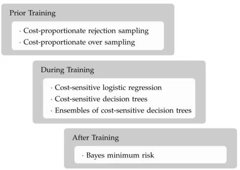
Methods that use different misclassification costs are known as cost-sensitive classifiers. In particular, we are interested in methods that are example-dependent cost-sensitive, in the sense that the costs vary among examples and not only among classes [Elkan, 2001]. However, the literature on example-dependent cost-sensitive methods is limited, mostly because there is a lack of publicly available datasets that fit the problem [Aodha and Brostow,2013]. Example-dependent cost-sensitive classification methods can be grouped according to the step where the costs are introduced into the system. Either the costs are introduced prior to the training of the algorithm, after the training or during
2 i n t r o d u c t i o n
Prior Training
During Training
After Training
·Cost-proportionate rejection sampling
·Cost-proportionate over sampling
·Cost-sensitive logistic regression
·Cost-sensitive decision trees
·Ensembles of cost-sensitive decision trees
· Bayes minimum risk
Figure1.1: Different example-dependent cost-sensitive algorithms grouped
ac-cording to the stage in a classification system where they are used.
ing [Wang, 2013]. In Figure 1.1, the different algorithms are grouped according to the stage in a classification system where they are used.
The first set of methods that were proposed to deal with cost-sensitivity consist in re-weighting the training examples based on their costs, either by cost-proportionate rejection-sampling [Zadrozny et al., 2003], or cost-proportionate over-sampling [Elkan, 2001]. The rejection-sampling approach consists in randomly selecting examples from a training set, and accepting each example with probability equal to the normalized misclassification cost of the example. On the other hand, the over-sampling method consists in creating a new set, by making n copies of each example, wheren is related to the normalized misclassi-fication cost of the example. These methods however, fail to introduce the example-dependent cost to the training of the different algorithms, and only rely on modifying the prior distribution of the training data.
The focus of this thesis is to investigate and define different example-dependent cost-sensitive classification algorithms, that not only focus on modifying the distribution of the training data but also introduce the different real financial costs during the training of the algorithms. We summarize the contributions of this thesis in the following section.
1.2 c o n t r i b u t i o n s 3
1.2 c o n t r i b u t i o n s
This dissertation summarizes several contributions to the field of example-dependent cost-sensitive machine learning.
(a) Cost-sensitive financial evaluation measure
Binary classification algorithms are normally evaluated using cost-insensitive evaluation measures, such as misclassification rate or F1Score. However, these measures may not be the most
appropri-ate evaluation criteria when evaluating real-world cost-sensitive problems, because they tacitly assume that misclassification er-rors carry the same cost. In this thesis, we propose a new sav-ings example-dependent cost-sensitive evaluation measure. The savings take into account the actual financial impact of the differ-ent misclassification errors. This work was published in [Correa Bahnsen et al., 2013].
(b) Cost-sensitive credit card fraud detection
Preventing credit card fraud is a classical example of a cost-sensitive problems, as the cost of a false negative is significantly different than the cost of a false positive. We discuss the partic-ularities of credit card fraud detection and propose a financial evaluation measure that takes into account the economical costs associated with credit card fraud. Moreover, we propose to create a new set of features based on analyzing the periodic behavior of the time of a transaction using a modelling with a von Mises dis-tribution. This work was published in [Correa Bahnsen et al.,2013, 2014b] and is under review inCorrea Bahnsen et al.[2015d,e].
(c) Example-dependent cost-sensitive real-world problems
We analyze and propose financial evaluation measures for other real-world applications, namely, credit card fraud detection , churn modeling and direct marketing. The different analyses were presented in [Correa Bahnsen et al., 2014b,a, 2015b].
(d) Cost-sensitive Bayes minimum risk
In this thesis we propose a direct cost approach to make the clas-sification decision based on the expected costs. This method is an extension of Bayes minimum risk, and consists in quantifying tradeoffs between various decisions using probabilities and the costs that accompany such decisions. This model was published in [Correa Bahnsen et al., 2013,2014b].
(e) Cost-sensitive logistic regression and decision trees
4 i n t r o d u c t i o n
the training of an algorithm, leaving opportunities to investigate the potential impact of algorithms that take into account the real financial example-dependent costs during the training of an al-gorithm. We propose a new cost-sensitive logistic regression. The method consists in introducing example-dependent costs into a lo-gistic regression, by changing the objective function of the model to one that is cost-sensitive. We then apply a similar approach by introducing the costs in a cost-sensitive decision tree. The method is based on a new splitting criteria which is cost-sensitive, used during the tree construction. These methods were published in [Correa Bahnsen et al., 2014a,2015a].
(f) Ensembles of cost-sensitive decision trees
Based on the cost-sensitive decision tree algorithm, we expand the cost-sensitive decision trees by creating a framework for an ensem-ble of cost-sensitive decision trees. This new method, step on the advantages of ensemble learning in order to create a more robust model. This work was submitted for review [Correa Bahnsen et al., 2015c].
(g) CostCla: A cost-sensitive classification library
The algorithms developed as part of this thesis are publicly avail-able as part of the open-sourceCostSensitiveClassification1
library.
1.3 o u t l i n e
Part I of this manuscript is focused on giving the general concepts of classification and cost-sensitive classification. In particular, in Chap-ter 2, we give a background on classification. Then, in Chapter 3, we present the cost-sensitive problem and define the difference between cost-insensitive, class-dependent cost-sensitive and example-dependent cost-sensitive classification problems. Lastly, we give an introduction of the different evaluation measures used throughout this thesis.
Part II is dedicated to explaining the particularities of the four real-world classification problems that are the focus of this thesis, in par-ticular, credit card fraud detection, credit scoring, churn modeling and direct marketing. In general, we show why each of the applications is example-dependent cost-sensitive, and we elaborate a framework for the analysis of each problem. This part is organized in two chapters. First, in Chapter 4, we discuss the applications within financial risk management. Second, in Chapter5, we analyze marketing analytics ap-plications.
1.4 p u b l i c at i o n s 5
Part III is focused on introducing our proposed example-dependent cost-sensitive methods. First, in Chapter 6, we present the Bayes mini-mum risk method. Then, we introduce the cost-sensitive logistic regres-sion algorithm in Chapter 7. Afterwards, in Chapter 8, we show and discuss the cost-sensitive decision trees algorithm. Lastly, in Chapter 9, we present our framework for ensembles of cost-sensitive decision trees. Chapter 10 concludes the thesis, and elaborates on possible lines for future research. Lastly, in the Appendix A, we present the library CostCla developed as part of the thesis. This library is an open-source implementation of all the algorithms covered in this manuscript.
1.4 p u b l i c at i o n s
Publications from this work are:
(a) [Correa Bahnsen et al.,2013]Cost Sensitive Credit Card Fraud Detec-tion Using Bayes Minimum Risk, Alejandro Correa Bahnsen, Alek-sandar Stojanovic, Djamila Aouada and Björn Ottersten. In Pro-ceedings of IEEE International Conference on Machine Learning and Applications,2013.
(b) [Correa Bahnsen et al.,2014b]Improving Credit Card Fraud Detection with Calibrated Probabilities, Alejandro Correa Bahnsen, Aleksandar Stojanovic, Djamila Aouada and Björn Ottersten. In Proceedings of SIAM International Conference on Data Mining,2014.
(c) [Correa Bahnsen et al., 2014a] Example-Dependent Cost-Sensitive Logistic Regression for Credit Scoring, Alejandro Correa Bahnsen, Djamila Aouada and Björn Ottersten. In Proceedings of IEEE Inter-national Conference on Machine Learning and Applications,2014.
(d) [Correa Bahnsen et al.,2015a]Example-Dependent Cost-Sensitive De-cision Trees, Alejandro Correa Bahnsen, Djamila Aouada and Björn Ottersten. In Expert Systems with Applications, 42(19):6609-6619,
2015.
(e) [Correa Bahnsen et al., 2015b] A novel cost-sensitive framework for customer churn predictive modeling, Alejandro Correa Bahnsen, Djamila Aouada and Björn Ottersten. In Decision Analytics,2(1):5,
2015.
(f) [Correa Bahnsen et al., 2015c] Ensembles of Example-Dependent Cost-Sensitive Decision Trees, Alejandro Correa Bahnsen, Djamila Aouada and Björn Ottersten. Submitted to IEEE Transactions on Knowledge and Data Engineering,2015.
6 i n t r o d u c t i o n
(g) [Correa Bahnsen et al., 2015d] Feature Engineering in Credit Card Fraud Detection, Alejandro Correa Bahnsen, Djamila Aouada and Björn Ottersten. Submitted to Expert Systems with Applications,
2015.
(h) [Correa Bahnsen et al., 2015e] Detecting Credit Card Fraud using Periodic Features, Alejandro Correa Bahnsen, Djamila Aouada and Björn Ottersten. Submitted to the IEEE International Conference on Machine Learning and Applications,2015.
Part I
E X A M P L E - D E P E N D E N T C O S T - S E N S I T I V E
C L A S S I F I C AT I O N
2
B A S I C S O N C L A S S I F I C AT I O N
Outline
In this chapter, we introduce classification models from a machine learn-ing perspective. First, in Section 2.1, we give a self contained intro-duction to classification, including the most-common algorithms, and the main applications of classification models. Then, in Section 2.2, we present the different evaluation measures that are normally used for analyzing the performance of classification methods.
2.1 i n t r o d u c t i o n
In machine learning, classification refers to the attempt of identifying to which of a set of classes a new example belongs, based on learning from examples whose class membership is known. A classification task begins with a training set in which the class of a set of examples is known. For example, a classification model that predicts credit card fraud is developed by analyzing many observed credit transactions over a period of time. The class in this case is a variable which indicates for each example whether or not the transaction was or not a fraud. Also, the features, are the transaction attributes like place, amount and time of the transaction.
Then, during the training process, a classification algorithm finds the patterns and relationships between the values of the features and the values of the target class. Different algorithms use different methods and techniques to estimate these relationships. Afterwards, these rela-tionships are summarized in a model that is able to make predictions on new sets of data.
In general, there are two types of classification models: binary and multi-class. In binary classification problems, the objective is to classify examples between two classes, usually referred to as the negative and positive classes. On the other hand, multi-class problems are not bound to two classes but instead aim to classify examples among a number of classes. In this work we focus on binary classification problems.
Binary classification algorithms are widely used across a variety of domains. For example in the medical field, models have been used for making predictions about tumors, probability of a disease, probability of selecting the right drug for a particular patient, and estimating the
10 b a s i c s o n c l a s s i f i c at i o n
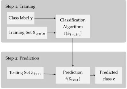
Step1: Training
Step2: Prediction
Class labely
Training SetStrain
Classification Algorithm
f(Strain)
Testing SetStest Prediction
f(Stest)
Predicted
classc
Figure2.1: Classification process
probability of relapsing, among others [Herland et al., 2014]. In the fi-nancial sector, classification models have been successfully applied for fraud detection, credit scoring, portfolio management and algorithmic trading. Also, in marketing, several models are being currently used for churn modeling, customer targeting, behavior prediction and direct marketing [Baesens, 2014]. Additionally, classification algorithms are used in many other emerging applications such as terrorism prevention, malware detection, computer security, energy consumption prediction, spam classification, and others [Kriegel et al., 2007].
Formally, a binary classification algorithm deals with the problem of predicting the class yi of a set S of examples or instances i, given
theirkfeaturesxi ∈Rk. The objective is to construct a functionf(S)that
makes a prediction ci of the class of each example i from S using its feature vector xi, where |S| = N. Moreover, some algorithms allow to
not only estimate the prediction, but also its confidence, in the form of the probability ˆpi of belonging to the positive class, i.e.ci=1. The way
for finding from ˆpitoci is simply by defining a probability thresholdt, and applying the following formula
ci= 0 if ˆpi 6t 1 otherwise, (2.1)
Usually t = 12 [Hastie et al., 2009]. However, ift 6= 1
2, the function that
generates the predicted class labelsc= [ci]is denoted as ft.
In Figure2.1, the process of training and prediction in a classification algorithm are summarized. First, during the training phase, using a training set Strain, an algorithm is trained to predict y, where y = [yi].
2.2 t r a d i t i o na l e va l uat i o n m e a s u r e s 11 4.0 4.5 5.0 5.5 6.0 6.5 7.0 7.5 Feature 1 2.0 2.5 3.0 3.5 4.0 4.5 Fe at ure 2 Positive Negative
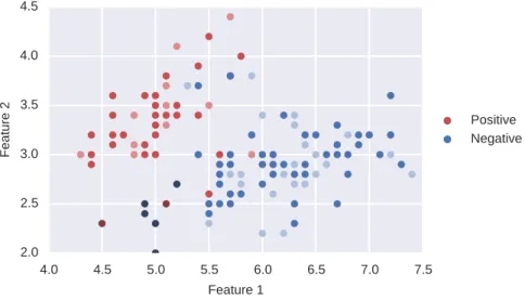
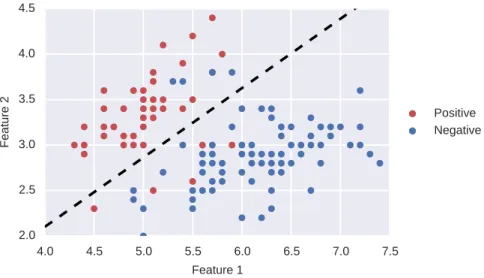
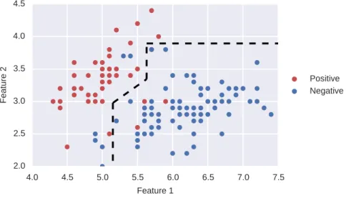
Figure2.2: Example of a classification algorithm. Using a set of examples from two classes, a classification algorithm is learned in order to separate between the positives and the negatives.
Then the algorithm is used to estimate the classes c of a set of testing examplesStest.
There exists several algorithms that can be used for classification tasks. In general a classification algorithm is learned with the objective of find-ing patterns that separate between the different classes [Hastie et al., 2009]. In order to clarify this intuition, in Figure2.2an example of a clas-sification algorithm is shown. Let us consider a set of examples, where the red points represent the positive examples and the blue ones the negative examples. The objective of a classifier is to find the best way to separate between the positive and negative examples. Then, the output of a classifier learned using the set of training examples is shown as the dashed black line. It is observed that this classifier is able to separate almost all the examples using a linear classifier. However, not all amples are correctly classified. In particular, there are four negative ex-amples that were predicted as positive, and five positive exex-amples that were predicted as negative. In the next section, we present the standard methods for evaluating the performance of a classification algorithm.
2.2 t r a d i t i o na l e va l uat i o n m e a s u r e s
When evaluating the performance of a classification algorithm, the first thing to do is to check the number of examples that were misclassified, since the true class of the examples is known. Therefore, evaluating
12 b a s i c s o n c l a s s i f i c at i o n
Actual Positive Actual Negative
yi=1 yi =0
Predicted Positive
True Positive (T P) False Positive (FP)
ci =1
Predicted Negative
False Negative (FN) True Negative (T N)
ci =0
Table2.1: Classification confusion matrix
the error of a model is as simple as counting the number of times an example is misclassified divided by the number of examples
Err(f(S)) =1− 1 N N X i=1 1yi(ci), (2.2)
where1q(z) is an indicator function that is calculated as:
1q(z) = 1 if z =q 0 if z 6=q. (2.3)
Moreover the accuracy is defined as the percentage of times the algo-rithm made the correct prediction
Acc(f(S)) =1−Err(f(S)). (2.4)
However, just knowing these statistics is not enough to make deci-sions, as in many applications it is important to know where the errors are coming from. In particular, the misclassified examples may belong only to one class, which may give interesting insights about the prob-lem. A way to observe the different errors is by looking at the confusion matrix, as shown in Table2.1. Afterwards, using the cost matrix several statistics are extracted. In particular:
Recall= T P
T P+FN (2.5)
Precision= T P
T P+FP (2.6)
F1Score=2 Precision·Recall
2.2 t r a d i t i o na l e va l uat i o n m e a s u r e s 13 4.0 4.5 5.0 5.5 6.0 6.5 7.0 7.5 Feature 1 2.0 2.5 3.0 3.5 4.0 4.5 Fe at ure 2 Positive Negative
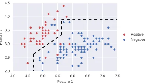
Figure2.3: Example of a classification algorithm. Using a set of examples from two classes, a classification algorithm is learned in order to separate between the positives and the negatives.
As an illustrative example, the different statistics are calculated for the example presented in Section 2.1. First, the confusion matrix is cal-culated as follows:
Actual Positive Actual Negative
yi=1 yi=0 Predicted Positive 36 4 ci=1 Predicted Negative 5 68 ci=0
Then using the confusion matrix, the different statistics are calculated as: Error =11.11%, Recall =87.8%, Precision =90% andF1Score=88.8%.
There are, however, several instances that are misclassified, that is be-cause the simple linear classifier that was used in this example may not be good enough to separate between the positive and negative classes. In order to make a comparison, using the same example, a new algo-rithm is learned. This time the algoalgo-rithm made the correct prediction more often as shown in Figure2.3. Afterwards, the confusion matrix is calculated as follows:
Actual Positive Actual Negative
yi=1 yi=0 Predicted Positive 37 2 ci=1 Predicted Negative 4 70 ci=0
14 b a s i c s o n c l a s s i f i c at i o n
Then the different statistics are calculated as: Error = 5.3%, Recall = 90.2%, Precision = 94.9% and F1Score = 92.5%. It is observed that in
this case the FP are reduced more than the FN, this leads to a higher increase in precision than in recall. There is not a single rule regarding which one is more important than the other, it depends on the applica-tion. For example in applications with a high false negative cost such as failing to identify a tumor in a medical exam, the recall should be the priority, even if that implies having a significant number of false positives. On the other hand, In applications such as spam detection, predicting a normal email as spam it may have a large impact on the customer, therefore, in this example is better to allow some false nega-tives and focus on the false posinega-tives.
It is not always straightforward to define the right tradeoff between false positives and false negatives. The best approximation to solve that, is to focus on the actual costs incurred by the different decisions. This is usually solved using cost-sensitive classification methods.
2.2.1 Brier score
Traditional evaluation measures of binary classification problems, such as Accuracy and F1Score, provide a way to analyze the performance of
a model. However, when using the classifier output as a basis for deci-sion making, there is a need of a measure that takes into account not only the misclassification of a classifier predicted class c, but also the quality of the estimated probabilities ˆp [Cohen and Goldszmidt, 2004]. The most appropriate is the Brier score [Brier, 1950]. The Brier score belongs to the class of so-called proper scores which are used in evalu-ating the subjective probability assessment of the prediction [DeGroot and Fienberg, 1983]. The Brier score is the average squared difference between the estimated probability and the true class label. It is defined as: BS(f(S)) = 1 N N X i=1 (pˆi−yi)2. (2.8)
The main justification of this score is based on decision theoretic con-siderations, in the sense that, a forecaster should pay a price propor-tional to the confidence with which it asserts its decision.
3
C O S T - S E N S I T I V E C L A S S I F I C AT I O N
Outline
In this chapter, we introduce the problem of cost-sensitive classifica-tion. Standard classification models aim at minimizing the misclassifica-tion of examples, in which an example is misclassified if the predicted class is different from the true class. However, this is not the case in many real-world applications. In this chapter, first, we introduce cost-sensitive classification in Section 3.1. Then, in Section 3.2, we present the problem of class-dependent cost-sensitive classification. Then, in Section 3.3, we present the general framework of example-dependent cost-sensitive classification. Within this section, we first introduce a method for defining the type of cost-sensitivity of a problem. After-wards, we present the different cost-sensitive performance evaluation measures. Lastly, we present state-of-the-art example-dependent cost-sensitive methods, namely, cost-proportionate rejection-sampling and cost-proportionate over-sampling.
3.1 i n t r o d u c t i o n
Classification methods are used to predict the class of different exam-ples given their features. Standard methods aim at maximizing the accu-racy of the predictions, in which an example is correctly classified if the predicted class is the same the as true class. This traditional approach assumes that all correctly classified and misclassified examples carry the same cost. This, however, is not the case in many real-world appli-cations. Methods that use different misclassification costs are known as cost-sensitive classifiers. Typical cost-sensitive approaches assume a con-stant cost for each type of error, in the sense that, the cost depends on the class and is the same among examples [Elkan,2001;Kim et al.,2012]. Nevertheless, this class-dependent approach is not realistic in many real-world applications.
For example in credit card fraud detection, failing to detect a fraud-ulent transaction may have an economical impact from a few to thou-sands of Euros, depending on the particular transaction and card holder [Sahin et al., 2013]. In churn modeling, a model is used for predicting which customers are more likely to abandon a service provider. In this context, failing to identify a profitable or unprofitable churner has a sig-nificant different financial impact [Glady et al.,2009]. Similarly, in direct
16 c o s t-s e n s i t i v e c l a s s i f i c at i o n
marketing, wrongly predicting that a customer will not accept an offer when in fact he will, has a different impact than the other way around [Zadrozny et al., 2003]. Also in credit scoring, where declining good customers has a non constant impact since not all customers generate the same profit [Verbraken et al., 2014]. Lastly, in the case of intrusion detection, classifying a benign connection as malicious has a different cost than when a malicious connection is accepted [Ma et al., 2011].
In order to deal with these specific types of cost-sensitive problems, called example-dependent cost-sensitive, some methods have been pro-posed recently. However, the literature on example-dependent cost-sensitive methods is limited, mostly because there is a lack of publicly available datasets that fit the problem [Aodha and Brostow, 2013]. Stan-dard solutions consist in modifying the training set by re-weighting the examples proportionately to the misclassification costs [Elkan, 2001; Zadrozny et al.,2003].
3.2 c l a s s-d e p e n d e n t c o s t-s e n s i t i v e c l a s s i f i c at i o n
The literature in cost-sensitive classification is mostly focused in class-dependent problems [Elkan,2001], where the cost of misclassification is associated with the class. Usually, the cost of misclassifying a positive example is denoted by CFNand the one of misclassifying a negative
ex-ample is denoted byCFP. Conceptually,CFN >0andCFP >0; moreover,
they are normally defined such that CFN+CFP = 2 [Flach et al., 2011],
as when CFN = CFP = 1 represents the case of cost-insensitive
classifi-cation. Using the previous notation, a class-dependent cost measure is defined as [Wang et al.,2014]:
Costcd(f(S)) =CFP·FP+CFN·FN. (3.1)
Over the past decades, various algorithms have been proposed for class-dependent cost-sensitive classification in literature. Several au-thors have used modifications of the decision trees that take into ac-count the different class-dependent costs [Draper et al.,1994;Ting,2002; Ling et al.,2004;Li et al.,2005;Kretowski and Grze´s,2006;Vadera,2010; Lomax and Vadera, 2013]. Similarly, applications of bagging and boost-ing algorithms have been used for cost-sensitive classification [Nesbitt, 2010; Street, 2008; Masnadi-shirazi and Vasconcelos, 2011; Fan et al., 1999]. Recently, various variations to support vector machines have also been used for this problem [Li et al.,2010;Masnadi-shirazi,2010]. Lastly, online learning algorithms have also been used for cost-sensitive tasks [Wang et al., 2014].
Following the example shown in Section 2.1, we now assume that misclassifying a negative example has a cost ofCFN =0.2and for a
pos-3.3 e x a m p l e-d e p e n d e n t c o s t-s e n s i t i v e c l a s s i f i c at i o n 17 4.0 4.5 5.0 5.5 6.0 6.5 7.0 7.5 Feature 1 2.0 2.5 3.0 3.5 4.0 4.5 Fe at ure 2 Positive Negative
Figure3.1: Class-dependent cost-sensitive classification algorithm. Since the cost of misclassifying positives and negatives is different, the algo-rithm focus on maximizing the correct classification of the positives.
itive example, the cost isCFP =1.8. Under this scenario, misclassifying a positive example has a much higher cost than misclassifying a negative one. Taking that into account, in Figure 3.1, we show an algorithm (Al-gorithm3), that focused on maximizing the correct classification of the
positives. In the following table, we compare the results of the standard measures and the class-dependent cost, of Algorithm3 and the
classifi-cation algorithms presented in Figure 2.2 (Algorithm1) and Figure 2.3 (Algorithm2):
Algorithm Error Recall Precision F1Score Costcd
Algorithm1 11.11% 87.8% 90% 88.8% 9.8
Algorithm2 5.3% 90.2% 94.9% 92.5% 7.6
Algorithm3 7.97% 92.68% 86.36% 89.41% 6.6
It is found, that by focusing on the positives, Algorithm3 arises to
a lower cost, even though the traditional metrics are worse for Algo-rithm3 than for Algorithm2. In conclusion, it is of highly importance to
take into account the cost when evaluating and training a classification model.
3.3 e x a m p l e-d e p e n d e n t c o s t-s e n s i t i v e c l a s s i f i c at i o n
The class-dependent framework introduced in the previous section is highly restrictive, as assuming that the different costs are constant be-tween classes is not realistic in many real world applications. In fraud detection, fraudulent transactions can have a financial impact from
hun-18 c o s t-s e n s i t i v e c l a s s i f i c at i o n
Actual Positive Actual Negative
yi=1 yi=0 Predicted Positive CT Pi CFPi ci=1 Predicted Negative CFNi CT Ni ci=0
Table3.1: Classification cost matrix
Negative C∗FN i= (CFNi−CT Ni) (CFPi−CT Ni) Positive C∗T P i = (CT Pi−CT Ni) (CFPi−CT Ni)
Table3.2: Simplified classification cost matrix [Elkan,2001]
dreds or thousands of Euros [Sahin et al., 2013]. In this context, the example-dependent costs can be represented using a 2x2 cost matrix
[Elkan,2001], that introduces the costs associated with two types of cor-rect classification, cost of true positives (CT Pi), cost of true negatives (CT Ni), and the two types of misclassification errors, cost of false posi-tives (CFPi), cost of false negatives (CFNi), as defined in Table3.1.
Conceptually, the cost of correct classification should always be lower than the cost of misclassification. These are referred to as the “reason-ableness“ conditions [Elkan,2001], and are defined as CFP
i > CT Ni and CFNi > CT Pi. Taking into account the “reasonableness“ conditions, a simpler cost matrix with only one degree of freedom has been defined in [Elkan,2001], by scaling and shifting the initial cost matrix. The sim-pler cost-matrix is shown in Table 3.2.
3.3.1 Example-dependent evaluation measures
Common cost-insensitive evaluation measures, such as misclassification rate orF1Score, assume the same cost for the different misclassification errors. Using these measures is not suitable for example-dependent cost-sensitive binary classification problems. Indeed, two classifiers with equal misclassification rates but different numbers of false positives and false negatives do not have the same impact on cost since CFPi 6=CFNi; therefore, there is a need for a measure that takes into account the ac-tual costs {CT Pi,CFPi,CFNi,CT Ni} of each example i, as introduced in Section3.3.
Let Sbe a set of Nexamplesi, N= |S|, where each example is
3.3 e x a m p l e-d e p e n d e n t c o s t-s e n s i t i v e c l a s s i f i c at i o n 19
and labeled using the class label yi ∈ {0,1}. A classifier fwhich
gener-ates the predicted label ci for each element i is trained using the set S. Then the cost of using fonSis calculated by
Cost(f(S)) = N X i=1 Cost(f(x∗i)), (3.2) where Cost(f(x∗i)) =yi(ciCT Pi+ (1−ci)CFNi)+ (1−yi)(ciCFPi+ (1−ci)CT Ni). (3.3)
However, the total cost may not be easy to interpret. In [Whitrow et al., 2008], anormalizedcost measure was proposed, by dividing the total cost by the theoretical maximum cost, which is the cost of misclassifying every example. Thenormalizedcost is calculated using
Costn(f(S)) =
Cost(f(S))
PN
i=1CFNi·10(yi) +CFPi·11(yi)
. (3.4)
We propose similar approach in [Correa Bahnsen et al.,2014a], where the savings of using an algorithm are defined as the cost of the algo-rithm versus the cost of using no algoalgo-rithm at all. To do that, the cost of the costless class is defined as
Costl(S) =min{Cost(f0(S)),Cost(f1(S))}, (3.5)
where
fa(S) ={a}, witha∈{0,1}. (3.6)
The cost improvement can be expressed as the cost savings as com-pared with Costl(S).
Savings(f(S)) = Costl(S) −Cost(f(S)) Costl(S)
. (3.7)
In order to illustrate this concept, we use the same example shown in Section2.1. However, now we add the variation in the costs by showing the examples with the highest cost darker, and the ones with the lowest cost lighter. The new example is shown in Figure 3.2. Moreover, in the following table we summarize the different example-dependent costs:
Class Cost light Cost normal Cost dark
Negative 0.1 0.5 5.0
20 c o s t-s e n s i t i v e c l a s s i f i c at i o n 4.0 4.5 5.0 5.5 6.0 6.5 7.0 7.5 Feature 1 2.0 2.5 3.0 3.5 4.0 4.5 Fe at ure 2 Positive Negative
Figure3.2: Example with example-dependent costs. Examples with the highest
cost in darker colors, and the ones with the lowest cost are in lighter colors. 4.0 4.5 5.0 5.5 6.0 6.5 7.0 7.5 Feature 1 2.0 2.5 3.0 3.5 4.0 4.5 Fe at ure 2 Positive Negative
Figure3.3: Example-dependent cost-sensitive classification algorithm. The al-gorithm focus first on correctly classify the dark examples, as the cost of misclassification in this cases is several times more expensive than the other cases.
Taking into account the example-dependent costs, in Figure 3.3 (Al-gorithm4), we show a new algorithm that gives a higher importance on
correctly classify the dark examples, as the cost of misclassification in this cases is several times more expensive than the other cases. Further-more, in the following table, we compare the results of the standard measures and the example-dependent savings of Algorithm4 and the
3.3 e x a m p l e-d e p e n d e n t c o s t-s e n s i t i v e c l a s s i f i c at i o n 21
classification algorithms presented in Figure 2.2 (Algorithm1), Figure
2.3 (Algorithm2) and Figure3.1(Algorithm3):
Algorithm Error Recall Precision F1Score Savings
Algorithm1 11.11% 87.8% 90% 88.8% 46.86%
Algorithm2 5.3% 90.2% 94.9% 92.5% 68.36%
Algorithm3 7.97% 92.68% 86.36% 89.41% 48.07%
Algorithm4 6.19% 92.68% 90.48% 91.56% 87.42%
With these examples, we illustrate the impact that the costs have on the algorithms. Moreover, we highlight the importance of using the dif-ferent costs when evaluating the difdif-ferent models. It is worth mention-ing how distinct are the results if the costs are ignored and an algo-rithm is trained and evaluated not taking into account the different costs present in most real-world applications.
3.3.2 Binary classification cost characteristic
A classification problem is said to be cost-insensitive if costs of both errors are equal. It is class-dependent cost-sensitive if the costs are dif-ferent but constant. Finally we talk about an example-dependent cost-sensitive classification problem if the cost matrix is not constant for all the examples.
However, the definition above is not general enough. There are many cases when the cost matrix is not constant and still the problem is cost-insensitive or class-dependent cost-sensitive. For example, if the costs of correct classification are zero, CT Pi = CT Ni = 0, and the costs of misclassification are CFPi = a0·zi and CFNi = a1·zi, where a0 and a1, are constants and zi is a random variable. This is an example of a
cost matrix that is not constant. However, C∗FN
i and C ∗ T Pi are constant, i.e. C∗FN i = (a1·zi)/(a0·zi) = a1/a0 and C ∗
T Pi = 0 ∀i. In this case the problem is cost-insensitive if a0 =a1, or class-dependent cost-sensitive ifa0 6=a1, even given the fact that the cost matrix is not constant.
Nevertheless, using only the simpler cost matrix is not enough to de-fine when a problem is example-dependent cost-sensitive. To achieve this, we defined the following cost characteristic for a given binary clas-sification problem as:
bi =C∗FNi−C ∗
T Pi, (3.8)
and define its mean and standard deviation asµband σb, respectively.
Usingµb and σb, we analyze different binary classification problems.
A binary classification problem is defined according to the following conditions:
22 c o s t-s e n s i t i v e c l a s s i f i c at i o n
µb σb Type of classification problem
1 0 cost-insensitive
6=1 0 class-dependent cost-sensitive
6=0 example-dependent cost-sensitive
3.3.3 State-of-the-art methods
As mentioned earlier, taking into account the different costs associated with each example, some methods have been proposed to make classi-fiers example-dependent cost-sensitive. These methods may be grouped in two categories. Methods based on changing the class distribution of the training data, which are known as cost-proportionate sampling methods; and direct cost methods [Wang, 2013].
A standard method to introduce example-dependent costs into classi-fication algorithms is to re-weight the training examples based on their costs, either by cost-proportionate rejection-sampling [Zadrozny et al., 2003], or over-sampling [Elkan,2001]. The rejection-sampling approach consists in selecting a random subset Sr by randomly selecting
exam-ples fromS, and accepting each exampleiwith probabilitywi/max 1,...,N{wi},
wherewi is defined as the expected misclassification error of examplei:
wi =yi·CFNi+ (1−yi)·CFPi. (3.9)
Lastly, the over-sampling method consists in creating a new set So, by
making wi copies of each examplei. However, cost-proportionate
over-sampling increases the training since|So| >> |S|, and it also may result
in over-fitting [Drummond and Holte,2003]. Furthermore, none of these methods uses the full cost matrix but only the misclassification costs.
The second approach consists in using the predicted probability ˆpi,
estimated using a given classifier f, and modify the threshold t such that the savings are maximized. This method is called cost-sensitive thresholding [Sheng and Ling, 2006]. The idea behind this approach is to adaptively modify the probability threshold of an algorithm ft in order to maximize the savings Savings(ft(S)) of the algorithm ft on a given setS. The threshold is calculated using the following equation
tthresholding =arg max
t
Part II
R E A L - W O R L D E X A M P L E - D E P E N D E N T
A P P L I C AT I O N S
4
F I N A N C I A L R I S K M O D E L I N G
Outline
In this chapter, we present two different real-world example-dependent cost-sensitive problems related to financial risk modeling, namely, credit card fraud detection and credit scoring. Both problems are example-dependent cost-sensitive, as failing to identify a fraudulent transaction may have a financial impact ranging from tens to thousands of Euros. Similarly, in credit scoring, approving a customer that later does not pay his debt has a significant impact on a bank profit. First, in Section 4.1, we introduce the credit card fraud detection problem and propose new periodic features. Lastly, in Section 4.2, we present the credit scoring problem and propose a new financial evaluation measure for this prob-lem.
4.1 c r e d i t c a r d f r au d d e t e c t i o n
The use of credit and debit cards has increased significantly in the last years, unfortunately so has the fraud. Because of that, billions of Eu-ros are lost every year. According to the European Central Bank [Euro-pean Central Bank, 2014], during 2012 the total level of fraud reached 1.33 billion Euros in the Single Euro Payments Area, which represents
an increase of 14.8% compared with 2011. Moreover, payments across
non traditional channels (mobile, internet, ...) accounted for60% of the
fraud, whereas it was 46% in 2008. This opens new challenges as new
fraud patterns emerge, and current fraud detection systems are not be-ing successful in preventbe-ing fraud. Furthermore, fraudsters constantly change their strategies to avoid being detected, something that makes traditional fraud detection tools such as expert rules inadequate.
The use of machine learning in fraud detection has been an interest-ing topic in recent years. Several detection systems based on machine learning techniques have been successfully used for this problem [Bhat-tacharyya et al., 2011]. When constructing a credit card fraud detec-tion model, there are several problems that have an important impact during the training phase: Skewness of the data, cost-sensitivity of the application, short time response of the system, dimensionality of the search space and how to preprocess the features [Bolton et al., 2002; Bachmayer, 2008; Whitrow et al., 2008; Pozzolo et al., 2014a; Van
26 f i na n c i a l r i s k m o d e l i n g
selaer et al., 2015]. We are interested in addressing the cost-sensitivity and the features preprocessing issues.
Credit card fraud detection is by definition a cost-sensitive problem, in the sense that the cost due to a false positive is different than the cost of a false negative. When predicting a transaction as fraudulent, when in fact it is not a fraud, there is an administrative cost that is incurred by the financial institution. On the other hand, when failing to detect a fraud, the amount of that transaction is lost [Hand et al., 2007]. Moreover, it is not enough to assume a constant cost difference between false positives and false negatives, as the amount of the transactions varies quite significantly; therefore, its financial impact is not constant but depends on each transaction.
When constructing a credit card fraud detection model, it is very im-portant to use those features that will help the algorithm make the best decision. Typical models only use raw transactional features, such as time, amount, place of the transaction. However, these approaches do not take into account the spending behavior of the customer, which is expected to help discover fraud patterns [Bachmayer, 2008]. A stan-dard way to include these behavioral spending patters was proposed in [Whitrow et al., 2008], where Whitrow et al. proposed a transaction aggregation strategy in order to take into account a customer spending behavior. The derivation of the aggregated features consists in group-ing the transactions made durgroup-ing the last given number of hours, first by card or account number, then by transaction type, merchant group, country or other, followed by calculating the number of transactions or the total amount spent on those transactions.
In this section, we first present a new cost-based measure to evaluate credit card fraud detection models, taking into account the different fi-nancial costs incurred by the fraud detection process. Afterwards, we propose an expanded version of the transaction aggregation strategy, by incorporating a combination criteria when grouping transactions, i.e., instead of aggregating only by card holder and transaction type, we combine it with country or merchant group. This allows to have a much richer feature space. Moreover, we are interested in analyzing the impact of adding the time of a transaction. The logic behind it, is that a customer is expected to make transactions at similar hours. We, hence, propose a new method for creating features based on the peri-odic behavior of a transaction time, using the von Mises distribution [Fisher, 1996]. In particular, these new time features should estimate if the time of a new transaction is within the confidence interval of the previous transaction time. Furthermore, we present the real credit card fraud dataset provided by a large European card processing company used for the experiments in this thesis.
4.1 c r e d i t c a r d f r au d d e t e c t i o n 27
4.1.1 Credit card fraud detection evaluation
A credit card fraud detection algorithm consists in identifying those transactions with a high probability of being fraud, based on histor-ical fraud patterns. The use of machine learning in fraud detection has been an interesting topic in recent years. Different detection sys-tems that are based on machine learning techniques have been success-fully used for this problem, in particular: neural networks [Maes et al., 2002], Bayesian learning [Maes et al., 2002], artificial immune systems [Bachmayer, 2008], association rules [Sánchez et al., 2009], hybrid mod-els [Krivko, 2010], support vector machines [Bhattacharyya et al., 2011], peer group analysis [Weston et al.,2008], online learning [Pozzolo et al., 2014a], discriminant analysis [Mahmoudi and Duman,2015] and social network analysis [Van Vlasselaer et al.,2015].
Most of these studies compare their proposed algorithm with a bench-mark algorithms and then make the comparison using a standard binary classification measure, such as misclassification error, receiver operating characteristic (ROC), Kolmogorov-Smirnov (KS) or F1Score statistics [Bolton et al., 2002; Hand et al., 2007; Pozzolo et al., 2014a]. However, these measures may be not the most appropriate evaluation criteria when evaluating fraud detection models, because they tacitly assume that misclassification errors carry the same cost, similarly with the correct classified transactions. This assumption does not hold in practice, since wrongly predicting a fraudulent transaction as legitimate carries a significantly different financial cost than the inverse case. Fur-thermore, the accuracy measure also assumes that the class distribution among transactions is constant and balanced [Provost et al., 1998], and typically the distributions of a fraud detection dataset are skewed, with a percentage of frauds ranging from 0.005% to 0.5% [Bachmayer, 2008; Bhattacharyya et al.,2011].
In order to take into account the different costs of fraud detection during the evaluation of an algorithm, we may use the cost matrix de-fined in Table3.1. Hand et al. [Hand et al.,2007] proposed a cost matrix, where in the case of false positive the associated cost is the adminis-trative cost CFPi = Ca related to analyzing the transaction and con-tacting the card holder. This cost is the same assigned to a true positive CT Pi =Ca, because in this case, the card holder will have to be contacted. However, in the case of a false negative, in which a fraud is not detected, the cost is defined to be a hundred times larger, i.e.CFNi =100Ca. This same approach was also used in [Bachmayer, 2008].
Nevertheless, in practice, losses due to a specific fraud range from few to thousands of Euros, which means that assuming constant cost for false negatives is unrealistic. In order to address this limitation, we
pro-28 f i na n c i a l r i s k m o d e l i n g
Actual Positive Actual Negative
yi=1 yi=0 Predicted Positive C T Pi =Ca CFPi =Ca ci=1 Predicted Negative CFNi =Amti CT Ni=0 ci=0
Table4.1: Credit card fraud cost matrix
pose a cost matrix that takes into account the actual example-dependent financial costs. Our cost matrix defines the cost of a false negative to be the amount CFNi = Amti of the transaction i. We argue that this cost matrix is a better representation of the actual costs, since when a fraud is not detected, the losses of that particular fraud correspond to the stolen amount. The costs are summarized in Table4.1.
Afterwards, using (3.3) a cost measure for fraud detection is calcu-lated as: Cost(f(S)) = N X i=1 yi(1−ci)Amti+ciCa, (4.1)
then, the savings of an algorithm are calculated using (3.7).
4.1.2 Feature engineering for fraud detection
When constructing a credit card fraud detection algorithm, the initial set of features (raw features) include information regarding individual transactions. It is observed throughout the literature, that regardless of the study, the set of raw features is quite similar. This is because the data collected during a credit card transaction must comply with international financial reporting standards [American Institute of CPAs, 2011]. In Table 4.2, the typical credit card fraud detection raw features are summarized.
4.1.2.1 Customer spending patterns
Several studies use only the raw features in carrying their analysis [Brause et al., 1999; Minegishi and Niimi, 2011; Panigrahi et al., 2009; Sánchez et al., 2009]. However, as noted in [Bolton and Hand, 2001], a single transaction information is not sufficient to detect a fraudulent transaction, since using only the raw features leaves behind important information such as the consumer spending behavior, which is usually used by commercial fraud detection systems [Whitrow et al., 2008].
![Table 3.2: Simplified classification cost matrix [Elkan, 2001 ]](https://thumb-us.123doks.com/thumbv2/123dok_us/9736599.2464664/40.892.249.643.104.396/table-simplified-classification-cost-matrix-elkan.webp)