Alternative Trajectory Options for Delay Reduction
in Demand and Capacity Balancing
Yan Xu, Ramon Dalmau, Marc Melgosa, Adeline Montlaur, Xavier Prats
Department of Physics - Aeronautics DivisionTechnical University of Catalonia Castelldefels 08860, Barcelona (Spain)
Abstract—Aiming to a more collaborative demand and capac-ity balancing (DCB), in the scope of trajectory based operations, this paper presents an approach that takes alternative trajectories into a DCB optimization algorithm. These alternative trajectories are generated by the airspace users for those flights traversing hotspots (i.e. sectors with demand above capacity), which are predicted by the Network Manager. The trajectories consider lateral re-routings and/or vertical avoidance of all detected hotspots, which, along with different types of delay measures (including linear holding and in-flight delay recovery), are then integrated as a whole into a centralized optimization model to manage the traffic flow under a set of static scheme of airspace capacities. The combination of trajectory options and distribution of delays are hence optimized with the objective of minimizing the total deviation with regard to airspace users’ preferences (taking into account the fuel consumption, route charge and the cost of delay). Results suggest that delays can be remarkably reduced once alternative trajectory options are included in the DCB algorithm. Nevertheless, this delay reduction is obtained by diverting a large number of flights, yielding to an interesting trade-off between environmental impact and cost-efficiency for the airspace users.
NOMENCLATURE
f∈F set of flights
k∈Kf set of submitted trajectories for flightf j∈Pk set of elementary sectors thatktraverses
t∈T set of time moments
τ ∈ T set of time periods for unit capacity
l∈Sjτ set of collapsed sectors includingj inτ P(k, i)
the departure airport, ifi= 1
the arrival airport, ifi=nf
sector positions, if1< i < nf rjk the estimated time over ofkatj
Tkj [rjk, rjk+ejk], the feasible time window fork atj zkj,j0 rjk0−rkj:P(k, i) =j,P(k, i+ 1) =j0, the
estimated time over of two contiguous positions
uj,jk 0 the delay recovery bound of contiguous positions
vkj,j0 the linear holding bound of contiguous positions The work presented in this paper was partially funded by grants from the Funds of China Scholarship Council (201506830050) and by the SESAR Joint Undertaking under grant agreement No 699338, as part of the European Unions Horizon 2020 research and innovation programme: APACHE project (Assessment of Performance in current ATM operations and of new Concepts of operations for its Holistic Enhancement - http://apache-sesar.barcelonatech-upc.eu/en). The opinions expressed herein reflect the authors view only. Under no circumstances shall the SESAR Joint Undertaking be responsible for any use that may be made of the information contained herein.
S(k, l, τ) the first entered elementary sector forkamong those collapsed intol inτ
CjD(τ) the airport departure capacity inτ CA
j(τ) the airport arrival capacity inτ
ClS(τ) the sector capacity of operating sectorlinτ
I. INTRODUCTION
Airports and airspace sectors are both limited in capacity by operational constraints [1]. Severe weather, such as convective weather, can significantly reduce these capacities producing imbalance between capacity and demand and subsequent air traffic disruptions and delays. In order to regulate the traffic flow when demand is expected to exceed capacity, Traffic Management Initiatives (TMI) are implemented. Examples of these regulations in the United States are Ground delay Pro-grams (GDPs) and Airspace Flow ProPro-grams (AFPs). Similar initiatives exist in Europe and in other regions of the world where ATFM (air traffic flow management) is deployed. GDPs control the arrival rate at an affected airport by assigning departure delays to flights at their origin airports. Similarly, an AFP identifies constraints in the en-route system, regulating flights filed into the Flow Constrained Area (FCA) [2]. While a flight has no choice but to eventually end up at its destination airport, a capacity-constrained en-route sector can often be bypassed at limited cost by selecting an alternative route. To that aim, AFPs specify available reroutes that avoid the FCA. Flight operators may then choose to accept the delay for an affected flight, or to take the available reroute [3].
The overall objective of TMI is typically to reach a global optimum (e.g., minimize total delay across all controlled flights) based on some unanimous fairness criteria (e.g., first scheduled, first served), but not takes into account specific preferences of a particular flight, in line to the airspace user cost model. However, the paradigm change for the future air traffic management (ATM), proposed by SESAR (Single European Sky ATM Research) in Europe and NextGen (Next Generation Air Transportation System) in the United States, has aimed to shift from airspace based operations to trajec-tory based operations (TBO). In this context, airspace user involvement and flexibility in route selection are made possible thanks to Collaborative Decision Making (CDM) initiatives [4]. Under current GDPs, one of the most sophisticated ATFM tools used in the United States, resources (i.e., arrival slots)
are assigned to flights in accordance with a ration-by-schedule (RBS) mechanism. It is complemented by CDM initiatives, such as flight substitution, cancellations, compression, or slot credit substitution, allowing airlines to manage their own flights in line with their specified policies [5].
Increased CDM is found in the Collaborative Trajectory Options Program (CTOP), a recent TMI built upon concepts found in GDPs and AFPs, which consists in managing demand through constrained airspace. A new concept in the CTOP is that airspace users are able to communicate their preferences, with regard to both route and delay, in a trajectory options set [6]. Current version of CTOP implements an RBS scheme, that is, flights are assigned the best available routes and slots available at the time flight operators submit their preference requests during the planning period, in a sequential manner [7]. Recently, an alternative flight scheduling approach based on linear optimization instead of RBS has been studied, whilst using a Max-Min fairness rule to maintain the equity [8].
In this paper, we present a collaborative demand and ca-pacity balancing (CDCB) algorithm, closely related to the principle of CTOP, in the scope of full trajectory based operations. The main contributions of this model include: 1) instead of using experience-based alternative trajectories submitted by airspace users, we enable the hotspot-oriented avoidance information to be issued in such a way that airspace users could accurately design their own alternative trajectory based on short-term predicted situations (with as few extra cost as possible); and 2) more measures become available to manage the traffic flow in a higher flexible and cost-efficient way, and are integrated into an optimization model. They are composed of three trajectory options and four types of delay management strategies (including linear holding and in-flight delay recovery), which can be further mixed to a maximum of 45 different combinations to solve a given demand and capacity imbalance problem for each flight.
II. TRAJECTORY SUBMISSION PROCESS
This section introduces a primary trajectory submission process. Time-dependent hotspots are detected in pre-tactical phase (i.e., typically 1 day to 6 days before the day of operations), using airspace users’ initial trajectories, based on which the avoidance information is given to individual flights that are captured. In this way, accurate alternative trajectories (along with delay management preferences) can be generated to avoid the hotspots, with minimum extra costs.
A. Initial trajectory scheduling
The initial trajectory scheduling contains both lateral route planning and vertical profile optimization. An integrated model producing both at the same time will achieve the absolute opti-mal trajectory, but may also heavily increase the computational burden. In this paper, to simplify the problem for every single flight among a large amount of simulations, the lateral route will be first determined, followed by generating the vertical profile on the fixed route.
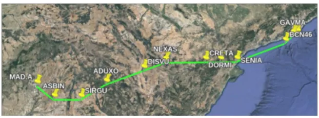
Fig. 1. Lateral route along structured flight segment with minimal costs
For planning the lateral route, we adopt the widely-used A* algorithm (which is a modification of Dijkstra’s Algorithm [9] specifically for a single destination) to compute the cheapest path that is connected by various route segments, as shown in Fig. 1. The weighted costs include fuel consumption (affected by distance flown and wind effects) and ANSP (Air Navigation Service Provider) route charges that might differ for different airspaces (see their effects on European route choices in [10]). For the heuristic part, the straight distance from the current node (i.e., ending point of a route segment) to the destination airport is considered.
On the other hand, the optimization of vertical profile re-quires the definition of a mathematical model representing air-craft dynamics and performances, along with a model for cap-turing certain atmospheric parameters. A generic vertical tra-jectory can be partitioned into several phasesi∈ {1,· · ·, N}, where different constraints may apply, as shown in Fig. 2. The objective function of the vertical profile optimization in this paper is to minimize a compound cost function J over the whole time window [t(1)0 , t(fN)]as follows:
J =
Z t(fN)
t(1)0
(F F(t) +CI)dt (1) where F F(t) is the fuel flow and CI is the Cost Index, combined to reflect airspace users’ direct operating costs.
As this paper is aimed at the pre-tactical operation phase, the details of initial trajectory scheduling (as typically done in the strategic phase) are out of the scope of this paper. For more detailed methodology and techniques implemented in the regard of initial trajectory scheduling, the reader may direct to [11], [12].
B. Avoidance information for individual flight
To assist airspace users accurately design alternative tra-jectories for their affected flights, some specific avoidance information will be generated and shared to certain flights. Under the trajectory based operations, it is clear that not only the sector capacity changes with time (due to different sector configurations at different times for instance), but also the flight entry which is dependent on the timeline of a trajectory. The sectors used to define entry points are elementary sectors, because their geographical positions are fixed during a relatively long time. However, an elementary sector could be collapsed, in real operations, with other adjacent elementary sector(s), and becomes an operating sector at a certain time. As illustrated in Fig. 3, for a collapsed sector containing several elementary sectors, only the first entered elementary sector (where an entry point is defined) for the flight should be counted as one traffic demand of that operating sector, and the rest entires (in the same collapsed sector) will be regarded as internal movement.
With the time-associated hotspots defined, we capture the certain flights traversing those areas at the corresponding times, based on their initial trajectories; prepare for the avoidance information using sectors’ structure data and tra-jectory/sector intersection data; and eventually share this in-formation to each individual flight that is captured.
An example is presented in Table I for a specific flight. The main information for lateral-avoidance includes all the boundary points’ geographical positions, while for vertical-avoidance it tells the flight at which distance (to destination airport) it should start to change the initially scheduled altitude and at which distance to recover that altitude (if needed), as well as the non-selectable flight levels between the two distances, for each sector that the flight needs to avoid.
(a) Flight entry (red star intersection) counted
(b) Flight entry (red star intersection) not counted
Fig. 3. Count flight entry (intersection of trajectory with elementary sector) as traffic demand in a collapsed operating sector.
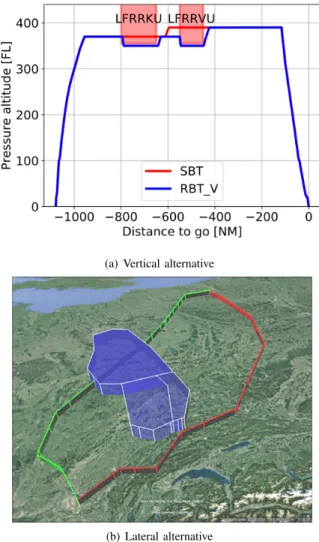
(a) Vertical alternative
(b) Lateral alternative
Fig. 4. Lateral- and vertical-avoidance alternative trajectories
C. Alternative trajectories and delay management
With the above avoidance information received, airspace users could easily re-design the optimal trajectory (i.e., alterna-tive trajectory) for each of their affected flights, using the same method as mentioned in Sec.II-A. The difference, compared to the initial trajectory, would be that more constraints have to be included in the trajectory optimization problem, in such a way that the re-designed trajectory will still be the optimal whilst being able to avoid the specified hotspots.
The lateral-avoidance case is shown in Fig. 4(b), where the additional constraints included to the lateral route planning should enforce that no intersection exists between the new trajectory and the frontier connected by any two adjacent boundary points (see Table I). The vertical-avoidance case shown in Fig. 4(a), should add to the vertical profile optimiza-tion with the extra constraints as already presented clearly by the avoidance information.
It must be noted that producing the new (alternative) tra-jectories does not mean that it will replace the initial one. Conversely, all will be taken into the model, and one of them will be eventually selected depending on the global optimum.
TABLE I
AVOIDANCE INFORMATION SHARED TO A PARTICULAR FLIGHT THAT IS INQUIRED TO PROVIDE ALTERNATIVE TRAJECTORIES.
Moreover, the production of alternative trajectories should not be mandatory, while airspace users could weigh the extra costs and make the decision according to their own situations.
Besides alternative trajectories, we also consider delays to manage the traffic flow. Different types of measures could be taken to absorb (or recover) the assigned delays, but the costs, limitations, and implementations of these measures are not necessarily the same. In this paper, four different measures are used including: ground holding, airborne holding, linear holding and delay recovery.
These delay measures will change the controlled times over along a 4-Dimensional trajectory. Typical airborne holding would consume more fuel due to the extended flight track, whilst ground holding has no impact in fuel consumption. Due to the increased extra fuel, the airborne holding time is fairly limited, taking account that safety related issues may arise from a reduction of the on-board reserve fuel. Ground holding can only be performed at the departure airport, prior to take-off. Airborne holding (including holding patterns or path stretching) can be done at any available airspace, in theory, but practically it is typically performed in designated locations.
Specifically, linear holding and delay recovery are also performed airborne, but rather than extending the flight path they will be realized following the original trajectory by means of a cost-based speed control. Generally, the amount of linear holding and delay recovery that can be achieved depends on several factors, such as the aircraft type, trip distance, payload, cruise flight level etc, as well as the extra fuel allowance (no extra fuel is also applicable for linear holding). This topic has been thoroughly discussed in [13], [14].
It is worth noting that for delay recovery, it is still aimed at the pre-tactical planning phase, obeying all the assigned controlled times along the trajectory. This should be differed from the tactical accelerating process under current operations where only the controlled time of departure (CTD) is enforced, rather than the controlled time of arrival (CTA) that is actually in effect. In addition, recall that the time-related costs have been already considered for initial trajectory scheduling (see Sec. II-A), which means the initial speed profile should be most preferred by airspace users. Hence, during the delay assignment process (as discussed in Sec. III), we allow delay recovery only if some delay is imposed at the forepart of a trajectory (such as ground holding at the origin airport).
III. DEMAND AND CAPACITY BALANCING
Sec. II has shown how the alternative trajectories are pro-duced, along with the basis of timeline preferences. Next, the following section is to take all these possible measures into account, which include three trajectory options (initial, lateral and vertical) and four delay management (ground holding, airborne holding, linear holding and delay recovery), to together balance the traffic demand and airspace capacity. A. Problem statement
To achieve the goal of demand and capacity balancing (DCB), improving the capacity via, e.g., dynamic sectorization based on specific traffic pattern or complexity (see for instance [15] and the references therein), is possible, but is out of the scope of this paper. In other words, the problem can be simplified as to manage the demand under a set of fixed capacity (for a static scheme of sector configurations). Two groups of decision variables are defined as follows:
(1) Decision variables for trajectory options:
wfk =
(
1, if trajectoryk is chosen for flightf 0, otherwise
(2) Decision variables for delay management:
xjk,t=
(
1, if trajectorykdeparts from positionj by timet 0, otherwise
yk,tj =
(
1, if trajectoryk arrives at position j by timet 0, otherwise
Note that the “by” time is used, rather than “at” to be the decision variables in this paper, which would enable a faster solution time according to [16], while the “at” time can be derived by (xjf,t−xjf,t−1) and (yjf,t−yjf,t−1) respectively.
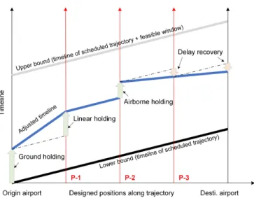
Fig. 5 shows schematically the trajectory timeline versus de-signed positions (i.e., intersection with elementary sectors) and the four types of delay management measures. An alternative trajectory means a new set of intermediate designed positions (e.g., P-1, P-2 and P-3). Ground holding is experienced only at the origin airport; airborne holding can only be performed “at” a given position (the difference between the “departure” and “arrival” time at that position equals to the holding time); and since linear holding and delay recovery are realized by
Fig. 5. Schematic of trajectory timeline versus designed positions.
speed control, the slope of the lines is increased or decreased if compared with the planned schedule.
B. Objective function
Recall that the initially scheduled trajectory should be the most preferred from an airspace user’s point of view, i.e., a local optimum. If all initial trajectories can be maintained in real execution, then the global optimum should be equal to the combination of all local optima. However, certain regulations might be invoked, such that the local optima cannot be all achieved. The objective function of this paper, therefore, min-imizes the total deviation from each local optimum, including the extra fuel consumption, extra route charges, and extra time related costs:
minJ = min(C∆F+C∆R+C∆T) (2) The extra fuel consumption C∆F can be represented as:
C∆F = X f∈F X k∈Kf αk·(T Jk−T Jf)·w f k (3)
whereT Jk andT Jf are respectively the total fuel consumed by trajectory k and by the initial trajectory of flight f. Note that k∈Kf, wherekis one of the trajectory options of flight f (Kf). Similarly, the extra route chargesC∆R are denoted:
C∆R= X f∈F X k∈Kf βk·(RCk−RCf)·wfk (4) Note that the route charges are calculated based on the absolute distance flown inside an area, rather than the straight distance between the entry and exit positions (and even not being charged for the extra distance due to tactical re-routings), as is for current operations.
The time-related costs are composed of those incurred from experiencing ground holding and air holding (includ-ing standard airborne hold(includ-ing and linear hold(includ-ing), as well
as performing delay recovery. Each coefficient is trajectory-dependent, which means that the values could be specified by airspace users for each individual trajectory1 For example, if one trajectory has high priority and requires as less delays as possible, then a greater value could be set toζk.
C∆T = X f∈F X k∈Kf [γk·GHk+δk·AHk−ζk·DRk] (5) With delay recoveryDRk =GHk+AHk−ADk, whereGHk is ground holding,AHk means air holding, andADk denotes arrival delay at the destination airport, we can organize Eq. 5:
C∆T = X f∈F X k∈Kf [(γk−ζk)·GHk+(δk−ζk)·AHk+ζk·ADk] (6) Specifically, GHk, AHk, and ADk can be respectively for-mulated by the decision variables as follows:
GHk= X t∈Tfj,P(f,1)=j (t−rjk)1+·(xjk,t−xjk,t−1) (7) AHk= X t∈Tkj,j∈P(k,i):1<i<nk t·(xjk,t−xjk,t−1−yjk,t+yk,tj −1) (8) ADk = X t∈Tkj,P(k,nk)=j (t−rkj)·(yk,tj −yk,tj −1) (9)
It must be noted that, although multiple collaboration proce-dures are conducted to obtain the input of the DCB problem, the above objective function is still of centralized nature (as it is for most existing ATFM initiatives). To realize a better collaborative effect in this regard, it could be appropriate to perform an iterative model execution process, allowing airspace users to revise, update, substitute or cancel their sub-mitted (alternative) trajectories based on the current assigned results. However, this process has not been included in this paper, where we only execute the model for once.
Besides, using the global cost across all the flights in the objective function is intended for achieving the highest system efficiency. The fairness issue, on the other hand, is out of the scope of this paper. In fact, the equilibrium criteria between different airspace users could be quite subjective, and, as reported by a number of studies, a strict fairness rule (e.g., first scheduled, first served) may trade for a significant reduction of efficiency. For such reasons, the fairness problem has been one of the main obstacles preventing various ATFM models to be implemented by practitioners. We believe that the same issue applies for the CDCB model as well, and it should deserve another subsequent work addressing in particular this problem.
1This may cause competition issues, such as potential gaming, which is still under assessment by the authors.
C. Constraints
The constraints of this model can be grouped into flight op-erations, user-specified limits, system capacities and decision variables, as presented in each subsection below.
X k∈Kf wkf = 1 ∀f ∈F (10) xj k,Tjk−1=y j k,Tjk−1= 0 ∀f ∈F,∀k∈Kf,∀j∈Pk (11) xj k,Tjk=y j k,Tjk=w f k ∀f ∈F,∀k∈Kf,∀j∈Pk (12) xjk,t−xjk,t−1≥0 ∀f ∈F,∀k∈Kf,∀j∈Pk,∀t∈Tkj (13) yk,tj −yk,tj −1≥0 ∀f ∈F,∀k∈Kf,∀j∈Pk,∀t∈Tkj (14) xjk,t−yk,tj ≤0 ∀f ∈F,∀k∈Kf,∀j∈Pk,∀t∈T j k (15) Constraint (10) enforces that one trajectory (initial or alter-native) is selected for each flight. Constraints (11)-(14) ensure that each selected trajectory k is assigned with only one slot for departing and arriving respectively at position j within the prescribed time window. Constraints (12) specifies that if a trajectory is not selected, then all the decision variables (including wfk,xjk,tandyjk,t) associated with it will be equal to zero. Constraint (15) states that the departure time is not earlier than arrival time at any position.
yj0 k,t+uj,jk 0·zkj,j0 −x j k,t≤0 ∀f ∈F,∀k∈Kf, ∀i∈[1, nk) :P(k, i) =j, P(k, i+ 1) =j0, ∀t∈Tkj∩(Tkj0−uj,jk 0·zj,jk 0) (16) xj k,t+vkj,j0·zkj,j0 −y j k,t≥0 ∀f ∈F,∀k∈Kf, ∀i∈[1, nk) :P(k, i) =j, P(k, i+ 1) =j0, ∀t∈Tkj∩(Tkj−vkj,j0·zkj,j0) (17)
Constraints (16) and (17) are user-specified, and stipulate respectively the limit of delay recovery and linear holding, namely the segment flight time adjusted in comparison with the initially scheduled. These limits have to be provided by airspace users (see [17] for details on how to compute them for individual flight with certain extra costs) and will be set by zero as default if such information is not provided.
X f∈F X k∈Kf:P(k,1)=j X t∈Tkj∩T(τ) (xjk,t−xjk,t−1)≤CjD(τ) ∀j∈PA,∀τ∈ T (18) TABLE II
PROBLEM SIZE AND COMPUTATIONAL TIME FOR THE CASE STUDY.
Parameter Value
Variables 4,822,740
Equations 11,307,028
Non-zero elements 27,543,864 Generation time (min) 70 Solution time (min) 150 Objective value 129,027 Relative gap 0.05% X f∈F X k∈Kf:P(k,nk)=j X t∈Tkj∩T(τ) (yk,tj −yk,tj −1)≤CjA(τ) ∀j∈PA,∀τ∈ T (19) X f∈F X k∈Kf:P(k,i)=S(k,l,τ),i∈[1,nk) X t∈Tkj∩T(τ) (xjk,t−xjk,t−1) ≤ClS(τ)∀l∈PS(τ),∀τ∈ T (20) Constraints (18), (19) and (20) ensure that the traffic demand would not exceed the capacity of departure airport, arrival airport and sectors, respectively. We can notice that for sector capacity, i.e., Constraint (20), operating sectors (l) are used instead of elementary sectors (j) that define control points. Therefore, sector configurations have to be considered which are also dependent on the time period (τ), while only the first entry will be counted as demand, as mentioned in Sec. II-B.
IV. CASE STUDY AND RESULTS
The case study scenario is focused on the French airspace with 24 hours’ traffic scheduled to traverse this area. The airspace capacity is retrieved from Eurocontrol’s DDR2 database (for detailed procedure, the reader may direct to [17]). The unit time slot in the experiments is set to 1 min, while the time scale for unit capacity is 20 min (e.g., how many flights enter a sector per 20 min). Trajectories are optimized by the airspace user using current routes published.
A. Experimental setup
The sample data involve 6,593 flights in total that were scheduled to fly through the area on the 20th of February 2017. However, in some cases, a trajectory only forms a small part of intersection with a sector. In this study, 60 sec is regarded as the minimal time spent in a sector. After removing those initial trajectories with sector intersections less than 60 sec, there are 6,255 left, which in turn will be subject to further regulations. On the other hand, the total number of elementary sectors are 164 for that day, which are merged into 224 different collapsed sectors through the 72 time periods of 24 hours (i.e., each time period lasts for 20 min).
Next, with 86 time-associated hotspots detected, a number of captured flights (i.e., 1,464) are inquired to provide some alternative trajectories whilst making use of the avoidance information sent to each of them (recall Sec. II-B). Eventually,
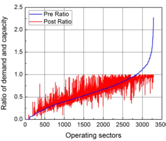
Fig. 6. Ratios of demand and capacity for pre- and post-regulation.
1,305 lateral and 1,379 vertical alternative trajectories are generated by airspace users and thereby fed back to the Network Manager. The missing ones are due to the fact that some hotspot airspaces may be located near the airports which, however, can not be avoided either in lateral or vertical. Generally, there are in total 8,939 (6,255 initial + 1,305 lateral + 1,379 vertical) trajectories scheduled for 6,255 flights. The problem dimensions are summarized in Table II.
B. Overall demand and capacity balancing
The ratios of demand and capacity are sorted (based on pre-regulation) and presented in Fig. 6. Obviously, the curves representing pre-regulation are steeper with some parts grow-ing higher than 1, meangrow-ing that for those operatgrow-ing sectors (i.e., elementary/collapsed sectors activated as a whole during particular time periods) the flight entries are higher than their capacities. After the regulation, however, it can be seen that all the exceeding demands have been balanced below the respective operating sectors’ capacities, and the curves turn to be level and average with respect to the post-regulation cases, which means more airspace capacities are well utilized.
Worth noting that in realistic operations a certain amount of capacity overloads are usually allowed (and in some cases the allowance can be quite large). This could be due to several reasons, such as the lack of initial schedules for pop-up flights, the conservative method for capacity evaluation, and the current way of counting traffic demand (i.e., flight entry rate) without considering the factors of occupancy, traffic pattern and complexity. Nevertheless, for the illustrative purpose, no capacity allowance is allowed in this study.
C. Trajectory options and delay management
As discussed in Sec. II-C, it is clear that any of the measures can be combined together and imposed on a particular flight. For example, to achieve the global optimum, a flight might be asked to fly its lateral alternative trajectory, experience some ground holding at the origin airport, undertake a small amount of airborne or linear holding en route, whilst being allowed to partially recover those delays along the remaining trajectory.
TABLE IV
BENCHMARK OF ASSIGNED DELAYS AND AFFECTED FLIGHTS.
Cases Total delayed flights (a/c) Total delay (min)
CASA 2,510 406,042
CDCB GH mode 1,840 219,862
Table IV presents a set of benchmark results, namely, implementing CASA (Computer Assisted Slot Allocation) and CDCB (with GH mode) to solve exactly the same problem. CASA is a function within Eurocontrol’s ETFMS (Enhanced Tactical Flow Management System) that follows the principle of RBS and matches traffic demand and airspace capacity by delaying flights’ departure times [18]. On the other hand, CDCB (with GH mode) means that all the measures mentioned above will be disabled, except for ground holding, so that it seems quite similar to CASA. The key difference, however, is that the RBS “constraint” is not respected for CDCB (GH mode). As Table IV shows, only about half of the delays are required by CDCB (GH mode) with respect to those needed by CASA (note that the reason of issuing such a huge amount of delay has been discussed in Sec. IV-B). This reveals, on some level, the trade-off between efficiency (i.e., minimizing the total delay cost in CDCB-GH mode) and fairness (i.e., obeying the RBS principle in CASA).
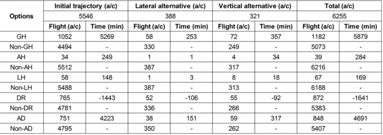
For the full-version CDCB, the detailed results of trajectory options and delay management can be seen in Table III. The most promising result would be that the total (arrival) delay is reduced to 4,691 min (see Table III). Remember when using CDCB in GH mode, it is greater than 200,000 min (see Table IV), which means that the delay reduction (by using the full CDCB) is nearly 98%. Nevertheless, it must be noted that, in compensation with the remarkable reduced delays, there are 709 (388 lateral + 321 vertical) flights diverted to their alternative trajectories. Furthermore, when comparing the total number of regulated flights, the difference between CDCB-GH mode and CDCB-full mode is relatively small. For the GH mode, the only available measure is ground holding, and there are 1,840 flights captured (see Table IV). For the full version, on the other hand, the regulated flights (i.e., performing any of the available measures) are at least 1,768.
Among the different ways, ground holding is obviously the most used, absorbing almost all the required system delays, but it appears in Table III that a small amount of airborne holding (284 min) and linear holding (169 min) could contribute to minimizing the total cost even if their unit cost is higher (than the cost of ground holding). This is due to the fact that if any delay must be transferred from the capacity-affected area to the origin airport by means of ground holding, then it is always the largest delay that will be issued once different delays are actually required for different sectors (within the network) that the flight traverses. In addition, delay recovery has the same effects as well because some available capacity (or empty slot), caused from delaying a flight, can be taken by the other flight that is able to advance its arrival time to the certain place, which is similar to an intermediate slot swapping process.
TABLE III
SUMMARY OF TRAJECTORY OPTIONS AND DELAY MANAGEMENT FORCDCB-FULL VERSION.
V. CONCLUSIONS AND FURTHER WORK
This paper presented a preliminary framework for collab-orative demand and capacity balancing. Airspace users could precisely schedule the alternative trajectories for their flights, based on the hotspot-oriented avoidance information generated and shared by the network manager. The alternative trajectory options are thereby submitted and subject to a global optimiza-tion, determining the best trajectory selection for each flight and the optimal distribution of possible delay assignments. While the alternative trajectory proved to effectively reduce delays, there still exist some open questions in future work:
(1) Airspace users must well participate in the collaborative trajectory submission process, and model accurately their cost structure (such as how much delay and fuel cost), as the network manager will optimize the overall cost for all the flights according to their provided information. Otherwise, the assigned solution to their flights might be unsuitable and could incur unnecessary environmental impact (e.g., extra fuel consumption) as well as vicious competition issues.
(2) When airspace users generating alternative trajectories, only the hotspots that are identified based on the initial trajec-tories can be bypassed (through lateral re-routing or vertical avoidance), without taking into account the impact of the newly submitted alternative trajectories. A possible solution for future research would be to further include the dynamic sectorization in the optimization model to synchronize the time management of traffic demand and airspace capacity.
(3) Uncertainty factors (e.g., in trajectory and capacity) have not been considered. Although the study is aimed at the pre-tactical phase, for the purpose of developing a robust model it is still worth exploring. Along with the requirement of question (1), a higher computational performance is needed in regard of the linear programming part. Using decomposition methods and/or meta-heuristic algorithms could be a solution, and will be subject to our future research.
REFERENCES
[1] M. Ball, C. Barnhart, G. Nemhauser, and A. Odoni, “Air transportation: Irregular operations and control,” Handbooks in Operations Research
and Management Science, vol. 14, pp. 1–67, 2007.
[2] FAA,Traffic Flow Management in the National Airspace System,
FAA-2009-AJN-251, 2009.
[3] N. V. Pourtaklo and M. Ball, “Equitable allocation of enroute airspace resources,” inProceedings of the 8th USA/Europe Air Traffic
Manage-ment Research and DevelopManage-ment Seminar, Napa, CA, 2009, p. 6.
[4] EUROCONTROL, “ATFCM operations manual - network operations handbook,” EUROCONTROL, Tech. Rep. Ed. 21.0, 2017.
[5] M. O. Ball, R. Hoffman, D. Lovell, and A. Mukherjee, “Response mechanisms for dynamic air traffic flow management,” inProceedings
of the 6th Europe-USA ATM Seminar. Baltimore. US, 2005.
[6] FAA, “Collaborative trajectory options program (ctop): Document infor-mation.” Federal Aviation Administration, Tech. Rep. AC 90-115, 2014. [7] M. E. Miller and W. D. Hall, “Collaborative trajectory option program demonstration,” in34th IEEE/AIAA Digital Avionics Systems Conference
(DASC), Prague, Czech Republic. IEEE, 2015, pp. 1C1–8.
[8] O. Rodionova, H. Arneson, B. Sridhar, and A. Evans, “Efficient trajec-tory options allocation for the collaborative trajectrajec-tory options program,”
in2017 IEEE/AIAA 36th Digital Avionics Systems Conference (DASC),
Sept 2017, pp. 1–10.
[9] P. E. Hart, N. J. Nilsson, and B. Raphael, “A formal basis for the heuristic determination of minimum cost paths,”IEEE transactions on Systems
Science and Cybernetics, vol. 4, no. 2, pp. 100–107, 1968.
[10] L. Delgado, “European route choice determinants,” 2015.
[11] R. Dalmau and X. Prats, “Fuel and time savings by flying continuous cruise climbs: Estimating the benefit pools for maximum range oper-ations,” Transportation Research Part D: Transport and Environment, vol. 35, pp. 62–71, 2015.
[12] R. Dalmau, M. Melgosa, S. Vilardaga, and X. Prats, “A fast and flexible aircraft trajectory predictor and optimiser for atm research applications,”
in 8th International Conference for Research in Air Transportation
(ICRAT), Castelldefels, Spain, 2018, paper submitted.
[13] Y. Xu, R. Dalmau, and X. Prats, “Maximizing airborne delay at no extra fuel cost by means of linear holding,”Transportation Research Part C:
Emerging Technologies, vol. 81, pp. 137–152, 2017.
[14] Y. Xu and X. Prats, “Effects of linear holding for reducing additional flight delays without extra fuel consumption,”Transportation Research
Part D: Transport and Environment, vol. 53, pp. 388–397, 2017.
[15] S. Zelinski and C. F. Lai, “Comparing methods for dynamic airspace configuration,” in Digital Avionics Systems Conference (DASC), 2011
IEEE/AIAA 30th. IEEE, 2011, pp. 3A1–1.
[16] D. Bertsimas and S. S. Patterson, “The air traffic flow management problem with enroute capacities,”Operations research, vol. 46, no. 3, pp. 406–422, 1998.
[17] Y. Xu and X. Prats, “Including linear holding in air traffic flow management for flexible delay handling,”Journal of Air Transportation, vol. 25, pp. 123–137, 2017.
[18] A. Cook, European air traffic management: principles, practice, and