Robust multivariate methods in Chemometrics
Peter Filzmoser
1Sven Serneels
2Ricardo Maronna
3Pierre J. Van Espen
41
Institut f¨ur Statistik und Wahrscheinlichkeitstheorie,
Technical University of Vienna, Vienna, Austria
2
Statistics and Chemometrics Group, Shell Global Solutions,
Shell Research and Technology Centre, Amsterdam, The Netherlands
3Department of Mathematics, National University of La Plata, Argentina
4
Department of Chemistry, University of Antwerp, Belgium
Abstract
This chapter presents an introduction to robust statistics with appli-cations of a chemometric nature. Following a description of the basic ideas and concepts behind robust statistics, including how robust esti-mators can be conceived, the chapter builds up to the construction (and use) of robust alternatives for some methods for multivariate analysis fre-quently used in chemometrics, such as principal component analysis and partial least squares. The chapter then provides an insight into how these robust methods can be used or extended to classification. To conclude, the issue of validation of the results is being addressed: it is shown how uncertainty statements associated with robust estimates, can be obtained. Keywords: robust statistics, robustness, location, scale, regression, M estimators, principal component analysis, partial least squares, linear dis-criminant analysis, D-PLS, validation, bootstrap, prediction interval.
Contents
1 Introduction 5
1.1 The concept of robustness . . . 5
1.2 Visualising multivariate data for outlier identification . . . 6
1.3 Masking effect . . . 6
1.4 Swamping effect . . . 7
1.5 Majority fit . . . 9
1.6 Is robustness a synonym to wasting information? . . . 10
2 Designing robust multivariate estimators 10 2.1 Which properties should a robust estimator have? . . . 10
2.1.1 Empirical influence function and influence function . . . . 10
2.1.2 Maxbias curve . . . 12 2.1.3 Breakdown point . . . 12 2.1.4 Statistical efficiency . . . 13 3 Robust regression 14 3.1 M-estimators . . . 15 3.2 Computing M-estimators . . . 16
3.3 Robust measures of residual size . . . 16
3.3.1 Scales based on ordered values . . . 17
3.3.2 Scale M-estimators . . . 17
3.3.3 Calibrating scales for consistency . . . 17
3.4 Regression estimators based on a robust residual scale . . . 18
3.4.1 The LMS and LTS estimators . . . 18
3.4.2 Regression S estimators . . . 18
3.5 The subsampling algorithm . . . 18
3.6 Regression MM-estimators . . . 19
3.7 Robust location and covariance . . . 19
3.7.1 Affine equivariance . . . 19
3.7.2 Asymptotic breakdown point . . . 20
3.7.3 The MCD estimator . . . 21
3.7.4 Multivariate S estimators . . . 23
3.7.5 Multivariate MM estimators . . . 23
3.7.6 The Stahel-Donoho estimator . . . 23
3.7.7 Using spatial signs . . . 24
3.8 Projection pursuit . . . 25
4 Robust alternatives to principal component analysis 27 5 Robust alternatives to partial least squares 29 5.1 A brief introduction to PLS . . . 29
5.2 Robustifying PLS . . . 30
5.2.1 Projection pursuit . . . 30
5.2.2 Robust covariance estimation . . . 31
5.2.3 Robust PLS by robust PCA . . . 33
5.2.4 Robust PLS as a partial version of robust regression . . . 33
5.3 Simulation results . . . 34
5.3.2 Bias and breakdown . . . 36
5.4 An application . . . 36
5.4.1 Application of robust techniques . . . 36
5.4.2 Prediction of the concentration of metal oxides in archæo-logical glass vessels . . . 37
5.4.3 Summary . . . 39
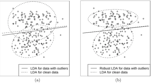
6 Robust approaches to discriminant analysis 39 6.1 Discriminant analysis . . . 39
6.2 Robust LDA . . . 41
6.3 Robust Fisher LDA . . . 43
6.4 Discriminant analysis ifp > n . . . 44
6.4.1 Singular value decomposition as a preprocessing step . . . 44
6.4.2 LDA in a PCA score space . . . 45
6.4.3 LDA in a PLS score space . . . 46
6.4.4 D-PLS . . . 46
7 Validation 47 7.1 Precision and uncertainty . . . 47
7.1.1 How to evaluate uncertainty for robust estimators? . . . . 47
7.1.2 The bootstrap . . . 47
7.1.3 The robust bootstrap . . . 49
7.1.4 Computational efficiency . . . 51
List of Abbreviations
CV cross-validation
D-PLS discrimination partial least squares EIF empirical influence function EPXMA electron probe x-ray micro-analysis
IF influence function
IRPLS iteratively re-weighted partial least squares IRWLS iteratively re-weighted least squares LAD least absolute deviation
LDA linear discriminant analysis LIBRA Library for Robust Analysis LMS least median of squares
LS least squares
LTS least trimmed squares MAD median absolute deviation MATLAB Matrix Laboratory
MCD minimum covariance determinant
MSE mean squared error
OLS ordinary least squares PARAFAC parallel factor analysis
PC principal component
PCA principal component analysis PCR principal component regression PLAD partial least absolute deviations
PLS (uni- or multivariate) partial least squares PLS2 multivariate partial least squares
PM partial M
PP projection pursuit
PP-PLS projection pursuit partial least squares
PRM partial robust M
QDA quadratic discriminant analysis
RAPCA reflection-based algorithm for principal component analysis RCR robust continuum regression
RMSE root mean squared error
RMSECV root mean squared error of cross validation RMSEP root mean squared error of prediction
ROBPCA robust PCA (one specific method by Hubertet al.32) RSIMPLS robust SIMPLS (one specific method by Hubertet al30) SPC spherical principal components
SVD singular value decomposition
TOMCAT Toolbox for Multivariate Calibration Techniques tri-PLS trilinear partial least squares
1
Introduction
1.1
The concept of robustness
Many statistical methods are based on distributional assumptions. Especially the normal distribution takes on a primordial role: well-known optimality prop-erties of the most frequently applied estimators do only hold at the normal model. For instance, the least squares estimator for regression is known to be the maximum likelihood estimator at the normal model. Nearly all regression methods which are common in chemometrics, are to some extent derived from least squares. This implies that the normal distribution assumes a key position in multivariate chemometric methods.
In practice data do never exactly follow the normal distribution. In most cases the normality assumption is satisfactory and methods based on it will produce reliable results. However, sometimes the normality approximation to the data is rather poor or even completely wrong. Data may intrinsically follow a different distribution than the normal (e.g. think of counting statistics such as X-ray counts which are Poisson distributed). The data may also show bi- or multimodality because the individual cases have been drawn from different pop-ulations. Here one can think of a data set containing cases which are known to appertain to different groups, but for which a joint calibration model is desired. E.g. different types of wines need to be analysed for their ester concentration. From the offset it is known that samples of different years and soils have differ-ent properties and thus belong to differdiffer-ent populations. Nevertheless a model which predicts the ester concentration reliably independently of their origin or year may be required. For such a model probably a regression technique will be used, albeit it is clear that the data were not generated by a single nor-mal distribution. Alternatively, the data may have been generated by the same model but have been influenced by different processes. Samples may have been generated in a similar manner but have undergone exposition to different effects (temperature, light, etc.), changing their behaviour, such that the assumption of a single distribution becomes invalid.
The normality assumption may also be violated by an entirely different pro-cess. Outliers may occur which have atypical properties compared to the major-ity of the data. Outliers can be generated in several ways: they can be objects which intrinsically have different properties or they can be artifacts produced by the data generation process. A typical example in chemometrics would be that some cases have been measured with a different light source or detector such that the spectra cannot be included in a single model with the regular cases. When outliers are present in the data it does not make sense to model the data distribution including the outliers. The true model according to which the non-outlying data points have been generated will differ significantly from a model estimated by data containing outliers.
All the above situations (multimodality, outliers) are examples of situations where the data do not follow a normal model. Whereas they are all examples of nonnormality, robust methods have explicitly been developed for the last men-tioned situation. Robust estimators are estimators derived for a given model, including slight deviations from this model. More precisely, if the main group of data points is assumed to come from a distributionG, then a robust estimator for such data is designed for the distribution Gε = (1−ε)G+εH, where H
0 2 4 6 8 0 2 4 6 8
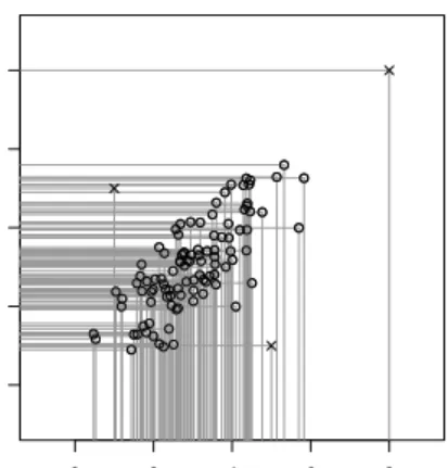
Figure 1: Bivariate normally distributed data cloud (◦) and three outliers at different positions (×) as well as the projection of each point onto both axes.
is another distribution and ε ∈ [0,1). Because robust estimators are usually especially designed for such ε contaminated distributions, they should resist any type of moderate deviation from G. This implies that robust estimators can in practice also perform well at distributions which are close to G. For instance, if Gis the normal distribution, then robust estimators are designed for a normal contaminated with outliers coming from a given outlier generating distributionH, but they may perform well as well for heavier tailed “close to normal” distributions such as the Cauchy and Student’st distributions.
1.2
Visualising multivariate data for outlier identification
Detection of either multimodality or outliers is straightforward for univariate and bivariate data. For multivariate data clouds it will be difficult or even impossible to visualise the data and graphically detect the outliers. In partic-ular chemometric calibration and classification problems are usually of a high dimensional nature: e.g. in spectrophotometry, the spectra are commonly mea-sured at p > 1000 variables. Visual inspection by simply plotting the data is practically impossible as one would need to inspect plots of all possible pairs of two variables. Even then the outliers can be of a multivariate nature such that they will not be detected by inspecting only two dimensions. Consider the reduction of a bivariate problem to one variable. In Figure 1 a bivariate distri-bution is plotted. Three outliers are added; it can be seen that a projection of the data onto either one of both axes does only reveal one of the three outliers. It is straightforward to imagine that a similar effect occurs when one projects multivariate data on two dimensions.
1.3
Masking effect
Instead of simply projecting the data onto a pair of its variables, classical sta-tistical methods can be used for data reduction. A straightforward approach is
0 2 4 6 8 10 12 2 4 6 8 10 12 −2 0 2 4 6 8 −4 −2 0 2 4 −2 0 2 4 6 Component 1 Component 2 (a) (b)
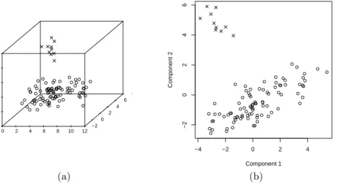
Figure 2: Trivariate normally distributed data cloud (◦) and a group of outliers (×); plotted are (a) the data and (b) a scatterplot of PC1 vs. PC2
summarise the data into principal components and then making pairwise plots of these principal components. Alternatively, if a dependent variable exists as well, a data reduction technique can be used which takes into account the relation to the predictand, such summarising the data into latent variables by partial least squares or canonical correlation analysis. However, methods like principal com-ponent analysis or partial least squares are classical (i.e. nonrobust) estimators, which implies that the outliers do also have an effect on the estimates of the latent variables obtained by those methods. The estimated latent variables can be biased in such a way that in fact no outliers are detected. The effect that due to the outliers’ presence one is not able to detect them is referred to as the
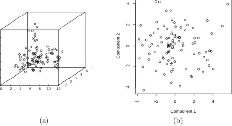
masking effect. In Figure 2 we show a trivariate data distribution to which a cluster (ten percent) of outliers has been added. In the left subplot the data are shown as a three dimensional plot; the right subplot shows a biplot of the first two principal components (PCs) of this data set. In Figure 3 similar plots are shown for the same data cloud where the outliers have been added at a different position. From Figures 2 and 3 we see that it depends on the position in space where the outliers are situated whether principal components reveal them or not. A good robust data reduction method (discussed more into detail later in this chapter) would reveal the outliers in both configurations, whereas it would also still yield reasonable results if the data are not contaminated by any type of outliers.
1.4
Swamping effect
Apart from the masking effect, outliers can also cause typical points to be iden-tified as outliers. This is easily understood by taking regression as an example. Figure 4 shows a typical regression problem with normally distributed data to which a group of outliers is added. The least squares regression tries to fit all data points, i.e. also the outliers, and is thus attracted towards the outliers. Normally one would assign outliers to a least squares fit as those points which
0 2 4 6 8 10 12 2 3 4 5 6 7 8 9 −2 0 2 4 6 8 −4 −2 0 2 4 −4 −2 0 2 4 Component 1 Component 2 (a) (b)
Figure 3: Trivariate normally distributed data cloud (◦) and a group of outliers (×); plotted are (a) the data and (b) a scatterplot of PC1 vs. PC2
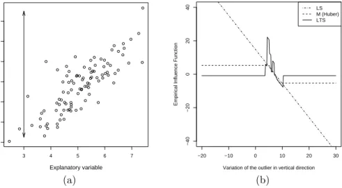
0 5 10 15 20 5 10 15 20 Explanatory variable Response variable
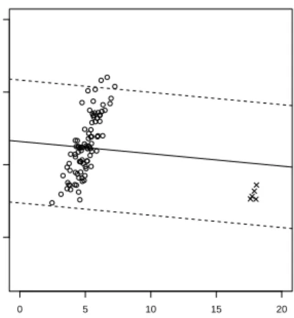
Figure 4: A typical regression problem with normally distributed errors; a cloud of outliers has been added. The solid line shows the least squares fit to the data. The dotted lines show the limits beyond which points are considered to be outlying.
0 5 10 15 20 5 10 15 20 Explanatory variable Response variable
Figure 5: The regression problem from Figure 4 after removal of the outliers detected there.
have the highest residuals to the model. In Figure 4 the regression line is shown together with two dashed lines indicating a residual distance of two standard errors. Potential outliers will fall outside these bands. In the example shown, the points having the largest residuals, which are thus detected “outliers” are in this case not the true outliers, but typical points which are far away from the regression line just because the latter badly fits the majority of the data. The effect that regular data points are identified as outliers is denominated the
swamping effect.
The above figures show two main effects of outliers. At first the outliers themselves are hard to detect (remember that in a multivariate setting, a plot which shows the entire data distribution cannot be constructed). Secondly, the outliers cause the regression line to be severely distorted. Predictions of future responses made according to this line will be unreliable. At this point one would intuitively proceed by detection of the outliers after which the regression analysis is performed on the remaining points. But exactly due to the masking and swamping effects the wrong data points may be identified as outliers such that eventually the regression analysis on the assumed “clean” data remains a jeopardy. In Figure 5 we show what happens if one would proceed by omitting the identified outliers in Figure 4. Some of the good data points have been removed; the true outliers are still present. The slope of the regression line is still erroneous due to the outliers and the latter are still not detected.
1.5
Majority fit
The goal of robust methods is to estimate parameters under conditions of slight deviations to the model. Once the parameters are estimated in a robust way it is possible to identify outliers which are considered to be deviating data points ac-cording to the underlying statistical model. It should be observed that outlier detection always involves some subjectivity, while parameter estimation does not. Gross outliers can be detected and henceforth omitted from the analysis.
Apart from these, various other deviations from the underlying model may be present such as a small groups of points which are known to have slightly dif-ferent properties but cannot be omitted. In this case it is not possible to delete the deviating data points prior to a classical analysis. Nonetheless the classi-cal analysis may probably accord too great an importance to the few differing points. A well chosen robust estimator will provide a reliable fit for the whole range spanned by the data points without being influenced by deviating points, regardless the type of deviation. Even gross outliers may be present in the data without influencing the robust fit.
Most robust methods may be described as classical methods where the data are weighted, with weights depending on the data. The majority of the data will receive a (quasi) uniform weight while the more atypical individual cases are, the lower the weight they will get. Summarising, a robust fit can be considered to be a majority fit, where the fraction of data which makes up the majority depends on the points in space of the individual cases.
1.6
Is robustness a synonym to wasting information?
Many early robust estimators were based on trimming (e.g. the well known least trimmed squares estimator for regression where a pre-determined percentage of the largest squared residuals is trimmed and thus not considered for finding the regression parameters). On the other hand, trimming is not done forany data points, but especially for the largest and smallest values. If any data points would be trimmed, the precision (or efficiency) of the resulting estimator would be much lower than that where the extremes are trimmed. This fact underlines already that even trimming does not “waste” information. Ideally, robust esti-mation techniques should only discard data points which are extremely distinct from the bulk of data and are thus very likely to be gross outliers. All other data points should to some extent be taken into account. The amount of infor-mation taken from each data point is then regulated by weights between 0 and 1 given to them. This procedure will in general lead to estimators with higher efficiency.
2
Designing robust multivariate estimators
2.1
Which properties should a robust estimator have?
Robust estimators should be resistant to a sizeable proportion of outliers or deviation from assumptions. They should also still yield reasonable results if these ideal assumptions are valid. In this section some tools are introduced to assess an estimator’s robustness properties: the influence function, the maxbias curve and the statistical efficiency.
2.1.1 Empirical influence function and influence function
One of the basic ideas of robustness is that a robust estimator should not be influenced by a limited amount of contamination, regardless where this contam-ination is situated. A simple way to check the behaviour of an estimator under small contamination is to vary a single data point. As an example, Figure 6 shows the effect of an observation which is varied in space to different regression
3 4 5 6 7 6 8 10 12 14 16 18 Explanatory variable Response variable −20 −10 0 10 20 30 −40 −20 0 20 40
Variation of the outlier in vertical direction
Empirical Influence Function
LS M (Huber) LTS
(a) (b)
Figure 6: Empirical influence functions for regression estimators. Subplots show (a) the data with varying positions of the outlier and (b) the empirical influence functions of the slope parameter estimated by least squares (LS), M regression and least trimmed squares (LTS).
estimators. The data were taken from a normal distribution. The position of one data point was changed as is shown in Figure 6a. For each position of the data point, we are interested in the change of the slope parameter of the fol-lowing regression estimators: least squares regression and two robust regression estimators: Huber M regression27 and LTS regression estimators (see later in
this chapter). The result is known as the empirical influence function (EIF), but in order to make the results of the different estimators comparable, we compute the difference of the slopes for the contaminated and uncontaminated data, and divide by the amount 1/nof contamination. The right subplot of Figure 6 shows the results. It can be seen that the least squares estimator has an unbounded EIF. This means that a single gross outlier can have an arbitrarily large effect on the estimator. Both robust estimators possess a bounded EIF. However, not only the bound but also the shape of the EIF is of importance in order to under-stand how a robust estimator deals with contamination. Ideally the EIF should be smooth: it should not show local spikes or should not be a step function. In practice, the effect of placing a data point at one location and then shifting it to a very close position should be very small. One observes that indeed the M estimator has a smooth EIF and is thus virtually insensitive to local shifts in the data. On the contrary, the response of the least trimmed squares estimator to small data perturbations is far from smooth (in the literature it is said to be prone to a highlocal shift sensitivity).
The concept of the EIF can be formalised by the so-called influence function (IF). The IF measures the influence an infinitesimal amount of contamination has on an estimator with respect to its position in space.24 More precisely, the
influence function of an estimatorT at a given distributionGis defined as:
IF(z, T, G) = lim
ε↓0
T[(1−ε)G+εδz]−T(G)
where εis the fraction of contamination andδz is a probability measure which puts all the mass at z. The point z can be any point in the p dimensional space but in practice it will often be a measured data point. Evaluating the influence function at the points of a data set reveals how each data point changes the estimator’s behaviour. The influence of an outlier in the data set on the estimator can be measured by evaluating the influence function at the outlier. For nonrobust estimators evaluation of the influence function at the outlier will yield significantly different results compared to evaluating the IF at the typical data, whereas for a robust estimator the effect will be limited.
2.1.2 Maxbias curve
Hitherto we have considered the influence of a limited amount of contamina-tion at varying posicontamina-tions in space. An interesting quescontamina-tion is what happens if instead of the position in space one changes the proportion of contamination. What one expects is that a robust estimator can withstand a certain fraction of contamination. The mathematical tool to examine to which extent an esti-mator is distorted with respect to the fraction of contamination in the data is the maxbias curve. The maxbias curve measures the bias an estimator has with respect to the percentage of the worst possible type of contamination. LetZbe the original data set and ˇZ be a data set in whichmout ofnobservations have been replaced with arbitrary values and let k · kdenote the Euclidean norm, then the maxbias curve for an estimator T is defined as:
maxbias(m, T, Z) = sup ˇ
Z
kT( ˇZ)−T(Z)k. (2)
It is known that for some estimates of regression the worst possible type of outliers is found at points where y,xand the fraction y/xincrease to infinity. In what follows a numerical example is shown which does not reflect the exact maxbias curve but illustrates what happens if bad (but not the worst type) of outliers are added to data for the regression problem discussed in the previous section. For the data set presented in Figure 6, we have added vertical outliers in the following manner: points were added in a range (µx+a, µy+b) about
the mean, wherea ∈[0,10] and b ∈[104,105]. We then computed the bias of the slope compared to the known regression slope. In Figure 7 we see that the bias of the least squares estimator tends to infinity if a single observation is replaced by bad outliers. The other robust estimators exhibit a moderate bias up till a certain point where they also break down. To conclude we note that if the outliers’ position in xwould have been put further away from the data cloud too (leverage points), then we would observe a faster breakdown for the robust M regression method displayed here, as this method is known to be only resistant to outliers in y.
2.1.3 Breakdown point
From the bias curves one observes that for each estimator, there exists a point where the bias tends to infinity withε. This point is referred to as thebreakdown point. Loosely, the breakdown point indicates which percentage of the data may be replaced with outliers before the estimator yields aberrant results. Based on
0 10 20 30 40 50 60 70 0.0 0.5 1.0 1.5 2.0 Fraction of contamination in % Maximum bias LS M (Huber) LTS
Figure 7: The regression problem from Figure 4 after removal of the outliers detected there.
the maxbias curve, for finite samples the breakdown point is given by:
ε∗ n(T, Z) = min nm n; maxbias(m, T, Z) =∞ o . (3)
Forn→ ∞ one obtains theasymptotic breakdown point, denotedε∗. For least
squares regression it holds that ε∗ = 0. The maximal possible value of the
asymptotic breakdown point equals 1. However, estimators satisfying equiv-ariance conditions1 have a maximal asymptotic breakdown point of 0.5, which means that the typical points must out-number the outliers in order to produce meaningful results. One of the goals in designing robust estimators is obtain-ing a high breakdown point. Howbeit, bounded influence and high breakdown should not result in a drastic decrease in efficiency.
2.1.4 Statistical efficiency
An important property to any statistical estimator is the variance. It is well known that many parametric estimators have optimality properties at their un-derlying model. For instance, the maximum likelihood estimator for the linear regression model with normally distributed error terms is the least squares es-timator. The least squares estimator is also the minimum variance unbiased estimator for the linear model (the Gauß-Markov theorem). This implies that predictions made by any other regression estimator for data which follow the lin-ear model with normally distributed error terms, will have a higher uncertainty 1Equivariance conditions are deemed reasonable for most estimating problems, e.g. loca-tion, covariance and regression; for the definition of affine equivariance see Section 3.7.1 and for the definition of scale equivariance see Section 3.3.
than the least squares predictions. So also robust estimators for regression are prone to an increase in variance compared to least squares. This statement may be generalised to other settings than regression; it can be stated that robust estimators always have a higher variance than classical parametric estimators if evaluated at the underlying model of the parametric estimator. They are said to be less efficientthan parametric estimators. So as to design robust es-timators it is important not only to investigate the robustness properties but also the efficiency properties. One could even conjecture that for chemometric robust estimators, efficiency is a more important property than robustness in the breakdown sense. Data sets for multivariate calibration hardly ever contain 50% of outliers. Moreover, a few outliers very far away from the data cloud would readily be detected by inspecting the data. What is occurring more fre-quently is a data set which slightly deviates from normality (the most frefre-quently assumed underlying distribution) without any gross outliers being present. For such data a robust estimator will outperform the classical estimator because the latter is only optimal at the exact normal model, given it is efficient, such that the effect of increase in variance of the robust estimator does not compensate for the classical estimator’s loss in precision due to deviation from normality.
3
Robust regression
Regression assumes a key position in chemometrics. Apart from being applied as a method in its own right, it is also a part of more complex estimators such as partial least squares or three-way methods. One way to develop robust alternatives to these methods is by replacing the classical regressions by robust ones. In that case the properties of the entire method derive from the type of robust regression used. In this section we present an overview of some of the most useful robust estimators for regression.
The data of a regression situation are then×pmatrixXof predictor variables with elements xij and the n−vector y with elements yi. For regression with
intercept we assume that the first column of the data matrix is a column of ones. Callxi= (xi1, . . . , xip)T the column vector containing the elements of the
i-th row ofX. The linear regression model is then given by
yi=xTi β+ei, i= 1, ..., n, (4)
where the unknown regression parameter β is a p-vector and ei denotes the
error terms, which are assumed to be i.i.d. random variables. For a given estimator ˆβcallri=ri
³
ˆ
β´=yi−xTi βˆ thei-th residual. Most
regression estimators are based on a minimisation of the size of the residuals. The classical least squares (LS) estimator is defined as
ˆ βLS= arg min β n X i=1 ri(β)2. (5)
An ancient alternative to LS is theL1 estimator defined as ˆ β= arg min β n X i=1 |ri(β)|. (6)
3.1
M-estimators
The LS estimator is not robust, in the sense that atypical observations may uncontrollably affect the outcome. The reason is that a large residual would dominate the sum (5). One way out of this difficulty is to define a more general family of estimators. Note that (5) and (6) can be written as:
ˆ β= arg min β n X i=1 ρ(ri(β)), (7)
where ρ(r) = r2 for LS and ρ(r) = |r| for L
1. By taking other ρ functions different estimators are obtained. In fact, equation (7) is the definition of a whole class of estimators commonly referred to asM-estimators.
Note that if ˆβ is the LS estimate, then transforming y to ty with t ∈ R
transforms ˆβtotβ. This property, calledˆ regression equivariance, is not shared by the estimator (7), except when ρ(z) =|z|a for some a. To make estimator
(7) scale equivariant, we define in general a regression M-estimator by
ˆ β= arg min β n X i=1 ρ µ ri(β) ˆ σ ¶ , (8)
where ˆσis a robust scale estimator of the residuals, that can be estimated either previously or simultaneously with the regression parameters.
The functionρmust be chosen adequately. Recall that we want an estimate to be (a) robust in the sense of being insensitive to outliers, and (b) efficient in the sense of being similar to LS when there are no outliers. For (a) to hold,
ρ(r) must increase more slowly than r2 for larger, and for (b),ρ(r) must be approximately quadratic for smallr.
Differentiating (8) with respect to β we get that the estimate fulfils the system ofM-estimating equations
n X i=1 ψ µ ri(β) ˆ σ ¶ xi= 0 (9)
where ψ=ρ0.For LS,ψ(r) =r, and (9) are the well-known normal equations.
We may then in general interpret (9) as a robustified version of the normal equations, where the residuals are curbed. ForL1 we haveψ(r) = sign (r).In general, solutions of (9) arelocal minima of (8), which may or may not coincide with the global minimum.
PutW(r) =ψ(r)/r.Then (9) may be rewritten as
n X i=1 wi ¡ yi−xTiβ ¢ xi= 0 (10)
with wi =W(ri(β)/σˆ).Then (10) is a weighted version of the normal
equa-tions, and hence the estimator can be seen as weighted LS, with the weights depending on the data . For LS,W is constant. For an estimator to be robust, observations with large residuals should receive a small weight, which implies that W(r) has to decrease to zero fast enough for large r.
Ifψ is an increasing function, the estimate is calledmonotonic. A family of monotonic estimators which contains LS andL1as extreme cases is theHuber family, withρ0 given by
ψH,k(r) = ½
r for |r| ≤k
k sign (r) otherwise (11)
The extreme casesk→ ∞andk→0 correspond to LS andL1,respectively. Monotonic estimates have the computational advantage that (9) gives the
global minima of (8). But they may lack robustness ifXcontains atypical rows (the so-calledleverage points). The intuitive reason is that if somexiis “large”,
then thei-th term will dominate the sum in (10), which would be unfortunate if (xi, yi) is atypical (a “bad leverage point”). For this reason it is better to use
M-estimators given by (8) with abounded ρ.An example is thebisquarefamily, with ρB,k(r) = ( ¡r k ¢2³ 3−3¡r k ¢2 +¡r k ¢4´ for |r| ≤k 1 else . (12)
Bounded ρs present computational difficulties which will be discussed in the next Sections.
Whenk→ ∞ in (11) or (12), the corresponding estimate tends to LS and hence becomes more efficient and at the same time less robust. Thus k is a tuning parameter the choice of which is a compromise between efficiency and robustness. The usual practice is to choosek to attain a given efficiency, such as 0.90.
3.2
Computing M-estimators
Equation (10) suggests an iterative procedure to obtain local minima. As-sume we have an initial value ˆβ0. Call ˆβm the approximation at iteration m.
Then given ˆβm, compute the residuals ri = ri ³
ˆ βm
´
and then the weights
wi =W(ri/σˆ), and solve (10) to obtain ˆβm+1. The procedure is called
iter-ative reweighted least squares (IRWLS), and converges ifW(z) is a decreasing function of|z|(Maronna et al., 2006).41
Ifψis monotonic, the choice of ˆβ0 influences the number of iterations, but not the final outcome. But if ρ is bounded, then ψ tends to zero at infinity, which implies that there may be many local minima, and therefore the choice of ˆβ0 is crucial. Using a non-robust initial estimator like LS may yield “bad” local minima.
A good initial estimator is also necessary to obtain the scale ˆσ. If there are no leverage points one could use L1 as an initial ˆβ0, and compute ˆσ as a robust scale of the residualsri(ˆσ) (e.g. the MAD). But otherwise we need other
choices. The initial estimator should not need a previous residual scale. Before initial estimators can be considered, we present some further concepts.
3.3
Robust measures of residual size
Given r= (r1, ..., rn) we shall define a scaleσ(r) such that σ(tr) =|t|σ(r) for
3.3.1 Scales based on ordered values
Call |r|(i) the ordered absolute values of the ris: |r|(1) ≤ ... ≤ |r|(n). The simplest scale is aquantile ofr:
σ(r) =|r|(h) (13)
for some h∈ {1, .., n}. Forh=n/2 we have the median. Other choices will be considered below.
A smoother alternative is to consider a scale more similar to the standard deviation, namely thetrimmed squares scale
σ(r) = Ã 1 n h X i=1 |r|2(i) !1/2 , (14)
which forh=ngives the familiar root mean squared error (RMSE).
3.3.2 Scale M-estimators
Henceforth aρ-function will denote a functionρsuch thatρ(x) is a nondecreas-ing function of |x|, ρ(0) = 0, and ρ(x) is (strictly) increasing for x > 0 such that ρ(x)< ρ(∞).ifρis bounded, it is also assumed that ρ(∞) = 1.
An M-estimator of scale (anM-scale for short) is defined as the solutionσ
of an equation of the form 1 n n X i=1 ρ³ri σ ´ =δ (15)
whereρis aρ-function andδ∈(0, ρ(∞)).The choiceρ(z) =z2andδ= 1 yields the RMSE. The choiceρ(z) = I (|z|>1) andδ= 0.5 yieldsσ= med (|r|),where “med” denotes the median. We shall be interested in estimates withbounded ρ.
Equation (15) is nonlinear, but it is easy to solve iteratively. Put
Wσ(z) =ρ(z)
z2 . (16)
Then (15) can be rewritten as
σ2= 1 nδ n X i=1 wir2i
withwi =Wσ(ri/σ),which displays ˆσas a weighted RMSE. Given some
start-ing valueσ0,an iterative procedure can be implemented as was done for regres-sion M-estimators.
3.3.3 Calibrating scales for consistency
If z ∼ N¡0, σ2¢, then the standard deviation of z is σ by definition. The median of |z| is instead 0.675σ.Hence if we have a sample z1, ..., zn, then ˆσ=
med (|z1|, ...,|zn|) will tend to 0.675σfor largen, and therefore ˆσ/0.675 would
be an approximately unbiased estimate of σfor normal data.
In general, given a scale estimate ˆσ it is convenient to “normalise” it by dividing it through a constant c so that ˆσ/cestimates the standard deviation at the normal model. The M-scale (15) withρ=ρB,1 hasc=1.65.
3.4
Regression estimators based on a robust residual scale
Given β, letr(β) = (r1(β), ..., rn(β)). We shall consider an estimator of the
form
ˆ
β = arg min
β σˆ(r(β)) (17)
where ˆσis a robust scale.
3.4.1 The LMS and LTS estimators
If ˆσ is given by (13), we have the least quantile estimator. The case h=n/2 is the least median of squares (LMS) estimate. Actually, to attain maximum breakdown point one must take
h= · n+p+ 1 2 ¸ (18)
where [t] is the integer part oft. Estimators of this class are very robust in the sense of having a low bias, but their asymptotic efficiency is zero.
If ˆσ is given by (14), we have the least trimmed squares (LTS) estimator. Again, the optimalhis given by (18). Their asymptotic efficiency is about 7%.
3.4.2 Regression S estimators
Regression estimators with ˆσ given by (15) are called S-estimators. It can be shown that they satisfy the M-estimating equations (9) with ψ = ρ0; and it
follows that, given an initial approximation, they can be computed by means of the IRWLS algorithm. The boundedness ofρis necessary for the robustness of the estimate. But ifρis bounded, thenψis not monotonic, which implies that the equations yield onlylocal minima of ˆσ(r(β)),and hence a reliable starting approximation is needed. An approach to obtain an initial estimator is given in the next Section.
The efficiency of the S-estimator withρthe bisquare function is about 29%. In general, it can be shown that the efficiency of S-estimators cannot exceed 33%. Although better than LMS and LTS, S-estimators do not allow the user to choose a desired high efficiency. This goal is attained by the estimates to be described in Section 3.6.
3.5
The subsampling algorithm
The approach to find an approximate solution to (17) is to compute a ”large” finite set of candidate solutions, and replace the minimisation over β ∈Rp by
minimisingσb(r(β)) over that finite set. To compute the candidate solutions we take subsamples of sizep
{(xi, yi) :i∈J}, J ⊂ {1, ..., n}, # (J) =p.
For each J find βJ that satisfies the exact fit xT
i βJ = yi for i ∈ J. Then
the problem of minimising bσ(r(β)) forβ∈Rp is replaced by the finite problem
prohibitive unless both n and p are rather small, we choose N of them at random: {Jk:k= 1, .., N} and the initial estimateβbJk∗ is defined by
k∗= arg min©σb¡r¡β
Jk ¢¢
:k= 1, ..., Nª. (19) Suppose the sample contains a proportionε of outliers. The probability of an outlier-free subsample is α = (1−ε)p, and the probability of at least one
outlier-free subsample is 1−(1−α)N. If we want this probability to be larger
than 1−γ,we must have
lnγ≥Nln (1−α)≈ −N α and hence N ≥ |lnγ| |ln (1−(1−ε)p)| ≈ |lnγ| (1−ε)p (20)
forpnot too small. ThereforeN must grow exponentially withpif robustness is to be ensured.
3.6
Regression MM-estimators
We are now ready to define a family of estimators attaining both robustness and controllable efficiency. We shall deal with (8) where ρ(z) is abounded ρ -function. We assume that there is a previous estimator ˆβ0 which is robust but possibly inefficient (e.g. an S-estimator). Compute ˆβ0 and the corresponding residuals ri. Compute ˆσ as an M-scale (15) with ρ=ρB,1. Let ˜σ= ˆσ/c0 with c0 = 1.65. Now letρ = ρB,k with k chosen to have a given efficiency γ. We
recommendγ= 0.85 which impliesk= 3.44. Then compute ˆβas a local solution of (8) using the IRWLS starting from ˆβ0. The resulting estimator has the BP of ˆβ0and the asymptotic efficiencyγ.
It is shown by Maronna et al. (2006)41that if ˆβ
0is the bisquare S-estimator, then the resulting MM-estimator with efficiency 0.85 has a contamination bias not much larger than that of ˆβ0.
3.7
Robust location and covariance
Multivariate location and covariance play a central role in multivariate statis-tics because many multivariate methods directly build on these estimates. For example, principal component analysis is carried out on the centred data, and the standard method uses a decomposition of the covariance matrix to find the principal components. Outliers or deviations from a model distribution can lead to very different results, and thus it is necessary to robustly estimate mul-tivariate location and covariance. Many methods have been proposed for this purpose. Before discussing various approaches, we will first think about desired properties of robust location and covariance estimators. Aside from robustness issues, a central property is affine equivariance which will be discussed below.
3.7.1 Affine equivariance
It is desirable that location and covariance estimates respond in a mathemati-cally convenient form to certain transformations of the data. For example, if a
constant is added to each data point, the location estimate of the modified data should be equal to the location estimate of the original data plus this constant, but the covariance estimate should remain unchanged. Similarly, if each data point is multiplied by a constant, the new location estimate should be equal to the old one multiplied by the same constant, and the new variances should be the constant squared times the old variances. More general, one can define a transformation that is using a nonsingular p×pmatrix A and a vector b of length p to transform the p-dimensional observations x1, . . . ,xn by Axj+b.
This transformation performs any desired nonsingular linear transformation of the original data. Thus, if tdenotes a location estimator, it is requested that
t(Ax1+b, . . . ,Axn+b) =A·t(x1, . . . ,xn) +b, (21)
and for a covariance estimatorC we require
C(Ax1+b, . . . ,Axn+b) =A·C(x1, . . . ,xn)·AT. (22)
Location and covariance estimators that fulfil (21) and (22) are called affine equivariant estimators. These estimators transform properly under changes of the origin, the scale, or under rotations.
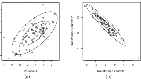
Figure 8a shows a bivariate data set where the location (+) was estimated by the arithmetic mean and the covariance by the sample covariance matrix. The latter is visualised by so-calledtolerance ellipses: In case of normally distributed data the tolerance ellipses would contain a certain percentage of data points around the centre and according to the covariance structure. Here we show the 50% and 90% tolerance ellipses. Figure 8b pictures the data after applying the transformation Axj+b= µ −2 3 1 −1 ¶ xj+b
to each data point. The location and covariance estimates were not recomputed for the transformed data but were transformed according to the equations (21) and (22). It is obvious from the figure that the transformed estimates are the same as if they would have been derived directly from the transformed data. Note that the transformation matrixAis close to singularity because the spread of the data becomes very small in one direction. The property of affine equivariance is only valid for nonsingular transformation matrices.
Affine equivariance is not only important for estimation of location and co-variance but also for multivariate methods like discriminant analysis or canonical correlation analysis. The results of these methods will remain unchanged under linear transformations. This is different for principal component analysis which is orthogonal equivariant but not affine equivariant. The results will only be properly transformed under orthogonal transformation matrices A.
3.7.2 Asymptotic breakdown point
The breakdown point (for simplicity, we will omit “asymptotic in this section) was already discussed in section 2.1.3 in the context of regression, and it is also used as an important characterisation of robustness for location and covariance estimators. Clearly, the breakdown points of the classical estimators, the arith-metic mean and the sample covariance matrix, are both 0 because even a single
1 2 3 4 5 6 7 4 6 8 10 12 Variable 1 Variable 2 −8 −6 −4 −2 0 2 0 5 10 Transformed variable 1 Transformed variable 2 (a) (b)
Figure 8: Bivariate data with estimated location (+) and covariance matrix (visualised by tolerance ellipses); plotted are (a) the original data and (b) the transformed data, together with the transformed estimates.
observation placed at an arbitrary position in space can completely spoil these estimators.
The simplest choice for a very robust location estimator would be the me-dian, computed for each variable. Since the median for univariate data has a breakdown point of 0.5, the coordinate-wise median would also have this break-down point. However, this estimator is not affine equivariant. For the data used in Figure 8a the median for the variables is (4.97,8.14) and for the transformed data in Figure 8b it is (−4.12,7.98). The transformation of the coordinate-wise median of the original data results in (−3.79,7.76). This difference would in general become larger if less data points were available.
The univariate median is that point which minimises the sum of the distances to all data points. A natural extension of this concept to higher dimensions is calledspatial medianorL1-median. It is defined as that point in the multivariate
space which minimises the sum of the Euclidean distances to all data points. The spatial median has good statistical properties: it has a breakdown point of 0.5. However, this multivariate location estimator is only orthogonal equivariant but not affine equivariant. Note that in the context of principal component analysis or partial least squares this would be sufficient because these methods are only orthogonal equivariant.
3.7.3 The MCD estimator
An estimator of multivariate location and covariance which is affine equivariant
and has high breakdown point is theMinimum Covariance Determinant(MCD)
estimator. The idea behind this estimator is in fact related to the LTS estimator from Section 3.4.1. Here, one is searching for those h data points for which the determinant of the (classical) covariance matrix is minimal. The location estimatortis the mean of thesehobservations, and the covariance estimatorC
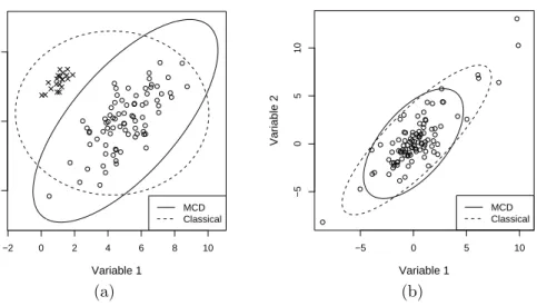
−2 0 2 4 6 8 10 0 5 10 Variable 1 Variable 2 MCD Classical −5 0 5 10 −5 0 5 10 Variable 1 Variable 2 MCD Classical (a) (b)
Figure 9: Tolerance ellipses (97.5%) based on the MCD estimator and on the classical sample mean and sample covariance matrix for (a) bivariate normally distributed data with outliers and (b) bivariateT2 distributed data.
by a constant to obtain consistency for normal distribution. The parameterh determines the robustness but also the efficiency of the resulting estimator. The highest possible breakdown point can be achieved if h≈n/2 is taken, but this choice leads to a low efficiency. On the other hand, for higher values of hthe efficiency increases but the breakdown point decreases. Therefore, a compromise between efficiency and robustness is considered in practice.
The computation of the MCD estimator is not trivial. While for a low num-ber of samples in low dimension in principle all subsets of hdata points can be considered in order to find the subset with smallest determinant of its covariance matrix, this is no longer possible for large n or in higher dimension. For this situation, a fast algorithm has been proposed which finds an approximation of the solution.47
It is important to note that the MCD estimator can only be applied to data sets where the number of observations is larger than the number of variables, which is a serious limitation for many applications in chemometrics. The reason is that ifp > nthen alsop > h, and the covariance matrix of anyhdata points will always be singular, leading to a determinant of 0. Thus, each subset of h data points would lead to the smallest possible determinant, resulting in a non-unique solution. In fact, a non-trivial solution can only be obtained ifhis smaller than the rank of the data.
Figure 9 shows a comparison between the MCD estimator and classical lo-cation and covariance estimation for two simulated data sets. The covariance estimates are visualised by 97.5% tolerance ellipses, the location estimates are the centres of the ellipses. In Figure 9a a bivariate normally distributed data set is used, where 20% of the data points are generated with a different mean and covariance. Note that these deviating data points cannot be identified as outliers by inspecting the projections on the coordinates. Not only the location estimate is influenced by the deviating points, but especially the covariance
structure. The data coming from the outlier distribution are inflating the tol-erance ellipse based on the classical estimators while that based on the MCD is much more compact and reflects the structure of the majority of data.
The second example shown in Figure 9b is simulated from a bivariate T
distribution with 2 degrees of freedom with a certain covariance structure. Also here the inflation of the classical ellipse due to some very distant points is visible. We can also compute the correlation coefficient using the classical and robust covariance estimates. In the first example the classical correlation is 0.00 while the MCD gives a correlation of 0.70, which is also the result of the classical correlation for the data without outliers. For the second example we obtain a value of 0.84 for the classical correlation and 0.60 for the robust correlation.
3.7.4 Multivariate S estimators
Similar as in the regression context (see Section 3.4.2), it is possible to define S estimators in the context of robust location and covariance estimation.9, 38 The idea is to make the Mahalanobis distances small. The Mahalanobis or multivariate distances are defined as
d(xi,t,C) = (xi−t)TC−1(xi−t) fori= 1, . . . , n
for a location estimatortand a covariance estimatorC. Note thatdis actually a squared distance. Thus, in contrast to the squared Euclidean distance
d(xi,t) = (xi−t)T(xi−t) fori= 1, . . . , n
the Mahalanobis distance also accounts for the covariance structure of the data. Small Mahalanobis distances can be achieved by using a scale estimator σand minimising σ(d(x1,t,C), . . . , d(xn,t,C)) under the restriction that the
deter-minant of C is 1. Davies9 suggested to take for the scale estimator s an M estimator of scale24, 27which has been defined in Equation (15).
S estimators are affine equivariant, for differentiableρ they are asymptot-ically normal, and for well-chosen ρ and δ they achieve maximum breakdown point.
3.7.5 Multivariate MM estimators
Like in robust regression (see Section 3.6), a drawback of S estimators is that their asymptotic efficiency might be rather low. MM estimators for multivari-ate location and covariance combine both high breakdown point and high ef-ficiency.39 The resulting estimators are affine equivariant and have bounded influence function. The solution for the estimators can be found by an iterative algorithm.
3.7.6 The Stahel-Donoho estimator
The name of this estimator for multivariate location and covariance origins from independent findings of Stahel57 and Donoho.16 The idea is based on down-weight outlying observations in the classical estimation of multivariate location and covariance. Outlying observations are observations which are deviating from the multivariate data structure with respect to the majority of data points. Note that multivariate outliers are not necessarily univariate outliers, since they can
be “hidden” in the multivariate space. An example are the outliers in Figure 9a that could not be identified as univariate outliers by inspecting the values on the original coordinates.
Finding multivariate outliers is in some sense strongly related to multivariate location and covariance estimation. Once reliable estimates have been derived, the Mahalanobis distances can be computed, and observations with large values of the Mahalanobis distance can be considered as potential multivariate outliers. All methods discussed so far possessing high breakdown point are potentially suitable for multivariate outlier detection.
The Stahel-Donoho estimator first identifies multivariate outliers in a very simple way: Each observation is projected to the one-dimensional space and a measure of outlyingness is computed. Of course, there are infinitely many possible projection directions from multivariate to one dimension, and thus an infinite number of measures of outlyingness for each observation is obtained. Thus, the goal is to identify the supremum over all possible projection directions
a∈Rp withkak= 1 of the measure of outlyingness,
out(xi,X) = sup
a |xT
i a−m(Xa)|
s(Xa) (23)
for observation xi (i = 1, . . . , n) of the data set X. Here, m and s and
ro-bust univariate location and scatter estimators, respectively, e.g. the median and the MAD. Using an appropriate weight function w, each observations re-ceives a weightwi=w(out(xi,X)), depending on its outlyingness. The location
estimator is then defined as
t=Pn1 i=1wi n X i=1 wixi
and the covariance estimator as
C= Pn1 i=1wi n X i=1 wi(xi−t)(xi−t)T.
If high breakdown point estimators are used form and s, and if an appropri-ate weight function w is chosen, the Stahel-Donoho estimator can achieve the maximum breakdown point.
The disadvantage of this estimator is its high computational cost. Although approximate algorithms have been developed, it will be difficult to deal with high-dimensional data sets that are typical in chemometric applications. On the other hand, unlike the previously discussed robust estimators for multivariate location and covariance, the Stahel-Donoho estimator can handle data sets with more variables than observations, which makes it attractive for chemometrics.
3.7.7 Using spatial signs
Also spatial sign covariances can handle data with more variables than obser-vations. They are very fast to compute, have a bounded influence function, can deal with a moderate fraction of outliers in the data, are not relying on the assumption of multivariate normality, but are not affine equivariant. The
spatial signS(x) of a multivariate observationxwith respect to the centretof the data is defined as
S(x) = x−t kx−tk
(see60). This is a unit vector pointing in the directionx−t. For the location estimator tone can take the spatial median which is the solution of minimis-ing Pni=1kxi−tk. The spatial median has maximum breakdown point and
is orthogonal equivariant. Another choice for t could be the co-ordinate-wise median.
At the basis of spatial signs the so-calledspatial sign covariance matrixcan be constructed:
• compute the sample covariance matrix from the spatial signsS(x1), . . . ,S(xn),
and find the corresponding eigenvectorsuj, for j= 1, . . . , p, and arrange
them as columns in the matrixU,
• project the observations on the j-th eigenvector (scores) and estimate robustly the spread (eigenvalues) by using e.g. the MAD,
λj= MAD(xT1uj, . . . ,xTnuj)2
forj = 1, . . . , p. Arrange them in the diagonal of a squared matrix, i.e.
Λ= diag(λ1, . . . , λp),
• The covariance matrix estimate is
C=UΛUT.
3.8
Projection pursuit
As we have reviewed in the previous sections the basic idea behind the con-struction of most robust multivariate estimators consists of attributing weights to each data point separately. Weights can be computed in many ways; they can be continuous (e.g. M estimators, S estimators) or binary (estimators based on trimming such as LTS regression). With the computation of weights, the clas-sical estimator is always to some extent a part of the robust estimator process. For example, M regression estimators are computed from iteratively re-weighted data. Within each iterative re-weighting step the classical estimator is com-puted. For LTS regression a subset ofhcases is sought for. Once this subset is found, the classical estimator is computed on the reduced data set.
An entirely different approach to robustifying multivariate methods consists of projection pursuit. Initially, projection pursuit was developed as a data reduction technique for high dimensional data.21 However, in a short time span application of projection pursuit has spread throughout many areas of statistics, such that in 1985 a review article could already report projection pursuit based approaches to density estimation, regression, estimation of the covariance structure and principal component analysis.28 Its relative popularity can be explained by the method’s versatility: depending on which criterion one uses to evaluate the projections (the projection index), a projection pursuit algorithm can yield (approximate) estimates to very different approaches. In practice, if a single projection pursuit algorithm is established, it can be used almost directly to produce a manifold of estimators.
The basic idea of projection pursuit consists of reducing a problem of an intrinsically multivariate nature to many univariate problems by dint of projec-tion. If the data arepvariate then a projection pursuit algorithm encompasses the following steps: construct all possiblepvectors (directions) and evaluate for each of these the projection index. The direction which yields the optimal value for the projection index is the solution. For instance, principal components are components which capture a maximum of variance. So in theory they can be found by computing all possiblepvectors (denoteda) and then computing the variance of Xa. The vector a∈Rp yielding the maximal value for var(Xa) is
the first principal component. By evaluating a robust measure of spread (e.g. a scale M estimator, see Section 3.3.2), a robust method for principal component analysis is readily obtained.
Of course, in practice only a finite number of directions can be constructed. Hence, the projection pursuit approach to all multivariate estimation procedures always yields approximate solutions. The quality of the approximation depends on the number of directions evaluated. The obtained solution evidently also depends on the choice of the directions which are scanned. Several algorithms have been proposed in literature. One can choose to construct directions ran-domly. However, in doing so one disregards the data structure due to which it is hard to ascertain that based on a small set, the obtained solution will be a good approximation to the true solution. A second approach consists of taking the
ndirections contained in the data set as directions to evaluate and if necessary to augment these directions by random linear combinations of the original di-rections. This algorithm has been adopted successfully for principal component analysis4 as well as for continuum regression.53 A third approach is a so-called
grid algorithm. The grid algorithm restricts the search for the optimum to a plane. Its consists of the following steps:
1. Compute for each variable xi the projection index based on the n data
points. This yieldspvalues for the projection index.
2. Sort the variables in descending order according to the value they yield for the projection index.
3. Find the optimum direction in the plane spanned by the first two sorted variables. This yields the first approximation to the optimal direction:
a(1)= (γ(1)
1 γ
(1) 2 0Tp−2).
4. For j = 3 : p, find the optimal directions in the plane spanned by the vectors Xa(j−1) and the jth sorted variable x
(j). The next solution is then given by:
a(j)=³Qj k=1γ (k) 1 γ (1) 2 Qj k=2γ (k) 1 γ (2) 2 Qj k=3γ (k) 1 · · · γ (j) 2 , 0Tp−j ´ . (24) 5. When all variables have passed the previous phase, restart evaluating all entries ai of a by searching the optimal direction in the plane spanned
by the vectorsXa(j−1) and x
j. Stop the iteration if k a(q)−a(q−1) k is
smaller than a certain tolerance limit (e.g. 10−5).
To find the optimal directions in the plane itself (required above in steps 3 through 6), the following algorithm is used:
1. Consider a limited set of linear combinations of both variables γ1x1+ γ2x2 and evaluate the projection index for each of these directions. The directions are chosen on a unit sphere (the side constraint γ2
1+γ22 = 1 should be satisfied) at regular intervals. For instance, if ten initial guesses are chosen these directions are at 0, 18, 36, ..., 162 degrees.
2. Project the data onto the initial optimum.
3. Scan the same number of directions in a narrower interval, e.g. for ten directions: -45, -35, ..., 45 degrees. The angle in which the grid search is effectuated is made narrower until convergence is reached.
The grid algorithm has shown to be successful for principal component analysis,6 where it is more precise than the algorithm based on choosing data points and linear combinations. An implementation of it for continuum regression has also been reported.19
Although much research has been carried out on the algorithmic aspect of projection pursuit, a draw-back of the method is still its computational cost. With any of the algorithms above, still a large number of directions need to be constructed for the projection pursuit approximation to be reliable. As com-puter power is continuously increasing, at the moment the computational cost for “normal” data sets encountered in chemometrics (e.g. size 100×2000) is not excessively high to construct the estimator once. Howbeit, for many applications of projection pursuit, a single computation of the estimator is not sufficient. For instance, if the estimator needs to be cross-validated, in each cross validation loops the estimator needs to be evaluated. Depending on the application, in-cluding a projection pursuit based estimator into a cross-validation routine may still require long computation times.
4
Robust alternatives to principal component
analysis
Recall that principal component analysis (PCA) proceeds by finding directions in space which maximise or minimise the dispersion, measured by the variance. The classical approach is based on the covariance matrix. The first principal direction is the unit vectorb1such that var (Xb1) = max.The directionsbjfor
j >1 are the unit vectors such that var (Xbj) = max under the restriction that
bT
jbk= 0 fork < j.Callλ1≥λ2≥...≥λp the eigenvalues ofΣ in descending
order, and e1, ...,ep the respective eigenvectors. Then it is shown thatbj =ej
for j = 1, .., p. Since λj = var (Xbj), the number q of components is usually
chosen so that the “proportion of unexplained variance”
uq =
Pp
j=q+1λj
Pp
j=1λj
is sufficiently small (say 10%).
PCA may be viewed geometrically as searching for aq-dimensional linear manifold that “best” approximates the data. The point of the manifold closest toxiis its “q-dimensional reconstruction”
ˆ
xi=BBT(xi−¯x) +¯x (25)
where¯xis the data average andBis the orthogonalp×q−matrix with columns
b1, ...,bq.
Outliers in the data may uncontrollably alter the directionsbj and/or the
eigenvectors and hence the choice of q.There are many proposals to overcome this difficulty. The simplest is to replace the covariance matrix with a robust dispersion matrix. The eigenvectors of this robust dispersion matrix will result in robust principal components. Croux and Haesbroeck (2000)3 derived influ-ence functions and asymptotic variances for the robust estimators of eigenvalues and eigenvectors.
Another approach is to maximise a robust dispersion measure instead of the variance. This idea was proposed by Li and Chen (1985).36 Croux and Ruiz-Gazen (2005)5 derived theoretical properties of the estimators for the eigen-vectors, eigenvalues and the associated dispersion matrix. They introduced an algorithm for computation which was improved by Croux et al. (2007).6
Rather than describing the many procedures proposed in the literature, we give two very simple methods.
The first was proposed by Locantore et al. (1999)37 and is called spherical
principal components (SPC). Letµˆ be a robust location vector. Let
yi= xi−µˆ
kxi−µˆk
,
(see Section 3.7.7). That is, the yis are the xis shifted to the unit spherical
surface centred at µˆ.Compute the cross-products matrix of theyis
C=
n X i=1
yiyTi
and its eigenvectorsbj (j = 1, ..., p). Let ˆσ(.) be a robust dispersion measure
like the MAD, and define λj = ˆσ(Xbj)2. Sort the λjs in descending order
(and the respective bjs accordingly). Then proceed as in the classical case.
It is shown that in the case of an elliptic distribution, the bjs estimate the
eigenvectors of the covariance matrix (but not necessarily in the correct order). A simple way to obtain ˆµis the coordinatewise median:
ˆ
µ= (µ1, .., µp)T withµj = medi(xij). (26)
A better one is the space median, which is
ˆ µ= arg min µ n X i=1 kxi−µk, (27)
see also Section 3.7.7.
It is easy to compute ˆµ iteratively. Start from some initial µ0 (e.g., the coordinatewise median). At iterationk, letwi = 1/kxi−µkk(i= 1, .., n) and
computeµk+1 as the mean of thexis with weightswi.The procedure converges
quickly.
A more efficient robust PCA estimator (Maronna, 2005)40 is as follows. Givenq,letB0be ap×q-matrix of principal directions andµ0a robust location