A Combinatorial Solution to Non-Rigid 3D Shape-to-Image Matching
Florian Bernard
1,2,3Frank R. Schmidt
3Johan Thunberg
1Daniel Cremers
3 1Luxembourg Centre for Systems Biomedicine, University of Luxembourg, Luxembourg
2
Centre Hospitalier de Luxembourg, Luxembourg
3Technical University of Munich (TUM), Germany
(a) template (3D surface mesh)
(d) matched template
(b) data term (per-triangle) (c) smoothness term
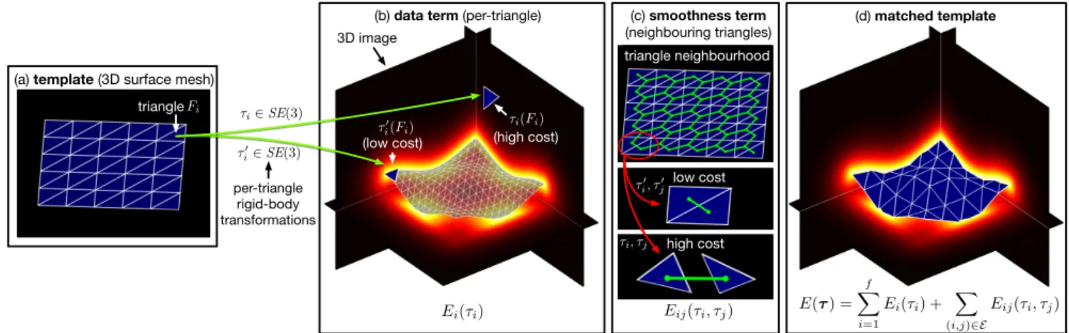
(neighbouring triangles) per-triangle rigid-body transformations 3D image (low cost) ⌧0 i2SE(3) Eij(⌧i, ⌧j) Ei(⌧i) triangle neighbourhood low cost high cost ⌧0 i, ⌧j0 ⌧i, ⌧j Fi triangle ⌧i2SE(3) (high cost) ⌧i(Fi) ⌧0 i(Fi) E(⌧) = f X i=1 Ei(⌧i) + X (i,j)2E Eij(⌧i, ⌧j)
Figure 1. 3D Shape-to-Image Matching. (a) Given a shape as a triangular mesh, we associate to each triangleFiits rigid transformation
τi ∈SE(3)such that the sum of data and smoothness terms is minimised. (b) The data termEi(τi)measures how well the transformed triangleτi(Fi)fits into the volumetric image. (c) The smoothness termEij(τi, τj)penalises the discrepancy between transformed triangles
τi(Fi)andτj(Fj). (d) OptimisingEprovides us with a shape-to-image matching.
Abstract
We propose a combinatorial solution for the problem of non-rigidly matching a 3D shape to 3D image data. To this end, we model the shape as a triangular mesh and al-low each triangle of this mesh to be rigidly transformed to achieve a suitable matching to the image. By penalising the distance and the relative rotation between neighbour-ing triangles our matchneighbour-ing compromises between image and shape information. In this paper, we resolve two major challenges: Firstly, we address the resulting large and NP-hard combinatorial problem with a suitable graph-theoretic approach. Secondly, we propose an efficient discretisation of the unbounded 6-dimensional Lie groupSE(3). To our knowledge this is the first combinatorial formulation for non-rigid 3D shape-to-image matching. In contrast to ex-isting local (gradient descent) optimisation methods, we ob-tain solutions that do not require a good initialisation and that are within a bound of the optimal solution. We evalu-ate the proposed method on the two problems of non-rigid 3D shape-to-shape and non-rigid 3D shape-to-image regis-tration and demonstrate that it provides promising results.
1. Introduction
Matching a shape template to an image is a well stud-ied problem in computer vision and image analysis. It gives rise to a wide range of applications, including image seg-mentation and object detection. An early approach for the detection of lines and parametrised curves in images is the voting-based Hough transform [14], which was later gener-alised to the detection of arbitrary shapes [1].
Whilst the Hough transform considers rigid shapes, the utilisation of shape information in image segmentation tasks has also been addressed in the non-rigid case, including methods based on active shape models [10], level sets [12], convex shape spaces [13], multiphase graph cuts [58], or statistical shape models [19, 63]. For the reconstruction of the shape of an object from a single 2D image, shape-from-template approaches aim to match a given 3D tem-plate to the image via a 3D-to-2D projection [50,38,46]. Several authors have considered combinatorial formulations of the non-rigid shape-to-image matching problem for
cer-tain classes of shapes. For the case of matching contours [11,53], or 2D chordal graph polygons [16], the resulting optimisation problems can be solved globally. However, a generalisation of these methods to 3D shapes is non-trivial and we are not aware of previous work addressing this issue. The purpose of this work is to fill this gap by presenting a combinatorial formulation for the non-rigid matching of a 3D shape template to a 3D image. For that, we model the shape as a triangular mesh and allow each triangleFiof this
mesh to be independently transformed via a rigid transfor-mationτi∈SE(3). Using a discretisation of the unbounded
6-dimensional Lie groupSE(3), we formulate the matching
task as a manifold-valued multi-labelling problem that can be cast as minimising the energy
E(τ) = n X i=1 Ei(τi) + X (i,j)∈E Eij(τi, τj). (1)
Here, the data termEi(τi)takes the image information into
account, while the smoothness term Eij(τi, τj) measures
the dissimilarity between the observed shape and the mod-elled shape prior. By penalising the distance and the rel-ative rotation of neighbouring triangles our matching com-promises between image and shape information. In general, minimising functions of the form in (1) is NP-hard [26].
1.1. Related Work
To the best of our knowledge the present paper is the first one that considers a combinatorial formulation of the non-rigid 3D shape to 3D image matching problem. In the following we will summarise methodologies that are most relevant to our work.
Continuous Optimisation: In many scenarios it is
nat-ural to assume that image or shape deformations are spa-tially continuous and smooth. Frequently, such problems are formulated in terms of optimisation problems over the space of diffeomorphisms [15,40,2,41]. Commonly, gra-dient descent-like methods are used to obtain (local) optima of the (typically non-convex) problems. However, a major shortcoming of these methods is that a good initial estimate is crucial and in general there are no bounds on the opti-mality of the solution. To deal with the non-convexity of a 2D shape-to-image matching problem that is formulated in terms of optimal transport, the authors in [52] propose to use a branch and bound scheme.
Shortest Paths and Dynamic Programming: In
con-trast to the continuous local optimisation methods, many vi-sion problems can be formulated in a discrete manner such that they are amenable to solutions based on graph
algo-rithms and dynamic programming (DP) [17]. Since curves
are intrinsically one-dimensional, various curve matching formulations can also be reduced to finding a shortest-path in a particular graph. Moreover, based on a recursive
formu-lation using easier-to-solve subproblems, matching prob-lems with templates that have a tree structure can frequently be tackled by DP. For a deformable matching of an open contour to a 2D image, a global solution based on DP has been proposed in [11]. Also based on DP, in [16] the authors present a method for solving the problem of deformably matching a 2D polygon to a 2D image for chordal graph polygons. In [53], the authors propose a globally optimal approach for matching a closed contour to a 2D image based on cycles in a product graph of the contour and the image. A related formulation that is also based on a product graph has recently been introduced in [30] for deformable contour to 3D shape matching.
Graph-cuts: It is well known (see e.g. [4]) that any cut
of a graph can be interpreted as finding a closed manifold of co-dimension 1 in the ambient space (e.g., closed curve in 2D, closed surface in 3D, etc.). One such example is the reconstruction of a 3D shape from a set of sparse 3D points, where the latter is represented on a discrete 3D grid [35].
Labelling Problems: Labelling problems are
ubiqui-tous in computer vision and appear both in continuous
and discrete settings [62]. The popular Markov Random
Field (MRF) framework offers a Bayesian treatment thereof
[37]. Also, linear programming relaxations of MRFs have
been studied [59]. The continuous approaches to
multi-labelling include various convex relaxations [47, 32, 55,
18], multi-labelling problems with total variation regular-isation of functions with values on manifolds [33], as well as sublabel-accurate convex relaxations [42,31]. Among the discrete multi-labelling methods are the previously-mentioned graph-cuts, which can be used to find global solutions for certain binary labelling problems, including problems with submodular pairwise costs [25]. For a sub-class of multi-labelling problems a global solution can also be found [25]. This sub-class includes pairwise costs that are convex in terms of totally ordered labels [22]. In ad-dition, efficient algorithms for finding local optima of gen-eral multi-labelling problems have been proposed [6,27], which even have theoretical optimality guarantees. A more detailed description of the energy functions that can be op-timised using graph-cuts is given in [26,24,25].
1.2. Main Contributions
The main contribution of this paper is to present for the first time a combinatorial formulation of the non-rigid 3D shape to 3D image matching problem. Whilst our problem is a natural extension to the afore-mentioned “dimension one” matching approaches [11,16,53,30], a generalisation to (intrinsic)dimension twoproblems is more intricate. Our main contributions are:
• By using a surface mesh transformation model that
formulate the 3D shape to 3D image matching problem in terms of a manifold-valued multi-labelling problem.
• We introduce a pairwise term that defines a metric
on the label space SE(3), which itself is a
high-dimensional Lie group. With that, our energy
func-tion is amenable to be minimised by theα-expansion
algorithm [6], which has been shown to work well in practice, is efficient even for very large label spaces, and has theoretical optimality guarantees.
• In contrast to continuous optimisation methods that
use gradient descent-like algorithms, our combinato-rial method does not require a good initialisation. • In order to deal with the computationally challenging
discretisation ofSE(3), we propose to use a coarse-to-fine discretisation of the Lie group.
2. Non-Rigid 3D Shape-to-Image Matching
In this section we first specify our objective, followed by a description of the data term and smoothness term. After introducing the combinatorial problem, we describe the dis-cretisation of the label space and we discuss the algorithmic solution of the problem.2.1. Objective Function
In the following, we assume that a 3D shapeS ⊂ R3
is given as a triangular mesh. This means we haven ∈ N
trianglesF1, . . . , Fn⊂R3such that
S=
n [ i=1
Fi. (2)
We use the setE ⊂ {1, . . . , n}2to define the neighbour-hood between pairs of (different) triangles. We assume that for all(i, j) ∈ Ethe neighbouring trianglesFi andFj are
non-disjoint and that the intersectionFi∩Fjresults either
in a common edge or a common vertex. Also, w.l.o.g. we assume that for each (i, j) ∈ E it holds thati < j, i.e.
(i, j)∈ E ⇒(j, i)∈ E/ .
Our objective is it now to match the 3D shapeS onto
a volumetric imageI: Ω → Rc, whereΩ ⊂ R3 denotes
the compact image domain andc∈Ndescribes the amount
of image channels. While we are interested in a non-rigid shape-to-image matching, we like to favour matchings that are as-rigid-as-possible, similar to the approach in [54] that applies (locally regularised) rigid transformations to each vertex. However, in our case this is done by applying to each triangleFia rigid transformation
τi= (˜τi, ~τi)∈SE(3) = SO(3)n R3, (3) whereτ˜i ∈ SO(3) ⊂ R3×3 represents the rotational part and~τi ∈ R3 represents the translational part of τi. The
task of finding the best matchingτ = (τ1, . . . , τn)can be
formulated as minimising the energy
E(τ) = n X i=1 Ei(τi) + X (i,j)∈E Eij(τi, τj). (4)
In Section 2.2we define the data termEi(τi)that
evalu-ates how well the transformed triangleτi(Fi)fits to the
im-age data. In Section 2.3we define the smoothness term
Eij(τi, τj) that measures the geometric dissimilarity
be-tween the shape modelSand the transformed shape
τ(S) :=
n [ i=1
τi(Fi). (5)
Using the proposed piecewise rigid transformation model
we may end up with a modelτ(S)having (small) gaps or
intersections between neighbouring triangles. We will later address this issue and present a simple yet effective way of dealing with this irregularity.
2.2. Data Term
The data termEi(τi)∈Rmeasures how well the trans-formed triangle τi(Fi)fits to the image data I. For that,
we introduce the score imageJ : Ω → [0,1]that is
de-rived from the imageI(e.g. a gradient magnitude image, or more advanced predictors based on neural networks). For a triangleF ⊂Ω, we define
J[F] :=
Z F
J(x)dx. (6)
With that, the valueJ[F]indicates how well the triangleF
fits to the image data, where a high value of the score image indicates a good fit. The data term is then given by
Ei(τi) =−J[τi(Fi)]. (7)
In the discrete setting, the data termEi is computed by
a weighted sum of function values−J(x)over the triangle. The weights take the rasterisation of the deformed triangle
τi(Fi)in the image into account.
2.3. Smoothness Term
The pairwise termEij(τi, τj) ∈ R+0 penalises the dis-agreement between neighbouring trianglesFi andFj after
they have been transformed byτiandτj, respectively.
For defining the pairwise term we first introduce suitable distances. The expression
dSO(3)(˜τi,τ˜j) = r 1 2 log(˜τT i τ˜j) F (8)
is the geodesic distance between the rotations τ˜i and τ˜j
and qj being the quaternion representations of τ˜i andτ˜j,
one can efficiently compute the distance as dSO(3) =
2 cos−1(|hq
i, qji|), where h·,·i is the quaternion
inner-product [21].
For defining a distance between neighbouring triangles, we make use of the concept of group actions. To be more specific, we define
dSE(3),X(τi, τj) = max
x∈Xkτi(x)−τj(x)k2, (9)
where the groupSE(3)acts on the non-empty compact set
X ⊆ R3. In our case we useX = Fi ∩Fj such that
dSE(3),Fi∩Fj(τi, τj)can be seen as distance between the de-formed trianglesτi(Fi)andτj(Fj). In this case the
maxi-mum indSE(3),Fi∩Fj(τi, τj)is achieved at the common ver-tices ofFiandFj, which is attractive from a computational
point of view.
Using the introduced distances, we define our pairwise term as a weighted sum thereof,i.e.
Eij(τi, τj) = (10)
λBdSO(3)(˜τi,τ˜j) +λSdSE(3),Fi∩Fj(τi, τj).
The purpose of the bending term, weighted by λB > 0,
is to ensure that the rotations of neighbouring triangles are similar. The stretching term, weighted byλS >0, ensures
that neighbouring triangles stay close together.
2.4. Combinatorial Formulation
A matching τ of shapeS to the image Iis given by a
solution of the optimisation problem min
τ∈SE(3)n E(τ). (11)
Due to the non-convexity of the feasible setSE(3)n, it
fol-lows that Problem (11) is non-convex. This non-convexity makes it difficult to solve the problem directly over the un-bounded continuous spaceSE(3)n. Our approach is to
opti-mise instead over a discretisation of the search space. With that, we obtain a multi-labelling problem, for which effi-cient and effective algorithms are available.
For the discretisation ofSE(3)we make use of the fact that it is a product space ofSO(3)andR3. Thus, we define
L ⊂SO(3)nR3= SE(3)to be the (finite) manifold-valued label space that contains`=|L|elements ofSE(3).
Translations:The Lie groupSE(3)is non-compact due
to the translational part being encoded by R3. However,
since the image domainΩis compact, the image size
pro-vides natural bounds for a discretisation of the translations. Letnx, ny, nzbe the number of voxels of the imageIand
`x, `y, `z be the number of labels for the x, y,z
transla-tions. For convenience, and w.l.o.g., we assume that our template is defined relative to the centre of the image do-main, i.e. the template’s centre-of-gravity coincides with
the centre of the image. Moreover, w.l.o.g., we assume that we are looking for a matching such that a substan-tial part of the (transformed) template lies inside the im-age1. Let us define Z
m(n) = {−n2, . . . ,0, . . . ,n2}to be
the set containingmevenly-spaced elements with centre0,
where mis an odd positive integer. The diameter n
de-fines the difference between the largest and the smallest el-ements. A discretisation of the translations is given by the setL~ =Z`
x(nx)×Z`y(ny)×Z`z(nz)with|L|~ =`x·`y·`z.
Rotations:Various works that are related to the
discreti-sation ofSO(3)have previously been presented. These
in-clude sampling strategies for rigid-body path planning [29],
an approximation of the neighbourhood inSO(3)based on
vector distances [36], or an analysis of various metrics for 3D rotations [21]. Our discretisation ofSO(3)is based on theHopf fibration, which describesSO(3)in terms of the circleS1and the 2-sphereS2. The intuition of this approach is to transfer a discretisation ofS1andS2to the space of ro-tations. We refer the interested reader to [61] for a detailed description. LetL˜denote the so-obtained set of a uniform sampling ofSO(3)containing`˜=|L|˜ elements.
By optimisingEover the label spaceLn, we now obtain
the combinatorial optimisation problem as min
τ∈Ln E(τ). (12)
3. Algorithm
In order to solve Problem (12), we useα-expansion [6,
26, 5], which greedily updates only one label at a time.
We note that there are also potential alternatives to α
-expansion (e.g. for non-metric pairwise terms [27,55], or fusion moves [34]). Whilstα-expansion has the
require-ment that the pairwise term is a metric, it is appealing both from a practical and a theoretical point of view. To be more specific, it is efficient, robust with respect to initialisation, the obtained local optimum is guaranteed to lie within a fac-tor of the global optimum, and an efficient implementation that supports the online computation of the smoothness term is available [6,26,5], which is crucial for the size of prob-lems that we are solving. We now show that our pairwise term is a metric and thusα-expansion is applicable.
Lemma 1 LetX ⊆ R3 be a non-empty compact set and
τi, τj, τk ∈SE(3). The stretching term
dSE(3),X(τi, τj) = max
x∈Xkτi(x)−τj(x)k2, is a pseudometric,i.e. it satisfies
(i) dSE(3),X(τi, τj)≥0, dSE(3),X(τi, τi) = 0, (ii) symmetry:dSE(3),X(τi, τj) =dSE(3),X(τj, τi), and
(iii) the triangle inequality:
dSE(3),X(τi, τk)≤dSE(3),X(τi, τj)+dSE(3),X(τj, τk). Proof: (i) and (ii) follow directly from the definition. The triangle inequality holds, since
dSE(3),X(τi, τk) = max x∈Xkτi(x)−τk(x)k2 = max x∈Xkτi(x)−τk(x) +τj(x)−τj(x)k2 ≤max x∈X kτi(x)−τj(x)k2+kτj(x)−τk(x)k2 ≤max x∈Xkτi(x)−τj(x)k2+ maxx∈Xkτj(x)−τk(x)k2 =dSE(3),X(τi, τj) +dSE(3),X(τj, τk).
Proposition 1 ForλS, λB >0and(i, j)∈ E, the pairwise
termEij(·,·)defined in(10)is a metric.
Proof: Due to the assumption in Section 2.1, for(i, j) ∈
E it follows that X := Fi ∩ Fj 6= ∅ is compact.
Thus,dSE(3),X(·,·)is a pseudometric (Lemma1). Whilst
dSO(3)(·,·)is known to be a metric on SO(3), it is only a pseudometric on SE(3). Since Eij(·,·) is a positive
linear combination of two pseudometrics, Eij(·,·)is also
a pseudometric. To show that Eij(·,·) is a metric, we
show thatEij(τi, τj)=0impliesτi=τj. ForEij(τi, τj)=0,
it holds that dSO(3)(˜τi,τ˜j)=0, which implies τ˜i=˜τj.
Moreover, with Eij(τi, τj)=0 and τ˜i=˜τj, it holds that
dSE(3),X(τi, τj)= maxx∈Xk(˜τi(x)+~τi)−(˜τj(x)+~τj)k2 =
k~τi−~τjk2=0, which implies~τi=~τj. Henceτi=τj.
3.1. Coarse-to-Fine Processing
In practice, for a reasonably large number of labels`= ˜
`·`x·`y·`z, a direct solution of Problem (12) is intractable.
In order to cope with this issue we propose to use a coarse-to-fine strategy that (approximately) solves Problem (12) at different levels sof the label space. Let s=0 denote the coarsest (initial) level and s=smax ≥ 0 the finest (final) level. Once a solution τ(s) has been obtained at level s, for running the algorithm at levels+1the labelling is ini-tialised withτ(s)and the label space is updated accordingly. For computational efficiency, in the coarse-to-fine approach each triangle has its own feasible label space. LetL(is)
de-note this feasible label space for the i-th triangle at level s. Initially, on the base levels=0, the label spaces are the same for each triangle,i.e.L(0)i =L(0). The general idea for obtainingL(s+1)
i is to consider a (uniform)
discretisa-tion of the neighbourhood of the transformadiscretisa-tionτi(s)at level
s, where the radius of the neighbourhood decreases across the levels. Let us introduce a neighbourhood onSO(3):
Definition 1 (-ball onSO(3))
The ball onSO(3)with radiusand centreτ˜ ∈ SO(3)is defined asBSO(3) (˜τ) ={τ ∈SO(3) :dSO(3)(τ,τ˜)< }.
Next, we describe the coarse-to-fine structure of the label space based on its product space nature. Since each label can be written as τi(s)= (˜τ (s) i , ~τ (s) i )∈L˜ (s) i ×L~ (s) i ⊂SO(3)n R3, (13)
we can consider the translations and rotations indepen-dently. Note thatL˜(s)
i ×L~
(s)
i ⊂SE(3)is not necessarily a
group anymore. By enforcing thatτi(s) ∈ L(is+1), the solu-tionτ(s)at levelsis also contained in the new label space. Thus, the energy cannot increase from levelstos+1.
Translations: We defineL~(0) := L~ (cf. Section2.4).
For obtaining the set of translations at levels+1for triangle
i, the new translation grid at levels+1is centred at~τi(s).
Moreover, the diameter from levelsis reduced by a factor of two, leading to ~ Li(s+1):= (14) ~τi(s)+ Z`x( n(xs) 2 )×Z`y( n(ys) 2 )×Z`z( n(zs) 2 ) ! ,
where the vector-set addition is element-wise. Initially,
n(0)x =nx, n(0)y =nyandn(0)z =nz.
Rotations: LetL˜[r] denote a discretisation of (the
en-tire)SO(3)at resolutionrcontaining`˜[r] elements, where ˜
`[r] increases with increasing r. L˜[r] should not be con-fused withL˜(s)
i , which is the (rotation) label space of the
i-th triangle at levelsthat is to be defined below.
Follow-ing the construction in [61], we obtain5resolutions of the SO(3) discretisationL˜[r] forr = 0, . . . ,4. After includ-ing the identity inL˜[r], the number of elements ranges from ˜
`[0]= 577to`˜[4]≈2·106. Let us define a set that contains a fixed number ofpelements fromL˜[r]that are “closest” to the identity,i.e.
˜
L[r]
p := ˜L[r]∩ BSO(3) (Id), (15)
where for each resolution r the smallest that fulfils
|L˜[pr]| ≥pis used as radius.
Now, we defineL˜(0):= ˜L[0], and ˜
Li(s+1):={ττ˜
(s)
i :τ∈L˜[ps+1]⊆SO(3)}, (16)
which is the set of compositions ofτ˜i(s)with all rotations
in L˜[s+1]
p . We use p = ˜`[0] = 577 for all levelss. For
the predefinedSO(3)griddings at resolutionsr= 0, . . . ,4 there always existed ansuch that the above inequality is
tight,i.e.|L˜[pr]|= ˜`[0]= 577.
By including the identity in L˜[s+1]
p , we make sure that
˜
τi(s) ∈ L˜i(s+1). Since0 ∈ Z·(·), it follows that~τi(s) ∈
~
Li(s+1). Thus, we haveτ
(s)
i ∈ L
(s+1)
i , ensuring that the
3.2. Practical Considerations
In this section we describe some aspects for the applica-tion of the proposed method in practice.
3.2.1 Mesh Connectivity
After applying an individual rigid-body transformation to each triangle of the template mesh, in general the resulting mesh may have gaps or intersections between neighbouring triangles. However, due to the introduced regulariser, these gaps or intersections can be expected to be rather small. For recovering the original mesh topology, we replace each sub-set of vertices having the same position in the mesh template by their centre-of-gravity after the transformation.
3.2.2 Memory Requirements
For running our algorithm we pre-compute the data term, requiring memory of O(n·`) (the online computation has constant memory requirements but leads to a significantly increased runtime). Since pre-computing the full pairwise
term requires memory of O(n2
·`2), we only precompute the bending termdSO(3), requiring memory ofO(˜`2). The stretching termdSE(3),Xis computed online.
4. Results
For the evaluation of our method we focus on demon-strating the general applicability of our approach. Both point-set registration [3,48,8,36,44,43,23,20,49,39] and the related correspondence problem for 3D shapes [56,60,28,7] can be tackled using our method by recasting them as shape-to-image matching problem. Hence, in our evaluation below, in addition to 3D image segmentation, we also consider the case of deformable mesh registration.
4.1. Deformable Mesh Registration
In the first set of experiments we demonstrate that our method can be used to perform deformable mesh registra-tion. To emphasise that our method is insensitive to initial-isation, we compare it exemplarily with the Coherent Point Drift (CPD) algorithm [44,43], a widely-used point-cloud registration method based on Expectation Maximisation.
Template and Target:For the evaluation we use a
low-resolution mesh of the Stanford bunny as template (n =
498), as shown in Fig.2(top left). A total of20deformed versions of the bunny mesh, each with a random pose, are used as registration targets. For that, we synthetically create deformed versions of a high-resolution bunny mesh (Fig.2, top right) based on random 3D displacement vectors defined at8control points on a cubic grid. These displacement vec-tors are then transferred to the mesh using a spline-based
interpolation in order to achieve a smooth and nonlinear de-formation. One such deformed mesh is shown in Fig.2 (bot-tom left). Eventually, a random pose transform is applied to the deformed shape, as shown in Fig.2(bottom right).
Figure 2. Bunny meshes. Top left: template. Top right:
high-resolution target. Bottom left: deformed target (with original tar-get overlay). Bottom right: deformed tartar-get with random pose.
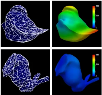
Figure 3. Qualitative results for registrations of the bunny
tem-plate to the deformed target with random pose (cf. Fig.2, bottom right). Top left: CPD result (shape destroyed). Top right: CPD error. Bottom left: our result. Bottom right: our error.
Score Image: In order to use our method for mesh
registration we create a score image for each target mesh and then fit the template mesh to the score image. For
d : Ω → R+0 we denote byd(x)the distance of position
xto the boundary of the target mesh. Now, we define the
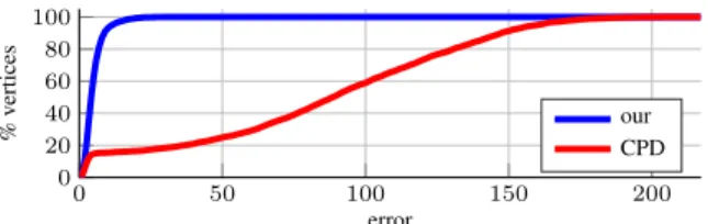
0 50 100 150 200 0 20 40 60 80 100 error % vertices our CPD
Figure 4.Percentage of vertices (vertical axis) which have an error
that is smaller than or equal to the value on the horizontal axis.
Parameters: We set λS = 54·max({nxg,ny,nz}) and
λB = 27·πg, where the normalisation factor g = nc2|E|max
takes the problem size into account. The positive num-ber cmax is an upper bound for the largest possible abso-lute value of the data term for a single triangle (cf. eq. (6)), which we compute by multiplying the largest value of the score image by the area of the largest triangle. The size of the label space is|L(0)
| = 93
·577 = 420,633, and the
dimensions of the score image range from2083 to 2623,
which resulted in an average processing time of≈92
min-utes per registration on a MacBook Pro (2.5GHz, 16GB).
Results: In the case of CPD, we first solve for a
rigid registration and then for a non-rigid registration (per-forming a non-rigid registration directly performed worse). Since CPD is highly initialisation-sensitive it fails in17out of the20evaluated cases, where one representative failure case is depicted in Fig.3(top row). This extreme amount of corrupt registrations emphasises the necessity of a method that is robust with respect to initialisation. In contrast, in all 20cases our method is able to achieve a good registration, see Fig.3(bottom row) for a representative result. In Fig.4 we present a quantitative evaluation.
Discussion: Whilst we do not claim to present an
exhaustive evaluation of mesh registration methods, we demonstrated the insensitivity to initialisation of our method in a proof of concept manner. One advantage of our approach is that we neither have the necessity of com-patible mesh topologies, nor of comcom-patible mesh discreti-sations, since the target is represented in terms of the score image. Since the score image is a discrete representation of the target shapesurface, our approach amounts to a surface-based registration, rather than a point-surface-based registration as CPD, which is biased towards aligning points to be as close as possible. Moreover, the score image offers further flex-ibility since additional information can be integrated (e.g. uncertainties, mesh texture, shape features, etc.).
4.2. Segmentation
In the second set of experiments we apply our method to the segmentation of four brain structures (substantia ni-gra & subthalamic nucleusas single object and thenucleus ruber, both bilaterally) in16multi-modal3T magnetic
res-onance images. The delineation of thesubthalamic nucleus
is known to be a challenging task, even for humans [51].
The main difficulties include weak image contrasts and the small size of the brain structures (the structures shown in Fig.5are contained in a bounding box of≈6×3×2.5cm3, with the MRI image covering a volume of≈203cm3).
Template: For capturing the inter-relation between the
brain structures, we use a multi-object template (n=379), as
shown in Fig.5. The template connects neighbouring brain
structures by (degenerate) triangles, referred to as “phantom triangles”, which are used only for the smoothness term and are “free” with respect to the data term.
Figure 5.Brain structure template.
Parameters: We set λS = 135·max({nxg,ny,nz}) and
λB = 90·πg, wheregis defined as before. The size of the
label space is|L(0)
|= 113
·577 = 767,987, and the dimen-sion of all score images is364×436×364, which resulted in an average processing time of≈58minutes per fitting.
Score Image: In order to perform image segmentation
with our method, we use a data term that is based on the
re-cently proposed 3D U-Net CNN [9]. For all16images we
train the network in a leave-one-out manner for the predic-tion of volumetric segmentapredic-tions. In the centre column of Fig.7three examples of so-predicted volumetric segmenta-tions are shown. For this challenging segmentation task the U-Net is able to identify the (rough) location of the brain structures, but does in many cases not produce an output that resembles the shape of the brain structures (the first two
rows in Fig.7). Thus, we complement the U-Net
segmenta-tions with geometric information using our method. For each of the four brain structureso∈ {1,2,3,4}we use an individual score imageJo. Given the binary U-Net
segmentation Iounet : Ω → {0,1}for brain structureo, we
first extract the (predicted) boundary using morphological operations. For do : Ω → R+0 we denote by do(x)the
distance of positionxto the so-extracted boundary. Then,
we use a Gaussian kernel to define the score image as
Jo(x) =woexp −−d 2 o(x) 2σ2 o . (17)
The weightwoand bandwidthσoare used for incorporating
the confidence about the U-Net segmentationIounetof brain
structureo. To this end, for
being the one-level set of Iounet that represents the
point-cloud of segmented voxels, we use the average of the
(per-coordinate) median absolute deviation (MAD) as robust
dispersionmeasure, computed as MAD(Yo) =
1
3kMAD(Yo)k1, (19)
for MAD(Yo) = median(|Yo−median(Yo)|) ∈ R3. The median is understood in a per-coordinate sense, and both the set-vector difference and the absolute value are
un-derstood element-wise. Now, for Y0
o denoting the
point-cloud of segmented voxels of structure oas given by the
template, the absolute value of the average MAD difference is given byho =|MAD(Yo)−MAD(Yo0)|. With that, we
defineσo = ρ(ho+1), scaled byρ=3. Thus, if the
aver-age MAD for the U-Net segmentation and the template are equal, the bandwidth corresponds toρ, whereas a larger dif-ference in dispersion leads to a larger bandwidth, account-ing for more uncertainty in the U-Net segmentation. More-over, we definewo = ho1+1 such that an increased
uncer-tainty in the U-Net segmentation of brain structureoleads
to a decreased weight for its data term.
Results: For the evaluation of the segmentation we use
the Dice Similarity Coefficient (DSC) as volumetric overlap measure, which is defined as 2|Y∩Y0
|
|Y|+|Y0|, forY andY0 each being point-clouds of segmented voxels. We compute the DSC for each individual brain structure, and then report the average of the four DSC values. Quantitative results com-paring the plain U-Net segmentation and our obtained seg-mentations are presented in Fig.6. The boxplot on the left reveals that in overall our method achieves higher volumet-ric overlaps across the16cases. Moreover, the plot of sorted DSC differences on the right emphasises that applying our method improves the DSC in most cases (the values above zero), and in only a few cases it is reduced slightly. In Fig.7
our unet 0.2
0.4 0.6
DSC
best median worst
0 0.2 0.4 DSC our − DSC unet
Figure 6.Left: Boxplot of the DSC of our method versus the
U-Net segmentation. Right: Sorted DSC differences for the16cases
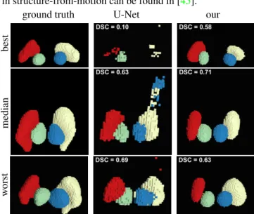
(values above zero indicate an improvement upon U-Net). qualitative results for three segmentation cases that corre-spond to thebest,medianandworstcases in Fig.6(right) are shown. In the first row of Fig.7it can be seen that in some cases our method is even able to achieve a reasonable segmentation based on a poor U-Net segmentation. This was possible by putting a stronger emphasis on the shape information relative to the data term, which also biases the
method towards the shape information. A related discus-sion on the biasedness of model-to-data fitting approaches in structure-from-motion can be found in [45].
ground truth U-Net our
best
median
w
orst
Figure 7. Qualitative results for the brain structure segmentation
experiments. Each row shows a different instance of results, where from top to bottom we present thebest, medianandworstDSC
differences (cf. Fig.6, right).
5. Conclusion
We introduced the first combinatorial method for non-rigidly matching a 3D shape to a 3D image. The key idea is to represent the 3D shape as a triangular mesh and to solve a manifold-valued multi-labelling problem on the set of triangles. We determine an assignment of a rigid-body transformation associated with each triangle by minimis-ing a cost function where the unary terms encode the local matching cost in the image and the pairwise terms penalise the amount of non-rigidity in the deformation. In particu-lar, we propose an efficient discretisation of the unbounded 6-dimensional Lie group of rigid motions. Moreover, we solve the large and NP-hard optimisation problem with a graph theoretic algorithm that is insensitive to initialisation and has the guarantee that the obtained solution is within a factor of the global optimum [6]. Experimental validation confirms these benefits.
Acknowledgements
The authors would like to thank ¨Ozg¨un C¸ic¸ek for help-ful feedback regarding the U-Net implementation, as well as Benedikt Staffler and Ankush Gupta for general feed-back on CNNs. CNN-related computations presented in this paper were carried out using the HPC facilities of the
University of Luxembourg [57]. The authors gratefully
acknowledge the financial support by the Fonds National de la Recherche, Luxembourg (6538106, 8864515). This work was supported by the ERC Consolidator Grant 3D Reloaded.
References
[1] D. H. Ballard. Generalizing the Hough transform to detect arbitrary shapes.Pattern Recognition, 13(2):111–122, 1981.
1
[2] M. F. Beg, M. I. Miller, A. Trouv´e, and L. Younes. Comput-ing large deformation metric mappComput-ings via geodesic flows of diffeomorphisms.International Journal of Computer Vision,
61(2):139–157, 2005.2
[3] P. J. Besl and N. D. McKay. A method for registration of 3-D shapes.TPAMI, 14(2):239–256, 1992.6
[4] Y. Boykov and V. Kolmogorov. Computing Geodesics and Minimal Surfaces via Graph Cuts.ICCV, 2003.2
[5] Y. Boykov and V. Kolmogorov. An experimental comparison of min-cut/max-flow algorithms for energy minimization in vision.TPAMI, 26(9):1124–1137, 2004.4
[6] Y. Boykov, O. Veksler, and R. Zabih. Fast approximate en-ergy minimization via graph cuts. TPAMI, 23(11):1222–
1239, 2001.2,3,4,8
[7] Q. Chen and V. Koltun. Robust Nonrigid Registration by Convex Optimization.ICCV, 2015.6
[8] H. Chui and A. Rangarajan. A new point matching algo-rithm for non-rigid registration.Computer Vision and Image Understanding, 89(2):114–141, 2003.6
[9] ¨O. Cicek, A. Abdulkadir, S. S. Lienkamp, T. Brox, and O. Ronneberger. 3D U-Net: Learning Dense Volumetric Seg-mentation from Sparse Annotation. InMICCAI, 2016.7
[10] T. F. Cootes and C. J. Taylor. Active Shape Models - Smart Snakes. InBMVC, pages 266–275, 1992.1
[11] J. Coughlan, A. Yuille, C. English, and D. Snow. Efficient deformable template detection and localization without user initialization. Computer Vision and Image Understanding,
78(3):303–319, 2000.2
[12] D. Cremers. Dynamical statistical shape priors for level set-based tracking.TPAMI, 28(8):1262–1273, 2006.1
[13] D. Cremers, F. R. Schmidt, and F. Barthel. Shape priors in variational image segmentation: Convexity, lipschitz conti-nuity and globally optimal solutions. InCVPR, 2008.1
[14] R. O. Duda and P. E. Hart. Use of the Hough transformation to detect lines and curves in pictures.Communications of the ACM, 15(1):11–15, 1972.1
[15] P. Dupuis, U. Grenander, and M. I. Miller. Variational problems on flows of diffeomorphisms for image matching.
Quarterly of applied mathematics, pages 587–600, 1998.2
[16] P. F. Felzenszwalb. Representation and detection of de-formable shapes.TPAMI, 27(2):208–220, 2005.2
[17] P. F. Felzenszwalb and R. Zabih. Dynamic Programming and Graph Algorithms in Computer Vision. TPAMI, 33(4):721–
740, 2011.2
[18] B. Goldluecke, E. Strekalovskiy, and D. Cremers. Tight con-vex relaxations for vector-valued labeling.SIAM Journal on Imaging Sciences, 6(3):1626–1664, 2013. 2
[19] T. Heimann and H.-P. Meinzer. Statistical shape models for 3D medical image segmentation: A review. Medical Image Analysis, 13(4):543–563, 2009.1
[20] R. Horaud, F. Forbes, M. Yguel, G. Dewaele, and J. Zhang. Rigid and articulated point registration with expectation
con-ditional maximization. TPAMI, 33(3):587–602, Mar. 2011.
6
[21] D. Q. Huynh. Metrics for 3D Rotations: Comparison and Analysis. Journal of Mathematical Imaging and Vision,
35(2):155–164, June 2009.3,4
[22] H. Ishikawa. Exact optimization for Markov random fields with convex priors.TPAMI, 25(10):1333–1336, 2003.2
[23] B. Jian and B. C. Vemuri. Robust Point Set Registration Us-ing Gaussian Mixture Models. TPAMI, 33(8):1633–1645,
2011.6
[24] V. Kolmogorov and Y. Boykov. What Metrics Can Be Approximated by Geo-Cuts, Or Global Optimization of Length/Area and F.ICCV, 2005.2
[25] V. Kolmogorov and C. Rother. Minimizing non-submodular functions with graph cuts – a review. TPAMI, 29(7):1274–
1279, 2007.2
[26] V. Kolmogorov and R. Zabih. What energy functions can be minimized via graph cuts? TPAMI, 26(2):147–159, Feb.
2004.2,4
[27] N. Komodakis and G. Tziritas. Approximate labeling via graph cuts based on linear programming. TPAMI,
29(8):1436–1453, 2007.2,4
[28] A. Kovnatsky, M. M. Bronstein, X. Bresson, and P. Van-dergheynst. Functional correspondence by matrix comple-tion. InCVPR, 2015.6
[29] J. J. Kuffner. Effective sampling and distance metrics for 3D rigid body path planning . InICRA, Jan. 2004.4
[30] Z. L¨ahner, E. Rodol`a, F. R. Schmidt, M. M. Bronstein, and D. Cremers. Efficient Globally Optimal 2D-to-3D De-formable Shape Matching.CVPR, 2016.2
[31] E. Laude, T. M¨ollenhoff, M. M¨oller, J. Lellmann, and D. Cre-mers. Sublabel-Accurate Convex Relaxation of Vectorial Multilabel Energies.ECCV, 2016.2
[32] J. Lellmann and C. Schn¨orr. Continuous multiclass label-ing approaches and algorithms. SIAM Journal on Imaging Sciences, 4(4):1049–1096, 2011. 2
[33] J. Lellmann, E. Strekalovskiy, S. Koetter, and D. Cremers. Total variation regularization for functions with values in a manifold. InICCV, 2013.2
[34] V. Lempitsky, C. Rother, S. Roth, and A. Blake. Fu-sion moves for markov random field optimization. TPAMI,
32(8):1392–1405, 2010.4
[35] V. S. Lempitsky and Y. Boykov. Global Optimization for Shape Fitting.CVPR, 2007.2
[36] H. Li and R. Hartley. The 3D-3D Registration Problem Re-visited. InICCV, 2007.4,6
[37] S. Z. Li.Markov random field modeling in computer vision.
Springer Science & Business Media, 2012.2
[38] A. Malti, A. Bartoli, and R. Hartley. A Linear Least-Squares Solution to Elastic Shape-From-Template.CVPR, 2015.1
[39] H. Maron, N. Dym, I. Kezurer, S. Kovalsky, and Y. Lip-man. Point registration via efficient convex relaxation.ACM Transactions on Graphics (TOG), 35(4):73, 2016.6
[40] P. W. Michor and D. Mumford. Riemannian Geometries on Spaces of Plane Curves. InJournal of the European Mathe-matical Society, 2004.2
[41] M. I. Miller, A. Trouv´e, and L. Younes. Geodesic shooting for computational anatomy.Journal of Mathematical Imag-ing and Vision, 24(2):209–228, 2006.2
[42] T. M¨ollenhoff, E. Laude, M. Moeller, J. Lellmann, and D. Cremers. Sublabel-Accurate Relaxation of Nonconvex Energies. InCVPR, 2016.2
[43] A. Myronenko and X. Song. Point Set Registration: Coher-ent Point Drift.TPAMI, 32(12):2262–2275, Dec. 2010.6
[44] A. Myronenko, X. Song, and M. A. Carreira-Perpin´an. Non-rigid point set registration: Coherent Point Drift. InNIPS,
2007.6
[45] I. Nurutdinova and A. Fitzgibbon. Towards Pointless Struc-ture from Motion: 3D Reconstruction and Camera Parame-ters from General 3D Curves. InICCV, 2015.8
[46] S. Parashar, D. Pizarro, A. Bartoli, and T. Collins. As-Rigid-as-Possible Volumetric Shape-from-Template. ICCV, 2015.
1
[47] T. Pock, T. Schoenemann, G. Graber, H. Bischof, and D. Cre-mers. A convex formulation of continuous multi-label prob-lems. InECCV, 2008.2
[48] A. Rangarajan, H. Chui, and F. L. Bookstein. The softassign procrustes matching algorithm. InIPMI, 1997.6
[49] A. Rasoulian, R. Rohling, and P. Abolmaesumi. Group-wise registration of point sets for statistical shape models. TMI,
31(11):2025–2034, Nov. 2012.6
[50] M. Salzmann and P. Fua. Reconstructing sharply folding sur-faces: A convex formulation. InCVPR, 2009.1
[51] J. R. Schlaier, C. Habermeyer, J. Warnat, M. Lange, A. Janzen, A. Hochreiter, M. Proescholdt, A. Brawanski, and C. Fellner. Discrepancies between the MRI- and the elec-trophysiologically defined subthalamic nucleus. Acta Neu-rochirurgica, 153(12):2307–2318, July 2011. 7
[52] B. Schmitzer and C. Schn¨orr. Globally optimal joint im-age segmentation and shape matching based on Wasser-stein modes. Journal of Mathematical Imaging and Vision,
52(3):436–458, 2015.2
[53] T. Schoenemann and D. Cremers. A combinatorial solution for model-based image segmentation and real-time tracking.
TPAMI, 32(7):1153–1164, 2010.2
[54] O. Sorkine and M. Alexa. As-rigid-as-possible surface mod-eling.Symposium on Geometry Processing, 2007.3
[55] E. Strekalovskiy, B. Goldl¨ucke, and D. Cremers. Tight con-vex relaxations for vector-valued labeling problems. ICCV,
2011.2,4
[56] O. Van Kaick, H. Zhang, G. Hamarneh, and D. Cohen Or. A survey on shape correspondence. InComputer Graphics Forum, pages 1681–1707, 2011.6
[57] S. Varrette, P. Bouvry, H. Cartiaux, and F. Georgatos. Man-agement of an academic hpc cluster: The ul experience. In
Proc. of the 2014 Intl. Conf. on High Performance Comput-ing & Simulation (HPCS 2014), 2014.8
[58] N. Vu and B. S. Manjunath. Shape prior segmentation of multiple objects with graph cuts. InCVPR, 2008.1
[59] T. Werner. A linear programming approach to max-sum problem: A review.TPAMI, 29(7):1165–1179, 2007.2
[60] T. Windheuser, U. Schlickewei, F. R. Schmidt, and D. Cre-mers. Geometrically consistent elastic matching of 3D shapes: A linear programming solution.ICCV, 2011.6
[61] A. Yershova, S. Jain, S. M. LaValle, and J. C. Mitchell. Gen-erating Uniform Incremental Grids on SO(3) Using the Hopf Fibration. The International journal of robotics research,
29(7):801–812, June 2010.4,5
[62] C. Zach, C. Hane, and M. Pollefeys. What is optimized in convex relaxations for multilabel problems: Connecting discrete and continuously inspired map inference. TPAMI,
36(1):157–170, 2014.2
[63] S. Zhang, Y. Zhan, M. Dewan, J. Huang, D. N. Metaxas, and X. S. Zhou. Sparse shape composition: A new framework for shape prior modeling. InCVPR, 2011.1