Assessing the Federal Deduction for State and Local Tax Payments

(1)

ECONOMICS DEPARTMENT

WORKING PAPER

2008

Department of Economics

Tufts University

Medford, MA 02155

(617) 627-3560

http://ase.tufts.edu/econ

(2)

Assessing the Federal Deduction for State and Local Tax Payments Gilbert E. Metcalf Department of Economics Tufts University and NBER May 6, 2008 Abstract

Federal deductibility for state and local taxes constitutes one of the largest tax expenditures in the federal budget and provides a significant source of federal support to state and local governments. Deductibility was restricted in the Tax Reform Act of 1986 by removing the deduction for general sales taxes. More recently the President's

Advisory Panel on Federal Tax Reform recommended eliminating the deduction altogether as one of several revenue-raising initiatives to finance comprehensive tax reform.

I carry out a number of distributional analyses – considering both variation across income and across states – of the subsidy from deductibility as well as the distributional impact of potential partial reforms. In addition, I consider three counterfactuals for 2004 – a tax system without the Bush tax cuts for 2001 and 2003, a tax system without the 2004 AMT patch, and a tax system without the AMT – to see how the benefits of deductibility are affected by these changes in the tax law.

Next I consider how behavioral responses affect the tax expenditure estimates. Feldstein and Metcalf (1987) argued that tax expenditures overestimate the revenue gain from eliminating deductibility as they do not take into account a likely shift away from once-deductible taxes to non-deductible taxes and fees in the absence of deductibility. Many of these latter taxes and fees are paid by businesses. As business costs rise, federal business tax collections would fall, offsetting some of the gains of ending deductibility. Feldstein and Metcalf also found that ending deductibility would have little if any impact on state and local spending itself. Using a large panel of data on state and local

governments, I revisit this issue and find that the Feldstein-Metcalf results are robust to adding more years of analysis.

* * *

This paper was prepared for the NBER Conference on Incentive and

Distributional Consequences of Tax Expenditures, held at the Hyatt Regency Coconut Point Hotel in Bonita Springs, FL on March 28-29, 2008. I am grateful for help with TAXSIM calculations from Dan Feenberg, for expert RA work from Yoshiyuki Miyoshi, and for helpful comments from Roger Gordon and other conference participants.

(3)

I. Introduction

One of the most valuable deductions on the individual income tax return is the deduction for state and local income and property taxes. Taking all state and local tax deductions as a group, the deduction is second only to the deduction for mortgage interest on owner occupied homes in aggregate importance for individual taxpayers (Office of Management and Budget (2008)). This deduction has come under attack at various times despite its widespread popularity. The most serious threat came in the run-up to the Tax Reform Act of 1986. While the elimination of the entire deduction for state and local taxes was proposed, TRA86 only removed the deduction for general sales taxes. And this curtailment was undone to some extent in the American Jobs Creation Act of 2004 when the option was allowed to deduct either income or sales taxes.1 This deduction came under scrutiny again by President George W. Bush's Advisory Panel on Federal Tax Reform. The panel argued that ending this deduction would contribute to a "cleaner and broader tax base" and a tax system that was more equitable across income groups.2

While the Panel's recommendations remain to be taken up by Congress, this deduction has been eroded to some extent by two features of the federal tax code. First, limitations on itemized deductions reduce the value of this deduction for some

households with large amounts of itemized deductions. Second, the Alternative Minimum Tax (AMT) targets this deduction directly. In fact, a major determinant of whether a taxpayer becomes subject to the AMT is the presence of large deductions for state and local taxes. A taxpayer facing the AMT loses this deduction.

1

This primarily benefitted those states with a general sales tax but no income tax: Florida, Nevada, South Dakota, Tennessee, Texas, Washington, and Wyoming.

2

(4)

The magnitude of the tax expenditure for state and local tax deductions makes it a prime target for policy makers looking for revenue to pay for other changes in the tax code.3 Feldstein and Metcalf (1987), however, argued that estimates of the revenue gain from eliminating deductibility were too high as they did not take into account a likely shift away from once-deductible taxes to non-deductible taxes and fees in the absence of deductibility. Many of these latter taxes and fees are paid by businesses. As these costs rise, federal business tax collections would fall, offsetting some of the gains of ending deductibility. Feldstein and Metcalf also found that ending deductibility would have little if any impact on state and local spending itself.

Given the interest in changing or eliminating this subsidy, I present a number of distributional analyses – considering both variation across income and across states – of the subsidy from deductibility. In particular I show that eliminating the deduction or curtailing it adds progressivity to the federal income tax. In addition, I consider three counterfactuals for 2004 – a tax system without the Bush tax cuts for 2001 and 2003, a tax system without the 2004 AMT patch, and a tax system without the AMT – to see how the benefits of deductibility are affected by these changes in the tax law. Then I consider how behavioral changes affect the tax expenditure estimates. Using a large panel of data on state and local governments, I revisit this issue and find that the Feldstein-Metcalf results are robust to adding more years of analysis.

The regressive nature of the subsidy combined with its inability to stimulate overall state and local spending makes a strong case for removing the deduction. One might make a case for the subsidy on the grounds that it serves as a type of commodity subsidy for certain state and local services that could be optimal in a world with

3

Congressional Budget Office (2008) provides a good history of this deduction and efforts to change it over time. It also carries out a number of distributional analyses similar in spirit to those in this paper.

(5)

limitations on the ability to tax labor income sufficiently flexibly (the general case for violating production efficiency is given in Stiglitz (1982) and Naito (1999)). Whether the institutional restrictions on income tax design are sufficient to support a subsidy to state and local taxes is not entirely clear. Saez (2004), however, argues that in the long-run production efficiency can be restored in models where it appears that commodity taxes or subsidies are part of an optimal tax system. Thus it is difficult to find support for this deduction on equity or efficiency grounds

II. Background

The deduction for state and local taxes is a significant form of federal aid to state and local governments. In the most recent budget submission, the deductions for all non-business state and local taxes amounts to nearly $50 billion in FY2009, making it the fifth largest tax expenditure in the federal budget (Office of Management and Budget (2008)). While state and local tax deductibility dates to the creation of the modern income tax, it became a major focus of research activity in the mid-1980s when President Ronald Reagan proposed to eliminate the deduction as part of the first tax reform proposal in late 1984. The final legislation, The Tax Reform Act of 1986, ultimately eliminated the deduction for general sales taxes. Many felt that this was not especially controversial as most taxpayers used sales tax look-up tables which, from an individual taxpayer's point of view, did not necessarily appear related to their own spending.

Early research on this topic focused on the role that deductibility played in encouraging state and local spending. After all, one of the rationales for the deduction is to support spending at the sub-national level that might have significant spillover effects into other jurisdictions. Spending on public parks, for example, by one community might benefit members of other communities who could enjoy the park. In other words, state

(6)

and local spending could have important positive externalities or be public goods. In the absence of federal intervention, it was argued that state and local governments were unlikely to provide the optimal amount of these goods and services.4 Early papers in this literature include Noto and Zimmerman (1983, (1984), and Ladd (1984). Attention was increasingly paid to the mix of taxes chosen as well as the level of spending.

Zimmerman (1983) provided a median voter analysis of the relationship of income tax reliance on deductibility while Hettich and Winer (1984) provided a political economy analysis. Neither paper was successful at finding a economically sensible relationship between deductibility and tax reliance.

Feldstein and Metcalf (1987) employed an average voter framework to analyze the impact of deductibility on state and local spending and tax reliance. Their innovation was to use the IRS Public Use Files with the NBER's tax calculator, TAXSIM, to

estimate average marginal tax prices for state and local deductible taxes. Based on a cross-section of states, they found little evidence that own-source spending was affected by deductibility but did find that the mix of tax instruments was influenced by the deduction. Subsequent work by Holtz-Eakin and Rosen (1986), Metcalf (1993), and Gade and Adkins (1990) corroborated the findings of Feldstein and Metcalf using different time periods, and various combinations of state and local governments.5

Figure 1 shows the state and local tax expenditure for non-business taxes excluding the property tax in real dollars (1982-84). The tax expenditure drops off sharply after 1986 with the drop in marginal tax rates following TRA86. It then has

4

Whether state and local government goods and services are public goods or provide positive externalities is a question I do not address in this paper.

5

Feldstein and Metcalf's results suggested that states would shift away from their reliance on general sales taxes after 1986. This appeared not to happen. A number of papers addressed this issue including Inman (1989), Courant and Gramlich (1990), Metcalf (1992), and Metcalf (1993). More recent work by Izraeli and Kellman (2003) suggests that reliance on the general sales tax did eventually fall once sufficient time had passed.

(7)

increased steadily until the Bush tax cuts enacted in 2001 and 2003. A similar pattern is observed for the tax expenditure for state and local property taxes (Figure 2). Figure 3 scales the tax expenditures for state and local taxes by state and local own-source

revenue. Again the pattern holds of a decline in the ratio after 1986 followed by a steady increase until this decade. Figure 4 shows two key determinants of the level of tax expenditures. It measures the ratio of state and local taxes to personal income and the national average marginal tax rate on wage income as computed by TAXSIM. The sharp decline in marginal tax rates after TRA86 explains the sharp fall in tax expenditures in 1987. The gradual increase in the share of state and local taxes in personal income along with the rise in marginal tax rates contributes to the growth in tax expenditures. This trend stops with the sharp fall in marginal tax rates beginning in 2001.

III. Measuring the Revenue Loss from State and Local Tax Deductibility

Before considering any behavioral responses that might arise from ending deductibility, I provide some statistics on measurements of the tax expenditure for deductibility where behavioral responses are ignored. I first focus on errors that arise from adding tax expenditure estimates. Both OMB and the Joint Committee on Taxation report tax expenditure estimates for state and local tax deductibility separately. In

general, users are cautioned not to add tax expenditure estimates given interactions within the tax code as deduction and other tax expenditure items are changed. For example, one might expect that eliminating the deduction for all state and local personal taxes would yield a smaller tax expenditure estimate than the sum of the tax expenditures for personal non-property taxes and property taxes since removing one of the deduction will push some taxpayers below the threshold for itemizing deductions at which point their other state and local tax deduction becomes worthless. On the other hand, removing one tax

(8)

deduction could push taxpayers into higher tax brackets thereby making the other deduction more valuable. Thus whether summing individual tax expenditures over or underestimates the tax expenditure estimate from removing both deductions is a priori uncertain.

The first row of Table 1 shows results from using TAXSIM to estimate the state and local tax deduction tax expenditures for calendar year 2004 using the SOI public use file assuming elimination of the deduction under current law. This is the difference in tax liability for an individual return (as calculated by TAXSIM) between the current law and the law assuming the elimination of the deduction. This difference is computed at the individual level and then aggregated using the weight from the SOI dataset. The sum of the individual estimates underestimates the aggregate measure by less than one-half of one percent. This suggests that adding the two estimates does not seriously misrepresent the estimate of the tax expenditure from ending both deductions simultaneously.6 Figure 5 shows this error over time. It peaks at 5 percent in 1993 and has been steadily falling since.

I also consider the errors in adding the tax expenditure estimates under different assumptions about the tax law. In the second row of Table 1, I assume that no AMT patch is applied in 2004. Now adding the estimates underestimates the aggregate tax expenditure estimate by 8 percent. The error is smaller if the AMT is eliminated

altogether or the Bush tax cuts not in effect. In either case the error is less than 5 percent. In short, it does not appear that large errors occur when adding tax expenditure estimates

6

At the taxpayer level, adding expenditure estimates overestimates the tax expenditure by at least $580 for one percent of returns and underestimates the tax expenditure by at least $700 for one percent of returns. The error for ninety percent of taxpayers is $104 or less. The error is less than one-half of one percent of cash income for over 98 percent of filers.

(9)

for the two state and local tax deduction tax expenditures to get an estimate of the tax expenditure arising from eliminating all state and local tax deductions altogether.

Next I provide estimates of tax expenditures for other changes to this deduction and consider the interaction between the federal tax treatment of state and local tax payments and the Bush tax cuts as well as the AMT. In particular, I consider three other reforms. The first replaces the deduction with a 15 percent non-refundable tax credit. In effect this allows all taxpayers to deduct their state and local taxes as if they were in the 15 percent tax bracket.7 The second reform caps the deduction. I consider two caps: one where all taxes are subject to a cap of $5,000 per year and a second where the cap is set equal to 3.5 percent of AGI. The third reform allows a deduction above a floor. If policymakers believe that the tax deduction has positive incentive effects, the floor lowers the cost of providing the deduction while continuing to provide an incentive for state and local spending. Like the cap, I provide two types of floors: one set at $7,575 and a second set at 4.4 percent of AGI. The two caps and floors are constructed to generate a tax expenditure of $35 billion in 2004. Results are shown in Table 2.

The first column of Table 2 shows the revenue cost under current law of taking intermediate actions rather than entirely eliminating the deduction for state and local taxes. Replacing the deduction with a 15 percent tax credit raises considerably less than eliminating the deduction in part because taxpayers who were not receiving the benefit of the deduction due to their taking the standard deduction now have the opportunity to take

7

I calculate state income taxes for non-itemizers using the TAXSIM state tax calculator. For property taxes, I hot deck from the Consumer Expenditure Survey. I draw a similar taxpayer from the CEX (based on income category and number of dependents) and check to see if the taxpayer would itemize using the mortgage interest and property tax deduction imputed from the CEX (along with the calculated state income tax deduction). If this return would itemize, I discard the CEX household and draw another similar household. If this return would not itemize, I use this household's property tax payment for the SOI taxpayer.

(10)

the credit. As noted above, the cap and floor reforms all have a tax expenditure of $35 billion under current law.

Table 2 also shows the interaction between the deduction and other tax code provisions. If there had been no AMT patch in 2004, the tax expenditure associated with eliminating deductibility would have been reduced by $10 billion, roughly 15 percent. The next column shows clearly how the AMT reduces the value of deductibility raising the tax expenditure by nearly $10 billion. The AMT reduces the value of the state and local tax deduction considerably. In the absence of an AMT patch, imposing the AMT reduces the value of the deduction by over one-quarter. Finally, the Bush tax cuts also reduced the value of the deduction substantially with a reduction for 2004 of roughly 20 percent. Unlike the AMT, however, the value of the deduction is reduced not by

disallowing the deduction but rather by lowering marginal tax rates. A similar pattern holds for the alternatives to eliminating deductibility.

IV. Distributional Analysis

How are the benefits of deductibility distributed across taxpayer groups? In this section, I report both income and geographic measures of the benefits of the deduction. For the income analysis, I use cash income to sort taxpayers. Cash income equals adjusted gross income less state and local tax refunds plus adjustments to income, MSA and Keogh deductions, tax-exempt interest and non-taxable Social Security benefits. The distributional impact is measured by taking weighted averages across the 150,000 returns in the 2004 Public Use File at different income deciles.8

8

Cut-offs for the deciles in cash income are $5,440, $11,365, $17,340, $23,898, $31,960, $41,730, $53,710, $70,831, and $100,973. The 95th percentile cut-off is $140,381 and the 99th percentile cut-off is $343,872.

(11)

Table 3 presents the change in average tax liability for different income groups if deductibility were eliminated. The increase in average tax liability is below $100 for the bottom 60 percent of the income distribution. The tenth decile faces an average increase of $3,238. Considerable skew occurs in this top decile as evidenced by the mean

exceeding the increase in tax liability for the 75th percentile. Breaking down the top decile a bit further, the largest increases occur in the top one percent of the distribution. As a percentage of cash income, the increase in tax liability is quite small – less than one percent for the bottom 90 percent of the income distribution. Eliminating this deduction does add progressivity to the tax system as the liability as a percentage of cash income rises monotonically with income. The last column of Table 3 shows that the share of returns facing higher taxes goes up steadily with income.

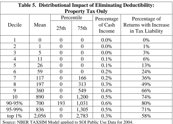
A second reform possibility is to eliminate deductibility for a subset of state and local taxes. Table 4 and 5 provide distributional impacts of these reforms. More revenue is collected (ignoring behavioral responses) by eliminating the deduction for income and personal property taxes than property taxes. Moreover, eliminating the income and personal property tax deductions adds more progressivity to the tax code than does eliminating the property tax deduction.

As an alternative to eliminating deductibility altogether, I consider three possibilities: replacing the deduction with a 15 percent tax credit; placing a cap on deductions; and allowing deductions above a floor. Table 6 provides distributional results for shifting from the current deduction to the 15 percent credit. This reform raises substantially less revenue than other reforms in part because households who take the standard deduction are allowed to take the credit. Thus this reform lowers tax liability for some households though as Table 6 indicates the reductions are quite modest. Fewer

(12)

taxpayers face higher tax bills than occurs if deductibility is eliminated altogether and the average change in tax liability is less than one-half of one percent of cash income. Compared to eliminating deductibility, this reform is less progressive.

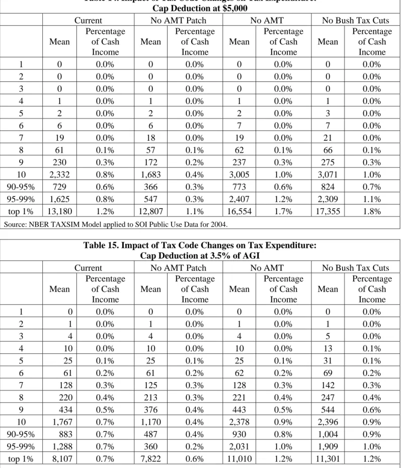
Deductions can be capped in several ways. I present results for a $5,000 cap and a cap set at 3.5 percent of AGI. The tax expenditure estimate for both of these reforms is $35.0 billion in 2004. Tables 7 and 8 illustrate the trade-offs in the two approaches. The dollar based cap reform is more progressive than the AGI percentage cap reform.

Capping the deduction as a percentage of AGI increases the tax liability more for the lower 90 percent of the income distribution than capping the deduction at $5,000. The AGI based cap, however, leads to lower tax increases than does the dollar based cap for the top 5 percent of the income distribution.

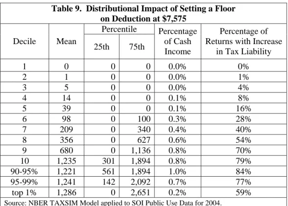
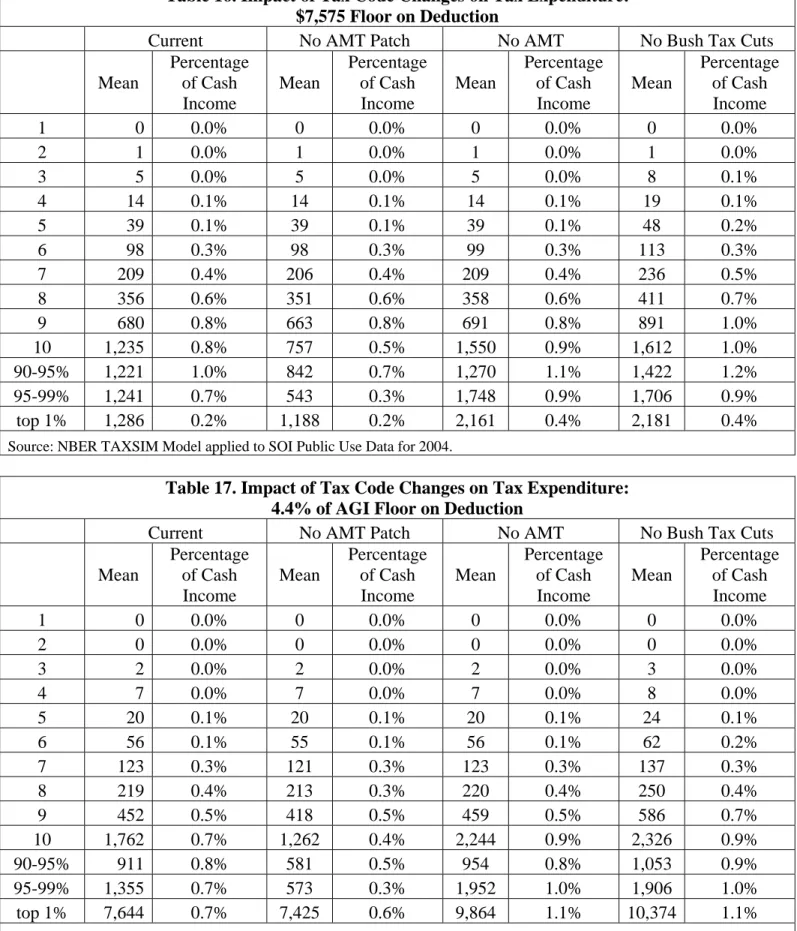
Allowing a deduction above a floor is analyzed in Tables 9 and 10. In contrast to the cap approach, the dollar based floor reform is less progressive than the AGI

percentage based floor reform. Comparing the dollar based cap and floor, the cap reform is more progressive than the floor reform. The dollar based floor approach preserves an incentive gain for state and local spending at the cost of some progressivity. The AGI approach comparison is more mixed. Except for the top 1 percent of the distribution, the floor reform is more progressive than the cap reform.

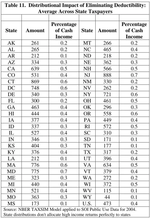
Table 11 presents some distributional information across states. This table reports the average increase in tax liability by state from eliminating deductibility in dollar terms and as a percent of income. The average increase per return in the U.S. is $473. Several states have increases in excess of $700 (NJ, CT, MA, MD, DC, NY) while other states see average increases of less than $200 (TN, MS, SD, WV, WY). On a percentage basis,

(13)

NJ, MD, CT, MA, DC, NY, and OR have increases of 0.6 percent of income or more while AR, LA, TN, MS, SD, WV have increases that are 0.1 percent of income.

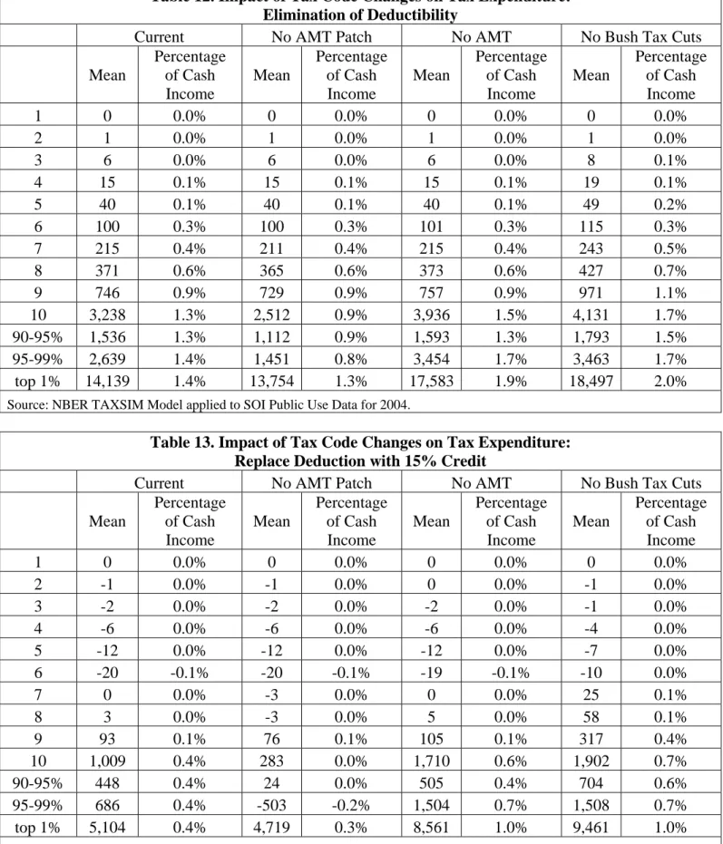
Tables 12 through 17 consider how changes in the tax code affect the distribution of tax expenditures for various reform proposals. In Table 12, I consider eliminating all deductions for state and local taxes assuming no AMT patch, no AMT, and no Bush tax cuts, all in 2004. The pattern of increased taxes from eliminating the deduction is not surprising given the aggregate estimate of the tax expenditure in Table 1. A few interesting facts emerge. First, the AMT patch in 2004 increases the regressivity of the deduction with most of the impact occurring in the top decile. This point is reinforced by a comparison of the Current distribution with the No AMT distribution. In the absence of the AMT the state and local tax deduction is more regressive, again with nearly all the increased regressivity occurring in the top 5 percent of the income distribution. Second, the Bush tax cuts also served to reduce the regressivity of this deduction. Unlike in the AMT case, the change in tax burden is spread over more deciles. Similar patterns occur for the other potential reforms of the deduction.

These distributional results hold behavior constant. I next turn to a

reconsideration of the behavioral impacts of ending deductibility of state and local taxes. While the results from this analysis can't be used to compute new distributional tables, they are informative about the revenue impact of ending or otherwise modifying deductibility.

V. Empirical Analysis of Behavioral Response to the Deduction

State and local governments choose their mix of revenue instruments as well as the level of spending knowing that taxpayers in their state may be able to deduct some of these taxes on their federal return. This exporting of state and local taxes to the federal

(14)

government lowers the political cost of raising revenue at the sub-federal level. How do state and local governments respond to this feature of the federal tax code? I measure this response by following the empirical strategy of Feldstein and Metcalf (1987) and estimating regressions of state and local deductible taxes, non-deductibletaxes, and own-source revenue where I control for the impact of federal deductibility. In contrast to this previous analysis, I employ panel data from 1979 through 2001, excluding 2000.9

Where calendar year data are matched with fiscal year data, the calendar year data for the beginning of the fiscal year are used. Thus for state and local data for FY 1998, calendar year data from 1997 are used. This reflects the fact that decisions about fiscal structure are set at the beginning of the fiscal year which occurs in the previous calendar year.

The key tax variable is the tax price for state and local tax deductions. This is the reduction in federal and state taxes arising from an additional dollar of tax deduction. As a simple example of the concept, consider a taxpayer whose federal tax bracket is 25 percent. Further assume that federal taxes are not deductible at the state level. In that case, an additional $100 of state tax deductions will reduce federal tax liability by $25. The net cost of raising this $100 of state taxes is only $75 as $25 has been exported to the federal government through deductibility. If mi is the ith taxpayer's federal marginal tax

bracket, then this taxpayer's tax price (Pi) for state and local deductible taxes is

(1) Pi = 1 – mi.

This assumes that the taxpayer itemizes her deductions. The tax price for a non-itemizer is one. Let di be a dummy variable equally one for an itemizer and zero for a

non-itemizer. Then this taxpayer's tax price is

9

State and local fiscal data are from the Bureau of the Census, Federal, State, and Local Governments webpage at http://www.census.gov/govs/www/estimate.html. Data were accessed in July, 2007. State level data are not available for FY 2000.

(15)

(2) Pi = di(1-mi) + (1-di) = 1 – dimi.

If federal taxes can be deducted at the state level, then the formula for the tax price is slightly more complicated:

(3)

(

)

_S

(

)

i F i F i S i S i F i i m m m m m m P − − + − − = 1 1 1 1 .

While this is a formidable looking equation, the NBER's TAXSIM calculator can compute these tax prices easily. TAXSIM is a computer tax model of the federal and state tax codes covering federal and state tax codes from 1977 to 2006.10

I estimate regressions of the following form:

(4) Y_it =β₁P_it +X_itβ₂ +α_i +γ_t +ε_it

where i indexes states and t indexes years. The dependent variable is some function of deductible state and local taxes, non-deductible state and local taxes and fees, or own source revenue. I will report regressions where the dependent variable is the fiscal

variable relative to personal income or the log of the fiscal variable. In the latter case, the log of income is included as a regressor. The 1 by k vector, Xit, contains variables that

help explain the dependent variable. These must vary within states over time given the inclusion of state-specific fixed effects and year dummies. State-specific fixed effects are included to control for unobserved attributes of a state that affect fiscal structure and are likely correlated with explanatory variables.11 Year dummies provide a flexible

framework for controlling for aggregate shocks to state and local tax systems and spending.

10

See Feenberg and Coutts (1993) for a description of TAXSIM. Equation (3) is not exactly correct as it does not account for the phase out of itemized deductions that began in 2000 or the Alternative Minimum Tax. TAXSIM takes these provisions of the tax code into account when computing tax prices.

11

See Holtz-Eakin (1986) for a discussion of biases arising from not controlling for fixed effects in state and local government fiscal structure regressions.

(16)

As pointed out by Feldstein and Metcalf (1987), OLS regressions run on equation (4) are likely to provide biased estimates of the coefficient on the tax price variable. This is most easily seen by considering equation (2). Consider a shock that increases state income tax collections. This increases the deduction available to the tax payer with two opposing effects. The first effect is that an increase in the potential state tax deduction increases the likelihood that a taxpayer will itemize on her federal tax return. This

induces a negative correlation between the error term (ε_it) and the tax price Pit and biases

the OLS estimate of β1 down. The second effect is that an increase in deductions could

push the tax payer into a lower tax bracket lowering mit. This induces a positive

correlation between the error term and the tax price and biases the OLS estimate of β₁ up. Which effect dominates is an empirical question.

To control for endogeneity, I construct three instruments. The first is a synthetic instrument that attributes to each household the national probability of itemizing based on number of dependents (0, 1, 2+) and AGI group. I divide households into one of eight equally sized AGI groups.12 The instrument for taxpayer i in year t is

(5) dˆit(Depit = j,AGI Classit =k)=dtN(j,k)

where dNt(j, k) is the probability of itemizing in the national sample in year t for

households with j dependents in AGI class k.

The second instrument is constructed by setting the ith taxpayer's state and local tax deductions to zero and computing the change in tax liability resulting from a marginal increase in wage income. Call this marginal tax rate m_it0. The instrument is called a first dollar tax price and equals

12

(17)

(6) Pit0 =1−dˆitmit0.

The third instrument is constructed by replacing the taxpayer's state and local tax deductions with national averages based on number of dependents and AGI class and then computing the change in tax liability resulting from a marginal increase in wage income. Call this marginal tax rate m_itL. The last dollar tax price equals

(7) P_itL =1−dˆ_itm_itL.

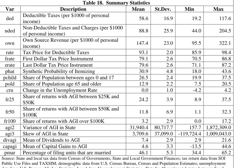
Table 18 shows summary statistics for the variables I use in the regressions. Deductible taxes average 5.8 percent of personal income, ranging from 1.9 to 11.8 percent. Nondeductible taxes and fees average 8.9 percent of personal income and show a wider range across states and time. Own source revenue is the sum of these two

variables averaging 14.7 percent of personal income. In addition to the tax price variable, I include demographic data on percentage young (age 17 and under) and old (age 65 and older). These two demographic groups are important drivers of demands for state and local public services, especially at the local level.13 The change in the unemployment rate is included to control for state-specific economic shocks not captured by state or year effects. The next set of variables captures features of the distribution of income in the state that could affect the demand for revenue as well as the tax mix. They also control for non-linear income effects that the tax price variable might otherwise be proxying for. Finally, I include information about the share of households married in the state.

Table 19 presents regression results for personal deductible taxes. Column (1) presents an OLS regression of non-business deductible taxes on the tax price variable and other control variables. Before discussing the tax price coefficient, let me discuss some

13

It is possible that state tax structure can affect the age distribution of populations living in a state. This is an interesting issue that I do not pursue in this paper. I thank Roger Gordon for pointing this out. Tax price results are insensitive to excluding these variables.

(18)

of the other variables. The coefficient on the AGI range variables are positive with the coefficient on fr25 and fr100 statistically significant. As might be expected the

coefficient on fr100 is substantially larger than the coefficient on fr25 or fr50. This pattern holds in general for the other regressions on non-business deductible taxes. The AGI variance and skew variables never come in statistically significant in these

regressions indicating that once controlling for shares of AGI in various income groups, other distribution statistics do not affect the choice of these taxes. The form of income also has little impact on the level of this tax. The coefficient on capagi is statistically significant in all regressions though the estimated elasticity (not reported) is quite small.

States with a large share of young children or elderly people tend to have lower reliance on personal deductible taxes though only the coefficient on the share of young children is statistically significant. The coefficient on the elderly share likely reflects a demand for lower overall spending by the elderly. The coefficient on the child share is a bit puzzling since this should correlate with a demand for school spending. Contrary to the finding in Metcalf (1993), increases in the unemployment rate are associated with a greater reliance on personal deductible taxes.

The coefficient on the tax price variable equals -2.57 and is highly statistically significant. The elasticity at the mean equals -4.1 suggesting that tax structure is highly responsive to changes in the tax price. We must be cautious about this estimate given the potential endogeneity discussed above. The next regression in Table 19 presents two stage least squares estimates of the coefficients controlling for the endogeneity in the tax price variable with the instruments described above. The first stage regression (not reported here) has a high R2 with an F statistic on the joint significance of the instruments highly significant. In the second stage regression (column (2)) the coefficient estimate on

(19)

the tax price variable increases in absolute value from -2.57 to -2.72. The upward bias in the OLS estimate suggests that the tax bracket bias outweighs the itemization bias. While the coefficient is less precisely estimated, it is still statistically significant at the 1 percent level. The elasticity at the mean of the reliance on deductible taxes with respect to the tax price is -4.3.

The next regression excludes other explanatory variables except for the AGI share variables, the change in unemployment rate and the population demographic variables. The two stage least squares estimate rises slightly from -2.72 to -2.84 and continues to be highly statistically significant.14 The tax price elasticity at the mean from this regression equals -4.5. As in all other two-stage least squares regressions that I run, the first stage regressions fit quite well and provide no evidence of problems arising from weak instruments.

I also report regressions for a log specification where the dependent variable is the ln of deductible taxes. In addition to the AGI share variables, I include the log of income in the regression. The tax price coefficient in the two-stage least squares regressions continues to have the expected sign but is not statistically significant in the full regressors specification and only significant at the 10 percent level in the restricted specification and the elasticity of revenues with respect to the tax price is lower than the elasticity implied by the levels regressions.

The pattern of results from the levels and log regressions are quite similar to the those of Feldstein and Metcalf (1987). The levels regressions tend to suggest higher

14

Which variables I choose to exclude has little impact on the coefficient estimates. If I drop all variables except the year dummies, the estimated tax price coefficient equals -4.70 with a standard error of 0.52. If I drop all other variables including the year dummies, the estimated tax price coefficient rises to -5.90 with a standard error of 0.20. Excluding year effects likely biases the coefficient estimate down. Adverse aggregate shocks reduce state income tax revenue and are likely to push taxpayers into lower tax brackets thereby raising their tax price.

(20)

elasticities at the means and have a higher level of statistical significance than the coefficients arising from the log regressions.15

If changes in the tax mix occur in response to changes in the deductibility of state and local taxes, then we should see an increase in the use of non-deductible taxes and fees in response to an increase in the tax price for state and local taxes. I explore this in Table 20. The format of the table is the same as Table 19. Column (1) presents results from an OLS regression using the full set of explanatory variables. The coefficient on the tax price variable is positive as would be expected if tax shifting from deductible taxes to non-deductible taxes and fees were occurring but the coefficient estimate is not

statistically significant. The AGI share variables suggest that states with a large share of tax filers with AGI of at least $100,000 rely less on non-deductible taxes and fees, a result consistent with the results in Table 19 and quite plausible given the higher value of the deduction to high tax-bracket filers.

Once I instrument for the tax price variable (column (2)), the coefficient on this variable increases to 2.34 and is statistically significant at the 5 percent level. As in the OLS regression, states with a high share of high income households tend to prefer deductible to non-deductible taxes with the coefficient on fr100 substantially larger in this regression. The elasticity at the mean for the tax price variable is 2.46 confirming the finding from the Table 19 regressions that tax swapping is quite sensitive to changes in the tax price for state and local tax deductions. Using the restricted set of regressors, the coefficient estimate rises to 3.04 and continues to be highly statistically significant. Now the elasticity at the mean is 3.2. The log regressions also confirm the tax shifting result

15

One might be concerned that my AGI distribution variables do not entirely control for income effects and that the tax price variable continues to pick up some income effects. Income is explicitly included in the log regressions. I experimented with adding AGI to the ratio regressions and the results are not affected.

(21)

though the two-stage least squares estimate with the full set of regressors is only statistically significant at the 10 percent level. For the regression with restricted set of regressors, the p-value of the coefficient estimate is .04.

Tables 19 and 20 have focused on how state and local governments choose their mix of taxes and fees. I now turn to the impact of deductibility on own source revenue. The first column of Table 21 reports an OLS regression of the ratio of own source revenue to personal income on the full set of regressors. By this regression, the

deduction leads to a substantial increase in reliance on own source revenue by state and local governments. However, the result goes away once I instrument for the tax price variable (column (2)). The estimated coefficient on the tax price variable is -0.38 but not statistically significant. Of the other variables, the demographic variables have the most substantial impact. States with a higher share of elderly, in particular, have substantially lower levels of own source revenue. The elasticity at the means for this regressor equals -0.55 and is the largest elasticity among all the regressors in this specification.

Results are robust to the specification form. Restricting the regressors in the levels regression changes the point estimate on the tax price variable to 0.20 but it is still not statistically significant. The regression estimate is negative in both log specifications but again neither large nor statistically significant.

Summarizing, deductibility appears to have little impact on the overall level of own source revenue at the state and local level. But it does appear to have an effect on the mix of revenues with a greater reliance on the income and personal property tax and lesser reliance on non-deductible taxes and fees.

The Treasury tax expenditure estimate for state and local tax deductibility equaled $65 billion in fiscal year 2004. Let's consider the implications of the regression estimates

(22)

for eliminating deductibility in that year. The average marginal tax price for deductible taxes in calendar year 2003 was 94.3. Consider the regression estimates from the ratio regression with restricted number of regressors. This implies that removing deductibility will reduce deductible taxes per thousand dollars of personal income by 2.8 times the change in tax price. Nondeductible taxes and charges per thousand dollars of personal income are predicted to rise by 3.0 times the change in tax price. Finally own-source revenue per $1000 of personal income is predicted to rise by 0.2 times the change in tax price. Personal income in calendar year 2003 was $9.15 trillion. The regression

estimates imply that removing deductibility leads to a reduction in deductible taxes of $146 billion. Non-deductible taxes and fees increase by $156 billion and own-source revenue rises by $10 billion.

The increase in non-deductible taxes and fees more than offsets the decline in deductible taxes. If these non-deductible taxes and fees were entirely paid by corporate businesses, then corporate income tax collections would fall by $55 billion, 84 percent of the value of the tax expenditure arising from removing deductibility. This assumes a 35 percent rate applied to these increased taxes and fees. The calculation does not factor in any lost tax revenues from reductions in dividends paid or capital gains. It also does not allow for the possibility that some of the cost is shifted to workers in the form of lower wages or consumers in the form of higher prices. In the former case, the relevant tax rate would be that on wage earnings while if the latter, no revenue loss occurs.16

16

I also computed revenue losses from the restricted log regressions (last columns of Tables 19-21). The impacts on deductible taxes, non-deductible taxes and fees, and own-source revenue from ending

deductibility are not internally consistent across the three regressions since the log of own-source revenue is not equal to the sum of the logs of the two revenue sources. If I assume that the impact on own-source revenue is zero (the own-source regression predicts a $6 billion fall, a decline of less than one-half of one percent), I can estimate the revenue impact either from the regression in Table 19 or Table 20. Using the estimate from the deductible tax regression, the offset from corporate tax collections (assuming businesses pay the entire increase in non-deductible taxes and fees) is $30 billion, just under half the reported tax

(23)

In reality not all of the non-deductible taxes are paid by corporations. It can not be determined from an inspection of the components of these taxes and fees what the burden would be on corporate taxable income from a removal of deductibility. Current collections reflect the average burden. What determines the revenue loss is the marginal change in tax instruments arising from an end to deductibility. But regardless, it appears that the tax expenditure estimate that ignores the behavioral response at the state and local level leads to quite possibly a substantial overestimate of the revenue benefits of eliminating deductibility.

VI. Conclusion

The deduction for state and local taxes has been in the income tax since its modern inception. It is justified by some proponents as an important subsidy for state and local spending on the grounds that it increases spending on public goods that would otherwise be underfunded. While I do not assess the argument that state and local government spending is on public goods and therefore likely to be underfunded, the empirical evidence is that the tax deduction does not lead to increased state and local spending. In fact the empirical evidence is mixed with some estimates suggesting more spending and others less. None of the IV estimates, however, are statistically significant.

The evidence is compelling, however, that deductibility affects the mix of revenue instruments chosen at the state and local level. Deductibility leads to a greater reliance on income and property taxes and a lower reliance on non-deductible taxes and fees. Because these non-deductible taxes and fees are a cost for businesses, some of the revenue that would arise from eliminating this deduction would be lost through declines

expenditure loss from ending deductibility. If I use the estimate from the regression in Table 20, the offset is $107 billion, roughly two-thirds larger than the estimated tax expenditure.

(24)

in corporate and business tax income. The revenue loss offset to the measured tax expenditure could be quite substantial.

Distributional analysis suggests that the tax deduction is quite regressive. Moreover the value of the subsidy varies considerably across states. Alternatives to eliminating this deduction that I considered include capping the deduction, setting a floor on the deduction, and replacing it with a 15 percent tax credit. The cap and floor reforms are intermediate options that raise about one-half the revenue that is raised by eliminating the deduction (ignoring behavioral offsets). Replacing the deduction with a 15 percent tax credit raises the least amount of revenue before behavioral responses since some people are now eligible for the credit who take the standard deduction and so do not benefit from the deduction. In terms of adding progressivity to the tax code, the tax credit has at best a modest impact in large part due to the smaller amount of revenue raised under this reform. Capping the deduction as a percentage of AGI is less progressive than capping it with a dollar based cap. In contrast, the AGI percentage based floor reform is more progressive than a dollar based floor reform.

This paper has shown that the tax system can be made more progressive if the deduction for state and local taxes is eliminated or curtailed. The regression results also suggest that the deduction is ineffective at increasing own source spending at the sub-federal level. It may be that the deduction encourages a shift in spending from certain programs to other areas. This remains an interesting topic for future research.

(25)

Table 1. Tax Expenditure Estimates: CY 2004 Proposal Personal, Non-Property Taxes Property Taxes All Deductible Taxes Adding Error Current Law 40,330 22,014 62,549 -0.3% No AMT Patch 32,063 16,391 52,587 -7.9% No AMT 48,617 26,602 71,987 4.5%

No Bush Tax Cuts 52,024 28,293 78,860 1.8%

Source: NBER TAXSIM Model applied to SOI Public Use Data for 2004. All amounts are in millions of dollars.

Table 2. Effects of Tax Law Changes on Tax Expenditure Estimates

Proposal Current Law No AMT Patch No AMT No Bush Tax Cuts Eliminate Deductibility 62,546 52,585 71,985 78,859 15% Tax Credit 14,062 4,093 23,553 30,128 $5,000 Cap on Deduction 35,063 25,628 44,071 45,537

3.5% AGI Cap on Deduction 35,025 26,234 43,263 45,589

$7,575 Floor on Deduction 34,897 28,208 39,230 44,135

4.4% AGI Floor on Deduction 34,909 27,745 41,406 44,925

Source: NBER TAXSIM Model applied to SOI Public Use Data for 2004. All amounts are in millions of dollars.

(26)

Table 3. Distributional Impact of Eliminating Deductibility: All State and Local Taxes

Percentile Decile Mean 25th 75th Percentage of Cash Income Percentage of Returns with Increase

in Tax Liability 1 0 0 0 0.0% 0% 2 1 0 0 0.0% 1% 3 6 0 0 0.0% 4% 4 15 0 0 0.1% 8% 5 40 0 0 0.1% 16% 6 100 0 100 0.3% 28% 7 215 0 342 0.5% 40% 8 371 0 627 0.6% 54% 9 746 0 1,196 0.9% 70% 10 3,238 840 3,191 1.3% 86% 90-95% 1,536 609 2,289 1.3% 85% 95-99% 2,639 1,209 3,814 1.4% 89% top 1% 14,139 1,915 13,254 1.4% 84%

Source: NBER TAXSIM Model applied to SOI Public Use Data for 2004.

Table 4. Distributional Impact of Eliminating Deductibility: Income and Personal Property Tax Only

in Tax Liability 1 0 0 0 0.0% 0% 2 0 0 0 0.0% 0% 3 1 0 0 0.0% 1% 4 5 0 0 0.0% 4% 5 16 0 0 0.1% 11% 6 47 0 0 0.1% 21% 7 109 0 149 0.2% 30% 8 197 0 351 0.3% 42% 9 432 0 729 0.5% 58% 10 2,244 0 1,961 0.8% 70% 90-95% 903 0 1,471 0.8% 70% 95-99% 1,531 0 2,433 0.8% 70% top 1% 11,794 0 10,577 1.0% 69%

(27)

Table 5. Distributional Impact of Eliminating Deductibility: Property Tax Only

in Tax Liability 1 0 0 0 0.0% 0% 2 1 0 0 0.0% 1% 3 5 0 0 0.0% 3% 4 11 0 0 0.1% 6% 5 26 0 0 0.1% 13% 6 59 0 0 0.2% 24% 7 117 0 166 0.2% 36% 8 197 0 313 0.3% 49% 9 360 0 549 0.4% 66% 10 890 0 1,200 0.5% 74% 90-95% 700 193 1,031 0.6% 80% 95-99% 836 0 1,305 0.5% 71% top 1% 2,056 0 2,783 0.3% 58%

Table 6. Distributional Impact of Replacing Deduction with 15% Tax Credit

in Tax Liability 1 0 0 0 0.0% 0% 2 -1 0 0 0.0% 0% 3 -2 0 0 0.0% 0% 4 -6 0 0 0.0% 0% 5 -12 0 0 0.0% 0% 6 -20 0 0 -0.1% 2% 7 0 0 0 0.0% 13% 8 3 0 0 0.0% 16% 9 93 0 276 0.1% 36% 10 1,009 0 1,189 0.4% 71% 90-95% 448 0 881 0.4% 70% 95-99% 686 0 1,507 0.4% 73% top 1% 5,104 -114 6,198 0.4% 66%

(28)

Table 7. Distributional Impact of Capping Deduction at $5,000 Percentile Decile Mean 25th 75th Percentage of Cash Income Percentage of Returns with Increase

Table 8. Distributional Impact of Capping Deduction at 3.5 Percent of AGI Percentile Decile Mean 25th 75th Percentage of Cash Income Percentage of Returns with Increase

(29)

Table 9. Distributional Impact of Setting a Floor on Deduction at $7,575 Percentile Decile Mean 25th 75th Percentage of Cash Income Percentage of Returns with Increase

in Tax Liability 1 0 0 0 0.0% 0% 2 1 0 0 0.0% 1% 3 5 0 0 0.0% 4% 4 14 0 0 0.1% 8% 5 39 0 0 0.1% 16% 6 98 0 100 0.3% 28% 7 209 0 340 0.4% 40% 8 356 0 627 0.6% 54% 9 680 0 1,136 0.8% 70% 10 1,235 301 1,894 0.8% 79% 90-95% 1,221 561 1,894 1.0% 84% 95-99% 1,241 142 2,092 0.7% 77% top 1% 1,286 0 2,651 0.2% 59%

Table 10. Distributional Impact of Setting a Floor on Deduction at 4.4% of AGI Percentile Decile Mean 25th 75th Percentage of Cash Income Percentage of Returns with Increase

(30)

Table 11. Distributional Impact of Eliminating Deductibility: Average Across State Taxpayers

State Amount Percentage of Cash Income State Amount Percentage of Cash Income AK 261 0.2 MT 266 0.2 AL 265 0.2 NC 465 0.4 AR 212 0.1 ND 218 0.2 AZ 334 0.3 NE 362 0.3 CA 639 0.5 NH 566 0.5 CO 531 0.4 NJ 888 0.7 CT 869 0.6 NM 330 0.2 DC 748 0.6 NV 262 0.2 DE 340 0.3 NY 721 0.6 FL 300 0.2 OH 461 0.5 GA 463 0.4 OK 296 0.3 HI 444 0.4 OR 558 0.6 IA 377 0.4 PA 449 0.4 ID 337 0.3 RI 572 0.5 IL 527 0.4 SC 310 0.3 IN 346 0.3 SD 171 0.1 KS 404 0.3 TN 177 0.1 KY 376 0.4 TX 317 0.2 LA 212 0.1 UT 396 0.4 MA 776 0.6 VA 634 0.5 MD 775 0.7 VT 379 0.4 ME 323 0.3 WA 272 0.2 MI 440 0.4 WI 372 0.5 MN 521 0.4 WV 115 0.1 MO 363 0.3 WY 44 0.1 MS 173 0.1 U.S. 473 0.4

Source: NBER TAXSIM Model applied to SOI Public Use Data for 2004. State distributions don't allocate high income returns perfectly to states

(31)

Table 12. Impact of Tax Code Changes on Tax Expenditure: Elimination of Deductibility

Current No AMT Patch No AMT No Bush Tax Cuts

Mean Percentage of Cash Income Mean Percentage of Cash Income Mean Percentage of Cash Income Mean Percentage of Cash Income 1 0 0.0% 0 0.0% 0 0.0% 0 0.0% 2 1 0.0% 1 0.0% 1 0.0% 1 0.0% 3 6 0.0% 6 0.0% 6 0.0% 8 0.1% 4 15 0.1% 15 0.1% 15 0.1% 19 0.1% 5 40 0.1% 40 0.1% 40 0.1% 49 0.2% 6 100 0.3% 100 0.3% 101 0.3% 115 0.3% 7 215 0.4% 211 0.4% 215 0.4% 243 0.5% 8 371 0.6% 365 0.6% 373 0.6% 427 0.7% 9 746 0.9% 729 0.9% 757 0.9% 971 1.1% 10 3,238 1.3% 2,512 0.9% 3,936 1.5% 4,131 1.7% 90-95% 1,536 1.3% 1,112 0.9% 1,593 1.3% 1,793 1.5% 95-99% 2,639 1.4% 1,451 0.8% 3,454 1.7% 3,463 1.7% top 1% 14,139 1.4% 13,754 1.3% 17,583 1.9% 18,497 2.0%

Table 13. Impact of Tax Code Changes on Tax Expenditure: Replace Deduction with 15% Credit

Mean Percentage of Cash Income Mean Percentage of Cash Income Mean Percentage of Cash Income Mean Percentage of Cash Income 1 0 0.0% 0 0.0% 0 0.0% 0 0.0% 2 -1 0.0% -1 0.0% 0 0.0% -1 0.0% 3 -2 0.0% -2 0.0% -2 0.0% -1 0.0% 4 -6 0.0% -6 0.0% -6 0.0% -4 0.0% 5 -12 0.0% -12 0.0% -12 0.0% -7 0.0% 6 -20 -0.1% -20 -0.1% -19 -0.1% -10 0.0% 7 0 0.0% -3 0.0% 0 0.0% 25 0.1% 8 3 0.0% -3 0.0% 5 0.0% 58 0.1% 9 93 0.1% 76 0.1% 105 0.1% 317 0.4% 10 1,009 0.4% 283 0.0% 1,710 0.6% 1,902 0.7% 90-95% 448 0.4% 24 0.0% 505 0.4% 704 0.6% 95-99% 686 0.4% -503 -0.2% 1,504 0.7% 1,508 0.7% top 1% 5,104 0.4% 4,719 0.3% 8,561 1.0% 9,461 1.0%

(32)

Table 14. Impact of Tax Code Changes on Tax Expenditure: Cap Deduction at $5,000

Mean Percentage of Cash Income Mean Percentage of Cash Income Mean Percentage of Cash Income Mean Percentage of Cash Income 1 0 0.0% 0 0.0% 0 0.0% 0 0.0% 2 0 0.0% 0 0.0% 0 0.0% 0 0.0% 3 0 0.0% 0 0.0% 0 0.0% 0 0.0% 4 1 0.0% 1 0.0% 1 0.0% 1 0.0% 5 2 0.0% 2 0.0% 2 0.0% 3 0.0% 6 6 0.0% 6 0.0% 7 0.0% 7 0.0% 7 19 0.0% 18 0.0% 19 0.0% 21 0.0% 8 61 0.1% 57 0.1% 62 0.1% 66 0.1% 9 230 0.3% 172 0.2% 237 0.3% 275 0.3% 10 2,332 0.8% 1,683 0.4% 3,005 1.0% 3,071 1.0% 90-95% 729 0.6% 366 0.3% 773 0.6% 824 0.7% 95-99% 1,625 0.8% 547 0.3% 2,407 1.2% 2,309 1.1% top 1% 13,180 1.2% 12,807 1.1% 16,554 1.7% 17,355 1.8%

Table 15. Impact of Tax Code Changes on Tax Expenditure: Cap Deduction at 3.5% of AGI

Mean Percentage of Cash Income Mean Percentage of Cash Income Mean Percentage of Cash Income Mean Percentage of Cash Income 1 0 0.0% 0 0.0% 0 0.0% 0 0.0% 2 1 0.0% 1 0.0% 1 0.0% 1 0.0% 3 4 0.0% 4 0.0% 4 0.0% 5 0.0% 4 10 0.0% 10 0.0% 10 0.0% 13 0.1% 5 25 0.1% 25 0.1% 25 0.1% 31 0.1% 6 61 0.2% 61 0.2% 62 0.2% 69 0.2% 7 128 0.3% 125 0.3% 128 0.3% 142 0.3% 8 220 0.4% 213 0.3% 221 0.4% 247 0.4% 9 434 0.5% 376 0.4% 443 0.5% 544 0.6% 10 1,767 0.7% 1,170 0.4% 2,378 0.9% 2,396 0.9% 90-95% 883 0.7% 487 0.4% 930 0.8% 1,004 0.9% 95-99% 1,288 0.7% 360 0.2% 2,031 1.0% 1,909 1.0% top 1% 8,107 0.7% 7,822 0.6% 11,010 1.2% 11,301 1.2%

(33)

Table 16. Impact of Tax Code Changes on Tax Expenditure: $7,575 Floor on Deduction

Mean Percentage of Cash Income Mean Percentage of Cash Income Mean Percentage of Cash Income Mean Percentage of Cash Income 1 0 0.0% 0 0.0% 0 0.0% 0 0.0% 2 1 0.0% 1 0.0% 1 0.0% 1 0.0% 3 5 0.0% 5 0.0% 5 0.0% 8 0.1% 4 14 0.1% 14 0.1% 14 0.1% 19 0.1% 5 39 0.1% 39 0.1% 39 0.1% 48 0.2% 6 98 0.3% 98 0.3% 99 0.3% 113 0.3% 7 209 0.4% 206 0.4% 209 0.4% 236 0.5% 8 356 0.6% 351 0.6% 358 0.6% 411 0.7% 9 680 0.8% 663 0.8% 691 0.8% 891 1.0% 10 1,235 0.8% 757 0.5% 1,550 0.9% 1,612 1.0% 90-95% 1,221 1.0% 842 0.7% 1,270 1.1% 1,422 1.2% 95-99% 1,241 0.7% 543 0.3% 1,748 0.9% 1,706 0.9% top 1% 1,286 0.2% 1,188 0.2% 2,161 0.4% 2,181 0.4%

Table 17. Impact of Tax Code Changes on Tax Expenditure: 4.4% of AGI Floor on Deduction

Mean Percentage of Cash Income Mean Percentage of Cash Income Mean Percentage of Cash Income Mean Percentage of Cash Income 1 0 0.0% 0 0.0% 0 0.0% 0 0.0% 2 0 0.0% 0 0.0% 0 0.0% 0 0.0% 3 2 0.0% 2 0.0% 2 0.0% 3 0.0% 4 7 0.0% 7 0.0% 7 0.0% 8 0.0% 5 20 0.1% 20 0.1% 20 0.1% 24 0.1% 6 56 0.1% 55 0.1% 56 0.1% 62 0.2% 7 123 0.3% 121 0.3% 123 0.3% 137 0.3% 8 219 0.4% 213 0.3% 220 0.4% 250 0.4% 9 452 0.5% 418 0.5% 459 0.5% 586 0.7% 10 1,762 0.7% 1,262 0.4% 2,244 0.9% 2,326 0.9% 90-95% 911 0.8% 581 0.5% 954 0.8% 1,053 0.9% 95-99% 1,355 0.7% 573 0.3% 1,952 1.0% 1,906 1.0% top 1% 7,644 0.7% 7,425 0.6% 9,864 1.1% 10,374 1.1%

(34)

Table 18. Summary Statistics

Var Description Mean St.Dev. Min Max

ded Deductible Taxes (per $1000 of personal

income) 58.6 16.9 19.2 117.6

nded Non-Deductible Taxes and Charges (per $1000

of personal income) 88.8 25.9 44.0 204.5

own Own Source Revenue (per $1000 of personal

income) 147.4 23.0 95.5 322.1

rate Tax Price for Deductible Taxes 93.1 2.0 85.9 98.4

frate First Dollar Tax Price Instrument 79.1 2.6 70.5 86.8

zrate Last Dollar Tax Price Instrument 79.6 2.6 71.1 87.2

phat Synthetic Probability of Itemizing 30.9 4.8 18.0 43.6

pchild Share of Population between ages 0 and 17 26.5 2.4 19.9 37.5

pold Share of Population age 65 and older 12.9 2.2 7.5 20.5

cru Change in the Unemployment Rate 0.0 1.0 -4.2 4.2

fr25 Share of returns with AGI between $25K and

$50K 24.2 3.9 8.9 37.5

fr50 Share of returns with AGI between $50K and

$100K 11.8 6.9 1.1 32.3

fr100 Share of returns with AGI over $100K 3.2 2.9 0.0 17.2

agi2 Variance of AGI in State 31,940.4 80,717.7 157.7 1,872,309.0

agi3 Skew of AGI in State 3,709.6 37,099.0 -119,724.4 1,009,043.0

divagi Mean of Dividends to AGI 7.4 2.9 2.9 21.6

capagi Mean of Capital Gains to AGI 4.6 3.3 -13.5 44.6

pmar Percentage of filing units that are married 46.1 5.3 34.4 65.2

Source: State and local tax data from Census of Governments, State and Local Government Finances; tax return data from SOI Public Use Files and TAXSIM; demographic data from U.S. Census Bureau, Census and Population Estimates; unemployment data from U.S. Bureau of Labor Statistics, Local Area Unemployment Statistics. Data for 48 continental states between fiscal years 1979 through 2001, excluding 2000.

(35)

Table 19. Deductible Tax Regressions

Ratio Specification Logarithmic Specification

All Restricted All Restricted

OLS IV IV IV IV Tax Price -2.571 (0.319)*** -2.720 (0.923)*** -2.843 (0.920)*** -2.265 (1.634) -2.672 (1.623)*

log of personal income 0.515

(0.064)***

0.510 (0.063)*** AGI Between 25 and 50K 0.243

(0.096)** 0.228 (0.130)* 0.214 (0.131) 0.009 (0.003)*** 0.009 (0.003)*** AGI Between 50 and 100K 0.065

(0.146) 0.042 (0.197) 0.025 (0.197) 0.011 (0.004)*** 0.011 (0.004)*** AGI Over 100K 1.334 (0.258)*** 1.315 (0.279)*** 1.436 (0.267)*** 0.038 (0.005)*** 0.041 (0.005)*** AGI Variance 0.00001 (0.000007) 0.00001 (0.000007) 0.0000002 (0.0000001) AGI Skew -0.00002 (0.00001) -0.00002 (0.00001) -0.0000004 (0.0000003) dividends as a share of AGI -0.235

(0.189)

-0.237 (0.189)

-0.006 (0.004)* capital gains as a share of AGI 0.171

(0.100)* 0.173 (0.100)* 0.004 (0.002)** percentage married -0.025 (0.100) -0.029 (0.103) -0.0003 ( 0.002) % population of age 0-17 -0.333 (0.092)*** -0.333 (0.092)*** -0.331 (0.092)*** -0.004 (0.002)** -0.004 (0.002)** % population of age 65+ -0.536 (0.549) -0.534 (0.549) -0.473 (0.546) -0.023 (0.011)** -0.021 (0.011)* change of unemployment rate from

previous year in % point

1.030 (0.337)*** 1.040 (0.342)*** 1.012 (0.343)*** 0.021 (0.007)*** 0.020 (0.007)*** R2 0.691 0.691 0.688 0.872 0.871

Standard errors in parentheses

* significant at 10%; ** significant at 5%; *** significant at 1%

Regressions contain 1056 observations on 48 continental states. All regressions include state and year effects. Log regressions include the log of the tax price.

(36)

Table 20. Non-Deductible Tax and Fee Regressions

OLS IV IV IV IV Tax Price 0.597 (0.374) 2.343 (1.096)** 3.043 (1.114)*** 4.328 (2.460)* 5.436 (2.462)**

(0.096)***

1.225 (0.096)*** AGI Between 25 and 50K 0.099

(0.112) 0.277 (0.155)* 0.335 (0.159)** 0.0002 (0.004) 0.001 (0.004)

AGI Between 50 and 100K -0.127 (0.171) 0.140 (0.234) 0.276 (0.239) 0.002 (0.006) 0.004 (0.006) AGI Over 100K -1.330 (0.303)*** -1.117 (0.331)*** -0.926 (0.323)*** -0.017 (0.008)** -0.012 (0.008)* AGI Variance 0.000001 (0.000008) 0.000002 (0.000008) 0.00000004 (0.0000002) AGI Skew -0.000005 (0.00001) -0.000007 (0.00002) -0.0000001 (0.0000004)

dividends as a share of AGI 1.113 (0.221)***

1.126 (0.224)***

0.020 (.006)***

capital gains as a share of AGI -0.098 0.117 -0.113 0.119 0.001 (0.003) percentage married 0.035 0.117 0.086 0.122 0.002 (0.003) % population of age 0-17 -0.487 (0.108)*** -0.489 (0.109)*** -0.512 (0.112)*** -0.009 (0.003)*** -0.009 (0.003)*** % population of age 65+ -5.721 (0.644)*** -5.747 (0.652)*** -5.991 (0.662)*** -0.098 (0.017)*** -0.100 (0.017)*** change of unemployment rate from

-0.882 (0.396)** -0.998 (0.406)** -1.042 (0.415)** -0.030 (0.010)*** -0.031 (0.010)*** R2 0.800 0.796 0.785 0.948 0.946

(37)

Table 21. Own Source Revenue Regressions

OLS IV IV IV IV Tax Price -1.974 (0.455)*** -0.378 (1.325) 0.200 (1.330) -0.449 (0.676) -0.072 (0.678)

(0.026)***

0.946 (0.026)***

AGI Between 25 and 50K 0.343 (0.137)** 0.506 (0.187)*** 0.549 (0.190)*** 0.003 (0.001)*** 0.003 (0.001)***

AGI Between 50 and 100K -0.062 (0.208) 0.183 (0.282) 0.302 (0.285) 0.001 (0.002) 0.001 (0.002) AGI Over 100K 0.003 (0.368) 0.199 (0.400) 0.509 (0.386) 0.001 (0.002) 0.002 (0.002) AGI Variance 0.00001 (0.00001) 0.00001 (0.00001) 0.00000006 (0.00000005) AGI Skew -0.00003 (0.00002) -0.00003 (0.00002) -0.0000001 (0.0000001)

dividends as a share of AGI 0.878 (0.269)***

0.889 (0.271)***

0.005 (0.002)***

capital gains as a share of AGI 0.073 (0.143) 0.059 ( 0.144) 0.001 (0.001) percentage married 0.010 (0.143) 0.056 ( 0.148) -0.001 (0.001) % population of age 0-17 -0.820 (0.131)*** -0.822 (0.132)*** -0.842 (0.133)*** -0.004 (0.001)*** -0.004 (0.001)*** % population of age 65+ -6.257 (0.782)*** -6.281 (0.788)*** -6.464 (0.790)*** -0.029 (0.005)*** -0.029 (0.005)*** change of unemployment rate from

0.148 (0.481) 0.042 (0.491) -0.030 (0.500) -0.008 (0.003)*** -0.009 (0.003)*** R2 0.440 0.433 0.419 0.988 0.988

(38)

Figure 1

Non-Business Deductible Tax Expenditures

0.0 5.0 10.0 15.0 20.0 25.0 30.0 1976 1981 1986 1991 1996 2001 2006 $ B il li ons ( $19 82-8 4 Figure 2

Property Tax Expenditure

0.0 2.0 4.0 6.0 8.0 10.0 12.0 14.0 16.0 18.0 1976 1981 1986 1991 1996 2001 2006 $ B il li ons ( $ 1 982-8 4

(39)

Figure 3

Tax Expenditure as Share of Own Source Revenue

0.0% 2.0% 4.0% 6.0% 8.0% 10.0% 12.0% 1976 1981 1986 1991 1996 2001 2006 Figure 4

Determinants of Tax Expenditure

0.000 0.050 0.100 0.150 0.200 0.250 0.300 0.350 1975 1980 1985 1990 1995 2000 2005 av e rag e M T R 3.00% 4.00% 5.00% 6.00% 7.00% 8.00% 9.00% 10.00% S /L Ta x e s t o P e rs o n a l I n c o m e

marginal tax rate

S/L Tax to Income Ratio

(40)

Figure 5 Percentage Error -2.0% 0.0% 2.0% 4.0% 6.0% 8.0% 10.0% 1990 1991 1992 1993 1994 1995 1996 1997 1998 1999 2000 2001 2002 2003 2004 Year Pe rc e n ta g e

(41)

References

Congressional Budget Office. "The Deductibility of State and Local Taxes," Washington, DC: Congressional Budget Office, 2008.

Courant, Paul N. and Edward M. Gramlich. "The Impact of the Tax Reform Act of 1986 on State and Local Fiscal Behavior," J. Slemrod, Do Taxes Matter? The Economic Effect of Tax Reform. Cambridge, MA: MIT Press, 1990,

Feenberg, Daniel and Elisabeth Coutts. "An Introduction to the Taxsim Model." Journal of Policy Analysis and Management, 1993, 12(1).

Feldstein, Martin S. and Gilbert E. Metcalf. "The Effect of Federal Tax Deductibility on State and Local Taxes and Spending." Journal of Political Economy, 1987, 95(4), pp. 710-736.

Gade, Mary N. and Lee C. Adkins. "Tax Exporting and State Revenue Structure." National Tax Journal, 1990, 43(1), pp. 39-53.

Hettich, Walter and Stanley Winer. "A Positive Model of Tax Structure." Journal of Public Economics, 1984, 24(June), pp. 67-87.

Holtz-Eakin, Douglas. "Unobserved Tastes and the Determination of Municipal Services." National Tax Journal, 1986, 39(4), pp. 527-532.

Holtz-Eakin, Douglas and Harvey S. Rosen. "Tax Deductibility and Municipal Budget Structure," H. S. Rosen, Studies in State and Local Public Finance. Chicago: University of Chicago Press, 1986,

Inman, Robert P. "The Local Decision to Tax - Evidence from Large United-States Cities." Regional Science and Urban Economics, 1989, 19(3), pp. 455-491.

Izraeli, Oded and Mitchell Kellman. "The Sales Tax Puzzle - Has the Law of Demand Been Repealed?" Annals of Regional Science, 2003, 37(4), pp. 681-694.

Ladd, Helen F. "Federal Aid to State and Local Governments," G. B. Mills and J. L. Palmer., Federal Budget Policy in the 1980s. Washington, DC: The Urban Institute, 1984,

Metcalf, Gilbert E. "Deductibility and Optimal State and Local Fiscal-Policy." Economics Letters, 1992, 39(2), pp. 217-221.

____. "Tax Exporting, Federal Deductibility, and State-Tax Structure." Journal of Policy Analysis and Management, 1993, 12(1), pp. 109-126.

Naito, Hisahiro. "Re-Examination of Uniform Commodity Taxes under a Non-Linear Income Tax System and Its Implications for Production Efficiency." Journal of Public Economics, 1999, 71(165-188).

(42)

Noto, Nonna A and Dennis Zimmerman. "Limiting State-Local Tax Deductibility in Exchange for Increased General Revenue Sharing: An Analysis of the Economic Effects," Washington, DC: Government Printing Office, 1983.

____. "Limiting State-Local Tax Deductibility: Effects among the States." National Tax Journal, 1984, 37

(December), pp. 539-49.

Office of Management and Budget. "Budget of the United States Government, Fiscal Year 2009," Washington, DC: U.S. Government Printing Office, 2008.

President's Advisory Panel on Federal Tax Reform. Simple, Fair, and Pro-Growth: Proposals to Fix America's Tax System. Washington, DC: U.S. Government Printing Office, 2005.

Saez, Emmanuel. "Direct or Indirect Tax Instruments for Redistribution: Short-Run Versus Long-Run." Journal of Public Economics, 2004, 88, pp. 503-518.

Stiglitz, Joseph E. "Self-Selection and Pareto Efficient Taxation." Journal of Public Economics, 1982, 17, pp. 213-240.

Zimmerman, Dennis. "Resource Misallocation from Interstate Tax Exportation: Estimates of Excess Spending and Welfare Loss in a Median Voter Framework." National Tax Journal, 1983, 36(June), pp. 183-201.