Intergenerational Mobility of Income: The Case of Chile 1996-2006

Intergenerational Mobility of Income: The Case of Chile

1996-2006

Pablo Celhay†

Universidad Alberto Hurtado

Claudia Sanhueza‡

ILADES/Universidad Alberto Hurtado Jos´e Ram´on Zubizarreta§

University of Pennsylvania December 31, 2009

∗_{We thank University Alberto Hurtado for financing this project.}

†_{Observatorio Social, Universidad Alberto Hurtado. Address: Almirante Barroso 37, Santiago, Chile. Email:} [email protected]

‡_{Department of Economics, ILADES/Universidad Alberto Hurtado. Address: Erasmo Escala 1835, Santiago,} Chile. Email:[email protected]

Abstract

Using the largest household panel data available in Chile we investigate intergenerational mobility of income during the decade 1996-2006. Following recent literature we control our estimates by time-series variation in intergenerational mobility. In addition, we control for sample selection following new weight adjusting methods proposed for intergenerational mobility analysis using longitudinal data. Our results indicate low income mobility compared with developing countries and that income elasticities are higher for men. Furthermore, a cohort analysis suggests that intergenerational mobility decreased with time.

1

Introduction

This paper investigates intergenerational mobility of income using the first panel data household survey available in Chile. We followed Lee and Solon (2006) by modeling time-series variation in intergenerational mobility and analyzing cohort’s differences. Our results show a large parameter of correlation between parents’ income and children’s income compared to developed countries which shows low mobility. Cohort’s analysis shows mobility is decreasing.

Chile has been pointed out as the best performance country in Latin American. Permanent growth and a stable macroeconomic policy have allowed Chile’s income per capita double in last decade. On the other hand, Chile’s income distribution measures are on the bottom of the ladder and share with Brazil the worst performance in this dimension in the region. Even more, Chile has shown that inequality measures had been stable and slightly improved only recently.

Latin America also shows the worst income inequality measures in the word. However, little is known about other dimensions of inequality such as mobility or inequality of opportunity. This is due mainly to the lack of longitudinal dataset.

This paper studies intergenerational mobility of income using longitudinal data for the first time in Chile. We use the Panel CASEN Survey 1996, 2001 and 2006, the main panel survey of the country covering a period of 10 years.

Previous attempts of estimating intergenerational mobility in Chile have used cross sections data sources, none of them being of a longitudinal dimension. For instance, Nu˜nez and Risco (2004) predict parental income using schooling years declared by daughters/sons in a cross sectional survey. Whilst education and income tend to be highly correlated, this approximation to parental income overestimates intergenerational mobility (Sapelli, 2004). Furthermore, Torche (2005) using data from the Comparative Analysis of Social Mobility in Industrialized Countries (CASMIN) project and a cross section mobility survey conducted in 2001 for Chile has pointed out Chile as a mobile country: high inequality but high mobility. The main problem with this paper is that she does not use panel data but self reported positions in the distribution of income, with similar problems to those of Nu˜nez and Risco (2004) 1_{. Using longitudinal data}

1_{In a different line of research Contreras et al (2004) investigate poverty dynamics using the first row of the}

that cover different generations, we present measures of intergenerational mobility of income that overcomes problems of precision and overestimation.

Availability and access to new data sources together with new developments of analytical and theoretical models have allowed for new measures of welfare to arise, one of them being income mobility measures (Jenkins and Micklewright, 2007). While poverty and inequality measures help to evaluate a country’s economic performance in different periods, mobility - income mo-bility or educational momo-bility - measures life conditions changes of households more rigorously. However, precise measures of mobility are not possible without longitudinal data, that allow researchers to follow same observations over time and examine both individual changes and transitions between different states - poverty status, deciles of income, levels of education, work categories, among others. Furthermore, longitudinal data helps to study policy interventions, develop theoretical models using event history analysis, and control for some non observable variable biases (Rose, 2000).

This study will cover measures of welfare through a conventional approach of intergenera-tional mobility of income and educaintergenera-tional levels, by examining how strong are relations between children’s income level and parental income level.Finally, the structure of the paper is as follows. After this section comes section 2 which formulates and explains the econometric models. Then, section 3 presents the data. Section 4 presents the results and section 5 concludes.

2

The Econometric Model

The main relation explored in this this research is that between the household total income of a child when he or she is dependant, and the household total income of this same child when he or she becomes a household head. The first time observation will be refereed as child income in

t = 1, while children income when he or she becomes a household head will be be referred as child income int= 2.

The general equation in intergenerational mobility analysis aims to estimate a parameter that measures how correlated parents’ income and children’s income are. This way, by estimating the correlation between child income in t = 1 and child income in t= 2, intergenerational income

elasticities can be obtained. In terms of linear regression, the first equation is estimated as follows,

Yit=2=β0+β1Xit=1+²it (2.1)

Where Yit=2 is the income of childi at the time when we observed the child’s income when

he or she becomes a household head, andX_it= 1 is parents’ income of childiat the time when we observed parents’ income. In this case, β₁ measures the correlation of parental income and children’s income. Both variables will be expressed in logarithms so thatβ1 can be interpreted

as the intergenerational income elasticity.

Further analysis adds control variables proposed in Lee and Solon (2006) that allow to control estimates of intergenrational elasticities for life ccycle bias. These variables are the age of the child when he or she becomes a household head, and its squared, together with the age of the father when childhood’s household total income is observed, and its squared.

We extended this analysis by using the methodology proposed by Lee and Solon (2006) in which:

Yit=2 =β0+β1tXit=1+β2Ageit=2+β3Ageit2=2+β4F Ageit=1+β5F Age2it=1+β6Y earit=2+²it=2

(2.2) WhereAgeit=2is child’s age at time his income is observed andAge2it=2its squared,F Ageit=1

is father’s age at time his income is observed and F Age2

it=1 its squared,Y earit=2 are indicator

variables that are equal to one at the time child’s income is observed. One version fo the model above will be to allow the parameter associated toXit=1 to vary over each child’s cohort. As we

do not have a large dataset we do not have many observations for each cohort, another model estimates this cohort variation groping the sample in ten year cohorts: 1960-1970, 1970-1980, and 1980-1990. In addition, declared income in one period may not be a good proxy for life time income, which would be preferable to estimate initergenerational mobility. to overcome this issue we estimate the above regression without cohorts using as permanent parental income

the average income of the parents. In this estimation we use the sample that is observed in two periods as child and in the last period of the panel, wave 2006, as household heads, thus reducing our sample size.

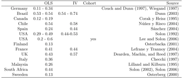
Finally, international evidence on the estimation of the elasticity of income between parents and children show higher mobility in developed countries. However, the relationship with income inequality is not clear. Table 6 in the Appendix shows different estimates of the parameter of interest for selected studies.

3

Data and Descriptive Statistics

For the analysis we combined different birth cohorts of children: children born between 1961 and 1981, and children born in 1966 and 1986. The first group contains sons and daughters in waves 1996 and 2001 that became household heads in the third wave of the panel, year 2006. The second group contains sons and daughters in waves 1996 that became household heads or spouse in 2001 and continued in either of these household categories in the third wave of the panel, year 2006. Therefore, we observe household total income for both groups when they were sons or daughters and when they became household heads or spouse.

The original data contains 9,436 children in total in 1996, from which 3,141 belong to the cohorts defined above. Along with this cohort restriction, the estimation of intergenerational mobility restricts the sample to those children in the cohorts defined for whom we observe household income data when they are children, and those children that became household heads in succeeding waves. Finally, the estimations use a sample size of 1,025 observations.

Francesconi and Nicoletti (2006) estimating intergenerational mobility of occupation for Britain discuss different solutions for sample selection in these kinds of studies when chil-dren/father pairs need to be constructed. They estimate OLS equations considering employment selection and co-residence selection. The former is solved by using Heckman (1979) approach, while the latter considers the selection on the probability of observing children living with their father. The estimations in this article do not use occupational income, but total family income as a measure of wealth, measure that is not bias by employment selection.

Furthermore, by using family income across time as a measure of wealth the estimations in this article do not suffer from co-residence selection bias2_{. However sample selection in terms of}

probability of observing children of cohorts selected as household heads or spouse in succeeding waves may cause a bias.

To correct for this bias we follow Francesconi and Nicoletti (2006) method of propensity score weighting, proposed first by Rubin and Rosenbaum (1984) for correcting the potential bias of this sample selection procedure. In particular, we model the probability of observing children in the cohorts selected as household heads or spouse in succeeding waves. We correct original weights of the panel for this probability and estimate weighted least square equations by OLS to obtain intergenerational elasticities between family income measures.

When pairs of family income in t= 1 andt= 2 are constructed, those observations that are children in 1996 and 2001 and become household heads or spouse in 2006 become two different observations, one being children in 1996 household head or spouse in 2006, and children in 2001 and household head or spouse in 2006. Thus from the 1,025 observations above, the final number of observation increases approximately to 1,700.

Given this sample structure we can observe sons’ and daughters’ household total income in ages that vary between 9 to 35 years old, and their household total income when they become household head or spouse in ages between 20 to 45 years old. In the analysis, we follow Lee and Solon (2006) to consider the effects of observing children income over a range of ages, which may cause a life cycle bias.

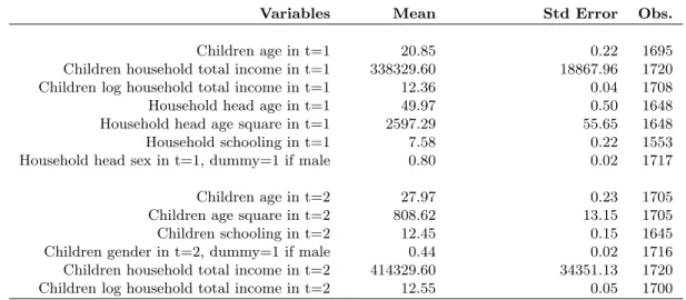
Table 1 shows a descriptive statistical analysis of the data with the variables included in the multivariate analysis. In the period we observe children as sons and daughters (t=1) the mean age is 20.85 years old (within a range of 9 to 35 years for the cohorts chosen). Children’s household mean total income is of $338,329 Chilean pesos (660 USD), household’s head age in t=1 is around 50 years old, have on average 7-8 years of schooling approximately, and 80% of household head in the same period are male. When we observe children as household heads or spouse, their mean age is 28 years old (within a range of 20 to 45 years); they have 12.45 years

2_{In this article we do not use children/father pairs of observations. Pairs of the kindfamily income of children}

of schooling, approximately 44% of them are male, and their household income is on average $414,329 Chilean pesos (813 USD). All incomes expressed here are in real terms, using 1996 as the base year.

Table 1: Descriptive Statistics

Variables Mean Std Error Obs.

Children age in t=1 20.85 0.22 1695 Children household total income in t=1 338329.60 18867.96 1720 Children log household total income in t=1 12.36 0.04 1708 Household head age in t=1 49.97 0.50 1648 Household head age square in t=1 2597.29 55.65 1648 Household schooling in t=1 7.58 0.22 1553 Household head sex in t=1, dummy=1 if male 0.80 0.02 1717 Children age in t=2 27.97 0.23 1705 Children age square in t=2 808.62 13.15 1705 Children schooling in t=2 12.45 0.15 1645 Children gender in t=2, dummy=1 if male 0.44 0.02 1716 Children household total income in t=2 414329.60 34351.13 1720 Children log household total income in t=2 12.55 0.05 1700 Note: All statistics are calculated using adjusted longitudinal weights for sample election

4

Results

Income mobility can be study through different analysis. One of them is the analysis of positional movement using mobility matrices to study mobility between two different categories of the same dimensions (time, generation, geographical, etc.). This way we can study intergenerational mobility by looking at deciles of income where fathers and children are positioned in the exact period when we observe their income.

Table 2 shows a mobility matrix for deciles of income, measured as the total household income. In the rows the table shows the decile of household total income in t = 1, that is when the child has not yet become a household head. In the columns the table shows the deciles of household total income when the child becomes a household head. For instance, the table shows that approximately 29.1% of children whose childhood household was in the first

decile of income, remained in this position when they became household heads. Furthermore, approximately 78% of these children remained in the lowest five deciles of income.

The table shows that mobility is higher in the middle deciles of income. In the highest deciles of income, the table shows that while 39.9% of children whose childhood household was in the tenth decile of income remained in this position when they became household heads, and 85% of them stayed the top five income deciles. This results reflects how mobility decreases as people move into higher levels of income. It seems that between generations income is more mobile in lower deciles. This is consistent with the thesis of Torche (2005) that shows Chile as a country with higher mobility in lower deciles.

Table 2: Mobility matrix of deciles of income

Adult Decile 1 2 3 4 5 6 7 8 9 10 Childhood Decile 1 29.1% 21.4% 10.6% 10.4% 6.5% 7.1% 3.9% 4.6% 4.2% 2.3% 2 19.5% 22.1% 13.8% 11.9% 9.2% 7.5% 5.5% 6.2% 2.5% 1.9% 3 13.0% 16.5% 16.8% 12.3% 12.3% 9.2% 7.8% 5.6% 3.7% 3.0% 4 10.7% 11.8% 13.7% 15.5% 11.1% 11.0% 8.8% 8.1% 5.9% 3.6% 5 7.1% 8.8% 10.5% 13.5% 15.1% 12.0% 9.6% 10.5% 7.9% 5.0% 6 7.4% 8.6% 8.6% 11.8% 12.9% 13.3% 12.9% 10.7% 9.1% 4.7% 7 5.2% 6.0% 7.7% 9.4% 10.3% 13.3% 12.9% 13.0% 13.8% 8.4% 8 4.5% 4.3% 5.6% 8.0% 7.9% 11.7% 13.8% 16.1% 15.4% 12.8% 9 2.7% 3.3% 4.0% 6.0% 7.2% 8.9% 16.1% 14.5% 19.3% 18.1% 10 1.3% 2.4% 2.8% 3.8% 4.8% 6.2% 8.9% 10.9% 19.0% 39.9%

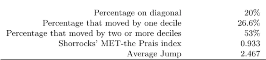
Various measures can be obtained from transition or mobility matrices as shown in Table 3. The first of them shows the percentage of sample members in the diagonal of the mobility matrix. The table shows that 20% of children when they became household heads belong to the same decile of income as their childhood household. The next measure shows that 24% of sample members moved, upwards or downwards, by one decile, while almost 60% of them moved, upwards or downwards, by two or more deciles.

The next two measures are the Shorrocks MET - Prais Index (Shorrocks 1978) and the Aver-age Jump measure. The latter measures the averAver-age jump between deciles of each observation in our sample, while the former is an index that ranges between 0 and 1, where 0 is perfect mobility

of the observations in the sample. The Shorrock’s index shows a value of 0.933, showing a low mobility compared to other developing countries. The average jump shows that children when they become household heads ,move on average 2.4 deciles, upwards or downwards, from their childhood household income decile.

Table 3: Income mobility matrix measures

Percentage on diagonal 20% Percentage that moved by one decile 26.6% Percentage that moved by two or more deciles 53% Shorrocks’ MET-the Prais index 0.933 Average Jump 2.467

Following the descriptive analysis and transition matrices for income mobility, we now present results from the regressions presented in section 2. The complete results of the regression are available in the appendix: Model 1 in Table 7, Model 2 in Table 8, Model 3 in Table 9 and Model 4 in Table 10. . Here we present a summary table for the regressions of income mobility. Section 3 discussed sample selection issues that arose from the sample selection process followed for this research. Original sample weights were adjusted by this selection process. The coefficients shown are estimated using these adjusted longitudinal weights.

Furthermore, we include controls progressively to see the changes in the relevant parameter associated to household in t = 1, though the results reported in this paper show coefficient of regressions with all controls included: age of the child when his or her income as adult is observed, this same age squared, age of the father when childhood household income is observed, this age squared and a dummy for year to control for time specific effects. We also present results for all sample, only sons and only daughters. We recall that the higher the parameter the lower the intergenerational mobility. As we present before, in the international literature this parameter is in general low in Scandinavian countries, is higher in the US and much higher in Brazil, for example3_.

Table 4 shows the childhood/adult elasticities for income estimated from equations in section 2. The first row of table 4 shows an intergenerational income elasticity of 50% for the full sample. The next two columns show this same regression for the sub sample of sons and daughters. As the results show, differences in mobility between sex are noticeable. For instance, while the child/adult elasticity of income is of 60.8% for men, women have an intergenerational income elasticity of 40%. This difference in 20 percentage points suggests that women are more mobile than men when it comes to intergenerational income mobility. That is, women tend to have better outcomes in terms of income mobility than men once they leave their child status in the household. All parameters in Model 1 are statistically significant. The three parameters shown are higher than those of Lee and Solon (2006) for the US4_.

Table 4: Summary table of log-income mobility elasticities: β₁

All Sample Sons Daughters Model 1 0.500*** 0.608*** 0.400*** Model 3 0.479*** 0.562*** 0.404*** Cohort 70 - 80 0.014 0.027 -0.008 Cohort 80 - 90 0.023 0.034 -0.003 Model 4 0.633*** - -Note: *** p≤0.01, ** p≤0.05, * p≤0.1 All Control variables included

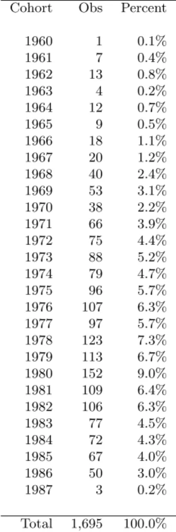
To study time variant effects of income mobility, model 2 estimated the same regressions interacting the log of income with a dummy for each cohort in the data. Table 5 shows the cohort sampling distribution. The cohorts included in this regression are 1966 - 1986, due to low sample sizes in other cohorts. Figure 1 shows how income elasticity varies according to the year of birth. Like Lee and Solon (2006), these results are controled for life cycle bias, by adding age and age square of both child and father in the regression. The figure shows the results for the whole sample, sons and daughters. On average, intergenerational mobility of incccome has decreased on time. The coefficient estimated is higher for younger cohorts. Furthermore,

4_{Lee and Solon (2006) find parameters of 30%. However the cohort analysis showed a wide range of results,}

differences between men and women remain no matter the cohort, though the gender gap has decreased with time. This is mainly due to the fact that women has become less mobile in terms of income relative to men.

Model 3 estimates the cohort analysis, using aggregated cohorts. The sample was separated in three cohorts: born between 19601970, born between 19701980, and born between 1980 -1990. The base group is the oldest cohort. The coefficients shown in Table 4 show that for the whole sample mobility has decreased. In fact, the coefficient is higher for cohort 80 - 90, 50.2% compared to 49.3% in cohort 70 -80, and 47.9% for the base cohort. When this equation is estimated for the sub sample of men, a larger mobility coefficient is obtained, and cohort differences are higher as well. For the sub sample of women the opposite results are obtained: higher mobility and small changes between aggregated cohorts. Finally, when we estimate intergenerational mobility using parental permanent income, we obtained lower mobility than models estimated before, the elasticity using permanent income is 63%. This suggest that using one period of income to estimate mobility underestimates the parameter of mobility.

Table 5: Birth Cohort for child

Cohort Obs Percent 1960 1 0.1% 1961 7 0.4% 1962 13 0.8% 1963 4 0.2% 1964 12 0.7% 1965 9 0.5% 1966 18 1.1% 1967 20 1.2% 1968 40 2.4% 1969 53 3.1% 1970 38 2.2% 1971 66 3.9% 1972 75 4.4% 1973 88 5.2% 1974 79 4.7% 1975 96 5.7% 1976 107 6.3% 1977 97 5.7% 1978 123 7.3% 1979 113 6.7% 1980 152 9.0% 1981 109 6.4% 1982 106 6.3% 1983 77 4.5% 1984 72 4.3% 1985 67 4.0% 1986 50 3.0% 1987 3 0.2% Total 1,695 100.0%

5

Conclusions

This paper investigates intergenerational mobility of income using the longest panel data house-hold survey available in Chile. We followed Lee and Solon (2006) by modeling time-series vari-ation in intergenervari-ational mobility and analyzing cohort’s differences. Our results show a large parameter of correlation between parents’ income and children’s income compared to developed countries which shows low mobility. In addition, cohort’s analysis shows mobility is decreasing as younger cohorts appear to be less mobile than older ones. This results are consistent with the fact that income inequality has remained stable in the last years, as higher mobility is cor-related with lower levels of inequality. The results obtained range from 50% to 63% of income elasticity when the whole sample is used. When the sub samples of men and women are used

for estimations, the results show higher mobility for women than for men.

Bibliography

• Contreras, D., R. Cooper, J. Herman and C. Neilson (2004). Dinamica de la Pobreza y Movilidad Social: Chile 1996-2001, Departamento de Economia, Universidad de Chile, Agosto 2004.

• Francesconi, M. and C. Nicoletti (2006), Intergenerational mobility and sample selection in short panels, Journal of Applied Econometrics, 21, pp.1265-1293.

• Heckman, J. (1979). Sample selection bias as a specification error, Econometrica, 47, 153-61.

• Lee, Chul-In and Gary Solon (2006), Trends in Intergenerational Income Mobility, NBER Working Paper 12007. http://www.nber.org/papers/w12007.

• Nu˜nez, Javier and Cristina Risco (2004) Movilidad Intergeneracional del Ingreso en un Pa´ıs en Desarrollo: El Caso de Chile. Documento de Trabajo No _{210, Departamento de}

Econom´ıa, Universidad de Chile.

• Stephen P. Jenkins and John Micklewright (2007). New Directions in the Analysis of Inequality and Poverty, IZA DP No. 2814, May 2007.

• Rose, D., 2000,Household panel studiesin Rose, D. (ed.), Researching Social and Economic Change: the uses of household panel studies, 3-35, London and New York: Routledge.

• Rosenbaum, Rubin (1984), Reducing bias in observational studies using sub-classification on the propensity score, JASA, 79:516-24.

• Sapelli, C. 2004,Movilidad Social en Chile: Comentarios, Seminario Expansiva.

• Shorrocks, A. F. (1978), Income inequality and income mobility, Journal of Economic Theory 46, 376-393.

• Torche, F. (2005),Unequal but Fluid: Social Mobility in Chile in Comparative Perspective. American Sociological Review, Vol. 70, No. 3 (Jun., 2005), pp. 422-450.

6

Appendix

Table 6: Intergenerational Income elasticities

OLS IV Cohort Source

Germany 0.11 - 0.34 Couch and Dunn (1997), Wiegand (1997) Brazil 0.53 - 0.54 0.54 - 0.74 Dunn (2003)

Canada 0.12 - 0.19 Corak y Heisz (1995)

Chile 0.54 0.58 N´u˜nez y Risco (2004)

Spain 0.24 0.44 S´anchez (2004)

USA 0.29 - 0.49 0.44-0.53 Solon (1992)

USA 0.2 - 0.6 yes Lee and Solon (2006)

Finland 0.13 Osterbacka (2001)

France 0.41 0.44 Lefrane y Trannoy (2004) UK 0.43 0.57 Dearden, Machin, and Reed (1997)

Italy 0.36 Checchi (1997)

Malaysia 0.26 Lilland and Kilburn (1995)

South Africa 0.44 Solon (2002), Solon (2006)

Sweeden 0.13 Osterberg (2000)

T able 7: Mo del 1: OLS of Child Income in t=2. In tergenerational Income elasticities V ariables All Sample Sons Daugh ters Original W eigh ts Adjusted W eigh ts Original W eigh ts Adjusted W eigh ts Original W eigh ts Adjusted W eigh ts Income in t=1 0.505*** 0.500*** 0.590*** 0.608*** 0.426*** 0.400*** (0.035) (0.040) (0.056) (0.065) (0.042) (0.042) Age of child in t=2 0.178*** 0.193*** 0.208** 0.219** 0.191** 0.211** (0.060) (0.066) (0.086) (0.102) (0.077) (0.083) Age of child squared in t=2 -0.003*** -0.003*** -0.003** -0.003** -0.003** -0.004** (0.001) (0.001) (0.001) (0.002) (0.001) (0.001) Age of Household Head in t=1 -0.019 -0.018 -0.082** -0.074* 0.051 0.044 (0.025) (0.027) (0.034) (0.040) (0.041) (0.042) Age of Household Head in t=1 squared 0.000 0.000 0.001** 0.001* -0.000 -0.000 (0.000) (0.000) (0.000) (0.000) (0.000) (0.000) Dumm y =1 for year 2001 -0.179** -0.161** -0.118 -0.130 -0.209** -0.149* (0.077) (0.081) (0.120) (0.128) (0.088) (0.087) W eigh t imputation -0.019 0.299** -0.254* (0.115) (0.145) (0.144) cons 4.210*** 3.979*** 4.223*** 3.574** 3.266** 3.390** (1.035) (1.134) (1.354) (1.641) (1.475) (1.663) Num b er of observ ations 1,604 1,604 700 700 900 900 R2 0.304 0.289 0.363 0.362 0.278 0.263 Note: *** p ≤ 0.01, ** p ≤ 0.05, * p ≤ 0.1

Table 8: Model 2: OLS of Child Income in t=2. Cohort Analysis

Variables All Sample Sons Daughters

Original Weights Adjusted Weights Original Weights Adjusted Weights Original Weights Adjusted Weights Income in t=1 0.418*** 0.421*** 0.467*** 0.477*** 0.337*** 0.316*** (0.065) (0.064) (0.078) (0.076) (0.085) (0.078) Cohort 2 0.013 0.002 0.022 0.014 -0.064** -0.062** (0.032) (0.028) (0.034) (0.030) (0.025) (0.027) Cohort 3 0.043** 0.041** 0.048* 0.040* 0.040 0.041 (0.020) (0.020) (0.025) (0.023) (0.029) (0.029) Cohort 4 0.003 0.004 0.008 0.018 0.004 0.006 (0.020) (0.020) (0.024) (0.025) (0.027) (0.027) Cohort 5 0.037 0.040 0.067* 0.078** -0.007 -0.004 (0.031) (0.032) (0.037) (0.039) (0.034) (0.033) Cohort 6 0.024 0.026 -0.007 0.007 0.049 0.052 (0.031) (0.032) (0.041) (0.041) (0.036) (0.034) Cohort 7 0.023 0.021 0.025 0.026 0.031 0.035 (0.037) (0.037) (0.051) (0.048) (0.043) (0.041) Cohort 8 0.062 0.068 0.063 0.084 0.063 0.071* (0.050) (0.051) (0.064) (0.065) (0.045) (0.042) Cohort 9 0.002 0.005 0.016 0.038 0.008 0.012 (0.044) (0.046) (0.061) (0.063) (0.049) (0.046) Cohort 10 0.034 0.036 0.020 0.039 0.070 0.074 (0.051) (0.053) (0.067) (0.069) (0.056) (0.053) Cohort 11 0.016 0.021 0.016 0.047 0.033 0.036 (0.054) (0.055) (0.071) (0.074) (0.060) (0.056) Cohort 12 0.042 0.048 0.039 0.072 0.067 0.072 (0.058) (0.060) (0.078) (0.081) (0.063) (0.059) Cohort 13 0.052 0.058 0.029 0.069 0.095 0.097 (0.063) (0.066) (0.084) (0.087) (0.068) (0.064) Cohort 14 0.034 0.044 0.039 0.080 0.066 0.077 (0.069) (0.071) (0.096) (0.099) (0.075) (0.070) Cohort 15 0.044 0.051 0.032 0.073 0.084 0.090 (0.071) (0.074) (0.096) (0.099) (0.077) (0.072) Cohort 16 0.045 0.054 0.005 0.048 0.099 0.105 (0.076) (0.079) (0.102) (0.106) (0.082) (0.077) Cohort 17 0.058 0.068 0.060 0.096 0.101 0.111 (0.081) (0.084) (0.108) (0.111) (0.088) (0.082) Cohort 18 0.063 0.068 0.038 0.091 0.126 0.128 (0.086) (0.090) (0.119) (0.124) (0.090) (0.086) Cohort 19 0.058 0.066 0.056 0.109 0.122 0.132 (0.093) (0.096) (0.125) (0.130) (0.101) (0.093) Cohort 20 0.064 0.075 0.085 0.143 0.126 0.137 (0.097) (0.101) (0.131) (0.136) (0.105) (0.097) Cohort 21 0.074 0.079 0.049 0.112 0.159 0.165 (0.101) (0.105) (0.139) (0.145) (0.110) (0.102) Age of child in t=2 0.180* 0.184* 0.146 0.162 0.342*** 0.354*** (0.108) (0.109) (0.142) (0.149) (0.125) (0.122)

Age of child squared in t=2 -0.002 -0.002 -0.002 -0.001 -0.004** -0.004**

(0.002) (0.002) (0.003) (0.003) (0.002) (0.002)

Age of Household Head in t=1 0.008 -0.009 -0.059 -0.053 0.074* 0.061

(0.028) (0.031) (0.037) (0.039) (0.041) (0.042)

Age of Household Head in t=1 squared -0.000 0.000 0.000 0.000 -0.001* -0.001

(0.000) (0.000) (0.000) (0.000) (0.000) (0.000)

Dummy =1 for year 2001 -0.033 -0.002 -0.016 0.123 0.270 0.320

(0.296) (0.310) (0.396) (0.416) (0.328) (0.306) Weight imputation -0.065 0.332 -0.254 (0.133) (0.205) (0.163) Constant 3.638* 3.787* 5.373** 3.910 -0.431 -0.145 (2.191) (2.272) (2.720) (2.947) (2.739) (2.746) Number of observations 1,539 1,539 668 668 867 867 R2 0.336 0.335 0.428 0.441 0.339 0.334 Note: *** p≤0.01, ** p≤0.05, * p≤0.1 19

T able 9: Mo del 3: OLS of Child Income in t=2. Aggregated Cohort Analysis V ariables All Sample Sons Daugh ters Original W eigh ts Adjusted W eigh ts Original W eigh ts Adjusted W eigh ts Original W eigh ts Adjusted W eigh ts Income in t=1 0.488*** 0.479*** 0.552*** 0.562*** 0.431*** 0.404*** (0.035) (0.038) (0.055) (0.057) (0.045) (0.044) Cohort 70 -80 0.010 0.014 0.020 0.027 -0.009 -0.008 (0.015) (0.015) (0.021) (0.022) (0.014) (0.015) Cohort 80 -90 0.017 0.023 0.027 0.034 -0.004 -0.003 (0.020) (0.021) (0.031) (0.032) (0.020) (0.020) Age of child in t=2 0.175** 0.190** 0.181* 0.177 0.241*** 0.255*** (0.073) (0.077) (0.105) (0.115) (0.091) (0.095) Age of child squared in t=2 -0.003** -0.003** -0.002 -0.002 -0.004*** -0.004*** (0.001) (0.001) (0.002) (0.002) (0.002) (0.002) Age of Household Head in t=1 -0.019 -0.018 -0.083** -0.078* 0.049 0.044 (0.026) (0.028) (0.034) (0.040) (0.042) (0.043) Age of Household Head in t=1 squared 0.000 0.000 0.001*** 0.001** -0.000 -0.000 (0.000) (0.000) (0.000) (0.000) (0.000) (0.000) Dumm y =1 for year 2001 -0.126 -0.093 -0.032 -0.012 -0.190* -0.140 (0.103) (0.112) (0.165) (0.178) (0.114) (0.118) W eigh t imputation -0.014 0.361** -0.241 (0.127) (0.155) (0.158) Constan t 4.161*** 3.899*** 4.606*** 4.166** 2.615 2.797 (1.237) (1.319) (1.639) (1.855) (1.633) (1.796) Num b er of observ ations 1,581 1,581 688 688 889 889 8 R2 0.302 0.289 0.362 0.366 0.279 0.264 Note: *** p ≤ 0.01, ** p ≤ 0.05, * p ≤ 0.1

T able 10: Mo del 4: OLS of Child Income in t=2. P ermanen t Income Mobilit y Analysis All Sample Original W eigh ts Adjusted W eigh ts Income in t=1 0.641*** 0.633*** (0.084) (0.104) Age of child in t=2 0.109 0.100 (0.128) (0.123) Age of child squared in t=2 -0.002 -0.002 (0.002) (0.002) Age of Household Head in t=1 0.055 0.049 (0.049) (0.053) Age of Household Head in t=1 squared -0.001 -0.000 (0.000) (0.000) Constan t 1.826 2.202 (1.983) (2.120) Num b er of observ ations 406 406 R2 0.326 0.312 Note: *** p ≤ 0.01, ** p ≤ 0.05, * p ≤ 0.1