ADVANCES IN ARCHAEOLOGICAL GEOPHYSICS: CASE STUDIES FROM HISTORICAL ARCHAEOLOGY
A Dissertation by
TIMOTHY SCOTT DESMET
Submitted to the Office of Graduate and Professional Studies of Texas A&M University
in partial fulfillment of the requirements for the degree of DOCTOR OF PHILOSOPHY
Chair of Committee, D. Bruce Dickson Committee Members, Suzanne L. Eckert
Mark E. Everett Robert R. Warden Michael R. Waters Head of Department, Cynthia Werner
August 2016
Major Subject: Anthropology
ii ABSTRACT
This dissertation presents advanced methods in data processing, statistical analyses, integration, and visualization of archaeogeophysical data to increase the accuracy of archaeological remote sensing interpretation and predictions. Three case studies are presented from an experimental controlled archaeological test site and two nineteenth century historic military archaeology sites at Paint Rock, Texas and Alcatraz Island, California. I demonstrate the ability of the Geonics EM-63 time-domain
electromagnetic-induction metal detector to detect and localize historical metal artifacts at an experimental site and Paint Rock. Moreover, point pattern analysis spatial
autocorrelation statistics were used to detect statistically significant patterns that spatially compacted the amplitude response of the data to improve the localization of artifacts of archaeological significance. The archaeological data was used to determine the spatial and temporal extent of the military camp at Paint Rock and conforms well with the historic record. A virtual ground-truthing was conducted at Alcatraz Island, where the results of a quantitative attribute analysis of ground-penetrating radar data was tested against the georectification of historic maps in order to determine the location, extent, and integrity of historic military features without excavation. These studies increased the information content of archaeogeophysical data via feedback with
statistics, quantitative attributes, controlled experiments, excavation, and georectification modeling in order to increase the predictive capabilities of the methods to answer the most questions with the least amount of costly excavations.
iii DEDICATION
iv
ACKNOWLEDGEMENTS
First, I would like to thank my committee chair, Bruce Dickson, and committee members Suzanne ‘SuS’ Eckert, Mark Everett, Robert Warden, and Michael Waters for their guidance and support during the course of this research. I can never thank you all enough for the many lesson you taught me along the way. The staff in the Anthropology Department, namely Cindy Hurt, Rebekah Luza, and Marco Valadez deserve many thanks for their administrative support, advice, and patience.
I would like to thank Steve Tran for allowing me to construct the controlled test site on his property and Thomas Jennings for helping me ‘seed’ the site with artifacts. I would like to thank the landowners of the Paint Rock site, Fred and Kay Campbell, without them this research would have been impossible. Their valuable input on the area’s history and patience was invaluable. I would also like to thank the Concho Valley Archeological Society (CVAS), especially C.A. Maedgan and Tom Ashmore; and the crew who helped during geophysical data acquisition and subsequent excavations at Paint Rock: Dr. John C. Blong, Calan Clark, Chris Crews, Dr. Gavin Ge, Rose Graham, Justin A. Holcomb, Larkin Kennedy, Josh Knicely, Dr. Thomas A. Jennings, Jameson Meyst, Dr. Dana L. Pertermann, Dr. Michele Raiser, Megan Stewart, and Dawn
Strohmeyer, Scott Willson, Sarah Dickson-Woods. Texas A&M’s Program to Enhance Scholarly and Creative Activities grant and the Department of Anthropology student research grants provided the funding for this fieldwork. Michael Waters and Suzanne Eckert generously provided field equipment and insight.
v
The work at Alcatraz was conducted under Archaeological Resources Protection Act permit PWR-1979-14-CA-02 (GOGA). I would like to thank: the National Park Service; the staff at the park for their assistance and patience while we conducted fieldwork; and Tanya Komas and her students from the Concrete Industry Management field school, California State University Chico, who helped with data acquisition.
I would like to thank my committee and the anonymous reviewers for their helpful comments which greatly improved the quality of the chapters. I am deeply indebted to my friends who helped me along the way – you all know who you are. Finally, I would like to thank my family - especially mom - for their love, encouragement, patience, and support; without them none of this would have been possible. Alesha, thank you for your love, patience, and support.
vi TABLE OF CONTENTS Page ABSTRACT ... ii DEDICATION ... iii ACKNOWLEDGEMENTS ... iv TABLE OF CONTENTS ... vi
LIST OF FIGURES ... viii
LIST OF TABLES ... xiv
CHAPTER I INTRODUCTION ... 1
CHAPTER II ELECTROMAGNETIC INDUCTION IN SUBSURFACE METAL TARGETS: CLUSTER ANALYSIS USING LOCAL POINT-PATTERN SPATIAL STATISTICS ... 8
Introduction ... 8
Methods ... 12
Results ... 28
Discussion ... 34
Conclusions ... 38
CHAPTER III THE BATTLE THAT WAS AND THE BATTLE THAT WASN’T: HISTORICAL AND ARCHAEOLOGICAL INVESTIGATIONS ON THE CONCHO RIVER NEAR PAINT ROCK, TEXAS ... 39
Introduction and Site Setting ... 42
Historical Background ... 45
Archaeological Background ... 54
Methods ... 56
Results and Discussion ... 63
vii
CHAPTER IV FATE OF THE HISTORIC FORTIFICATIONS AT ALCATRAZ ISLAND BASED ON VIRTUAL GROUND TRUTHING OF GROUND-PENETRATING RADAR INTERPRETATIONS FROM
THE RECREATION YARD ... 73
Introduction ... 73
19th Century Historical Context ... 77
Recreation Yard ... 81
Georectification Modeling ... 84
GPR and Laser-scan Acquisition and Processing Methods ... 88
GPR Interpretation and Discussion ... 98
Conclusions and Future Research ... 108
CHAPTER V CONCLUSIONS ... 110
Experimental Tests and Historic Models ... 112
Quantitative Attribute Analysis and Statistics ... 113
Reflexive Ground-Truthing: Real and Virtual ... 114
viii
LIST OF FIGURES
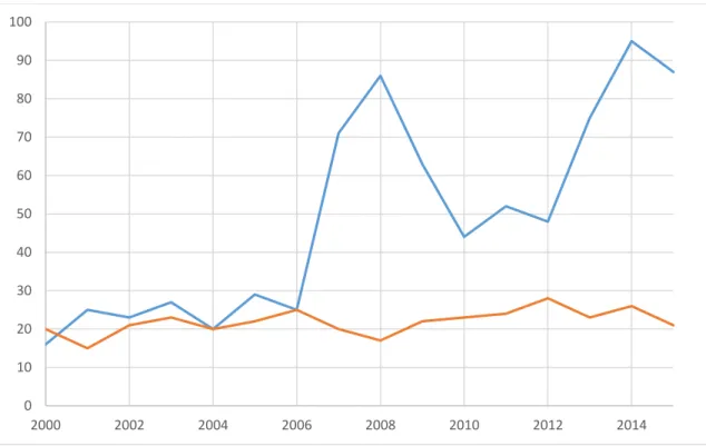
Page Figure 1 Archaeological geophysics papers in the flagship journal of
archaeogeophysics Archaeological Prospection (in red, n=150) and from numerous journals in a Science Direct search for “archaeology geophysics” (in blue, n=768) between 2000-2015. Note the drop in papers during the Great Recession, which began in December 2007. Generally, however, the trend (r2=0.7) of more archaeolpogical
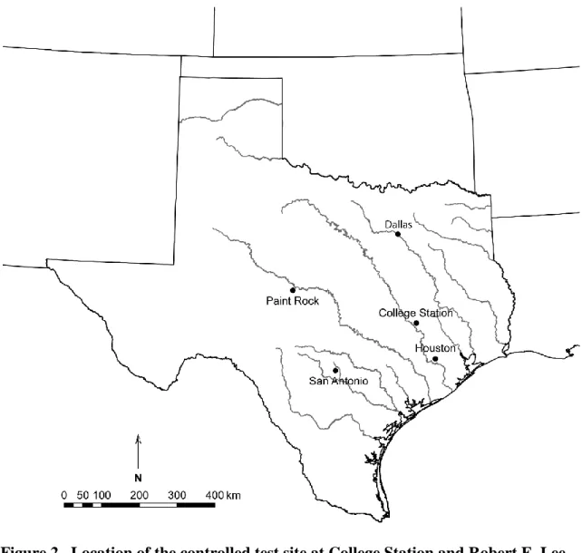
geophysics research should continue in the decades to come ... 2 Figure 2 Location of the controlled test site at College Station and Robert E.
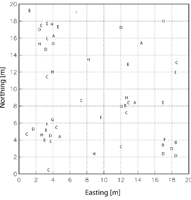
Lee Campsite archaeological site at Paint Rock. The major rivers of Texas and some large cities are included to aid orientation ... 13 Figure 3 Distribution of seeded artifacts, symbol-coded by type, at the Tran
test site: (a) bolt, (b) washer, (c) cylinder, (d) bottle cap, (e) coke can, (f) bullet, (g) license plate, (h) rebar, (i) musket ball. Plot
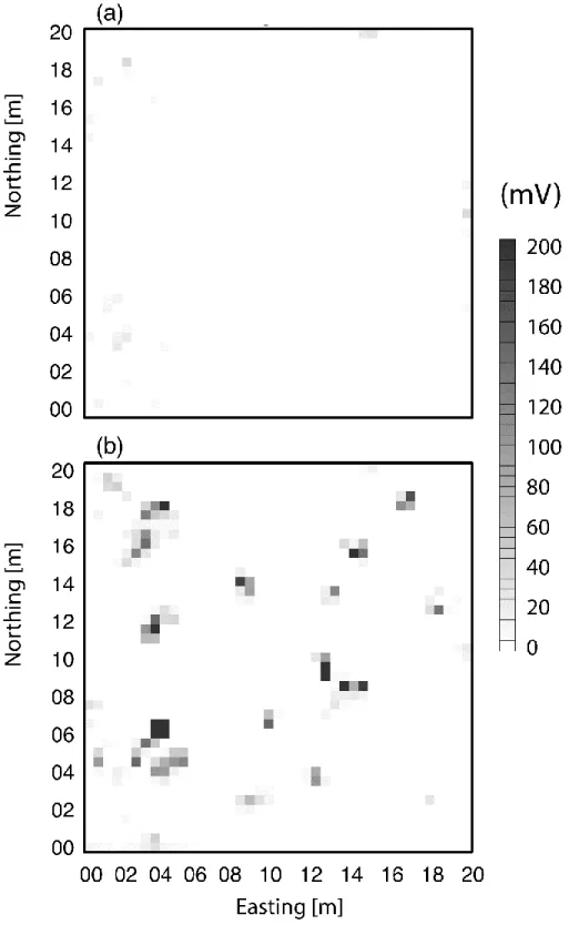
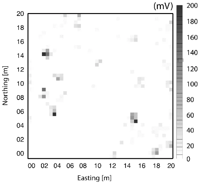
dimensions in m ... 16 Figure 4 EM-63 channel-1 data acquired at the Tran test site: (a) before;
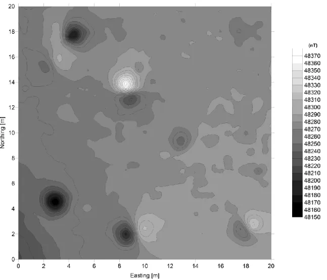
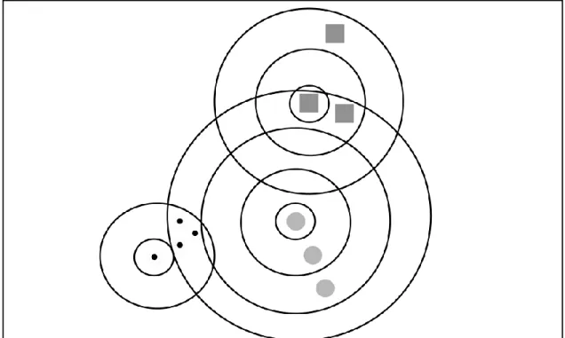
and (b) after seeding with artifacts ... 17 Figure 5 G-858 magnetometer total field data set from Tran site ... 18 Figure 6 EM-63 channel-1 data acquired at the Robert E. Lee campsite ... 20 Figure 7 Illustration of spatial clustering. Circles with integer radius are
drawn about three specified events: black circle, grey circle, and grey square. There is clustering around the black circle event at radii 1<d<2. The same clustering is recorded at 3<d<4 around the grey circle event. The grey circle event, like the grey square event,
shows no clustering at small radii 1<d<3 ... 23 Figure 8 Gi*(d) statistic for stratified datasets at Tran Site: (a) ‘clustered’
license plate at (3.5, 6.5); (b) ‘clutter’ rebar at (3.5, 11.5); (c)
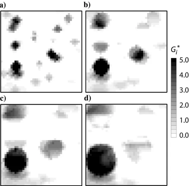
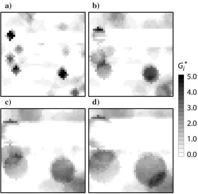
comparison of (a) and (b) for the entire dataset ... 31 Figure 9 Gi*(d) significance maps, Tran Site: (a) d=1.0; (b) 2.0; (c) 3.0;
and (d) 4.0 m ... 32 Figure 10 Gi*(d) significance maps, Lee campsite: (a) d=1.0; (b) 2.0; (c) 3.0;
ix
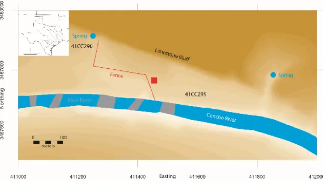
Figure 11 Map of Paint Rock sites 41CC290 and 41CC295. Fords are in grey. Springs and Concho River are in blue. Fence line and 20 x 20 m geophysical survey block in red. Contour interval 1 m. The pictographs were painted, penciled, and incised on the steep limestone bluff, which has many shallow rock shelters. Grid in
UTM northing and eastings, 1.0 x 0.5 km ... 43 Figure 12 Texas forts built during the Statehood Period (1845-1861) and
their dates of use prior to the Civil War in parentheses. The blue stars are forts founded between 1845 and 1850, while the red dots are forts constructed after 1850. After 1850 the civilian settler frontier and military fort systems spread to the west. Paint Rock, Fort Mason, and Fort Chadbourne are in larger font in west-central Texas. Major rivers and modern cities are included to aid
orientation ... 51 Figure 13 (a) Historic graffiti at Paint Rock. ‘HOBAN 1856’ is faded, but
was painted over probable Comanche and/or Apache pictographs. Scale is 10 x 2 cm. (b) Spanish Mission with incised graffiti name ‘L.C. Gibson Aug 1880.’ Perhaps nowhere at the site more clearly demonstrates the shift from a Native American site and assemblage to an Anglo dominated one. The Native American pictographs are
literally written over, but not completely erased ... 52 Figure 14 Graniteware sherds with Anthony Shaw’s maker’s mark, which
dates to between 1850-1882. These are possibly from then Col.
Robert E. Lee’s service ... 55 Figure 15 Geonics EM-63 time-domain electromagnetic-induction
channel-1 data at 41CC295, in mV. Grid oriented north in m. For grid location at Paint Rock see Figure 11. Location of the thirty-three 1 x 1 m excavation units are overlain on the contour
map ... 64 Figure 16 Weighted K-function of Geonics EM-63 time-domain
electromagnetic-induction channel-1 response at 41CC295 over (a) a threshold stratified dataset of response > 25 mV where n=58 and (b) over the entire dataset where n=1,681. The observed L(d) is greater than the maximum L(d) because the data are
significantly clustered at all distance scales in (b) while significant
x
Figure 17 Gi*(d) significance map at 41CC295: (a) d = 1.0; (b) 2.0; (c) 3.0; and (d) 4.0 m. Same 20 x 20 m grid as Figure 15, oriented north. The α is on the left side of the scale bar to illustrate this relationship between the Gi*(d) statistic values, p-values, and statistical
confidence. Since the Gi*(d) values of 3.835, 4.009, 4.378, and 4.836 for n=1681 are equivalent to statistical p-values of α=0.1, 0.05, 0.01, and 0.001 respectively, the odds of a Type I error, or
false positive, are 10, 5, 1, and 0.1% ... 68 Figure 18 Select diagnostic and representative artifacts from Paint Rock sites
41CC290 and 41CC295: (a) pistol frame and barrel, (b) picket pin, (c) three-tine forks, (d) .69 caliber musket balls, (e) toe-clip rim horseshoe, (f) decorative saddle skirt ornament, (g) Eagle and Stars powder flask, (h) saddle rings, (i) 3 Merry widows condom case, (j) flattened federal eagle buttons (k) federal eagle great coat
buttons, (l) .58 caliber Minié balls, (m) spur ... 70 Figure 19 Map of San Francisco Bay showing Alcatraz island and Fort Point.
Red on the state of California inset map is the location of San
Francisco county ... 75 Figure 20 Illustration of common military earthwork architectural features
deployed at Alcatraz [credit: Golden Gate NRA, Fort Point/GG
Bridge CLR, with alterations by John Martini] ... 78 Figure 21 (a) Third System masonry [credit: National Archives] and (b) later
earthwork fortifications on Alcatraz Island facing the city of San Francisco [credit: Golden Gate NRA, Park Archives, Interpretive Negative Collection, GOGA-2316]. Note the caponier, the brick building in (a), was later reduced to half its height and then buried (its location is marked by the red arrow) during the earthwork fortification period of the island’s history. Also marked in red
squares are ventilation ducts above the masonry magazines ... 80 Figure 22 (a) The construction of the military prison, with stockade in the
foreground [credit: National Archives]; (b) the stockade during the military prison era [credit: Golden Gate NRA, Park Archives, William Elliot Alcatraz Photographs, GOGA 40058]; (c) The recreation yard during the federal penitentiary era [credit: Golden Gate NRA, Park Archives, Betty Walker Collection, GOGA]; (d) the recreation yard today as part of the national park. Note that during the military prison era the recreation yard had a grass surface, but during the federal penitentiary era it was converted to concrete. Note the dark stains of the original soil versus the lighter colored
xi
soil fill placed during the construction highlighted in red in (a) ... 83 Figure 23 Historic map of Alcatraz island c.1894 with Traverses I, J, and K
and batteries 6 and 7 noted in red ... 84 Figure 24 (left) Georectified model over the recreation yard based upon the
1894 map where Traverses I, J, and K can be seen from north to south; and (right) georectified sketch map of historic traverses I, J and K and batteries 6 and 7 based on 1892 ordnance survey map, overlain in by the approximate outline of the recreation yard walls (by Martini). The georectification on the left highlights the external architecture while the internal architecture of the masonry
magazines and communication tunnels is shown on the right ... 86 Figure 25 Exploded view (from top to bottom) of the lidar scan, a GPR data
cube, the 3D SketchUp model, and the geo-rectified map of the recreation yard in 2D perspective. Green arrows point to
communication tunnels between traverses. Traverses I, J, and K
and batteries 6 and 7 are marked in yellow ... 87 Figure 26 GPR sections showing the radar signature of buried traverse J (the
prominent hyperbolic return in the middle of the sections, near the bottom at two frequencies: (top) 200 and (middle) 500 MHz data prior to migration; and (bottom) migrated close up of 12-19 m along middle 500 MHz profile with no exaggeration of vertical scale. The 200 MHz profile lacks the resolution of the 500 MHz profile due to the range-to-resolution trade-off. Architectural features associated with each of the traverses can be seen in profile from right to left I, J, and K. The thin red stratigraphic layer in the top left is the interface between the concrete added in 1936 and imported fill materials from the 1907 construction of the prison. The area in the top right is the baseball diamond, which was never overlain with concrete. The strata between the concrete and bottom of the imported fill material is demarcated with a yellow line and can also be seen in Figure 22a. The fill material below this is likely from the original traverses and slopes of the batteries. The red box in the center is the original earthwork traverse and the line below marks the reflection of the vaulted brick and concrete architecture, and dates to 1868-1907. The bottom profile demonstrates the difficulty of presenting long profiles with great vertical exaggeration. These look almost like point source reflectors in the top and middle profiles when exaggerated, but are probably analogous to – anthropogenically transported - onlap backdune deposits. Note the approximately 30
xii
Figure 27 The efficacy of 0.09 m/ns migration: (top) profile before migration, note the two hyperbolic reflections at approximately 1.0 m depth; (second from top) data migrated at 0.13 m/ns, which is too fast, hyperbolae are not collapsed but over migrated to form smiley faces and also inaccurate depth estimates; (second from bottom) data migrated at 0.05 m/ns, which is too slow, hyperbolae are not properly collapsed by migration, and also at inaccurate shallow depths; and (bottom) data migrated at 0.09
m/ns, just right, and they are properly collapsed ... 92
Figure 28 GPR energy and instantaneous amplitude depth slices. Red lines highlight architectural features seen in the georectifications in Figure 24 and dark (black) is high and light (white) is low amplitude. The yellow line in the instantaneous amplitude depth slice between 1.2-1.5 m is the profile seen in Figure 26. The linear white features in the north are uncollected areas due to the baseball diamond fence and the green in instantaneous amplitude depth slice 0-0.3 m are the baseball diamond and rebar reinforced shuffle boards, the last addition to the recreation yard and the only rebar in the
recreation yard floor ... 96 Figure 29 TLS and GPR 500 MHz instantaneous amplitude depth slices
from the recreation yard, at: (a-b) 0.5-1.0 m; (c-d) 1.0-1.5 m depths. (a) and (d) show the common aerial view, while (b) and (c) show a 3D perspective view ... 98 Figure 30 (a) Historical photo, taken during demolition of earthen
fortifications c. 1910 on site of Battery 2, showing the ventilation ducts (two white cylindrical structures in red boxes) located at the top of the concrete magazine and vaulted brick and concrete architecture. National Archives, Record Group 92, OQMG, General Correspondence 1890-1914, Item #223810; and (b) photo showing common earthwork communication tunnel from the later
1800s with ventilation ducts and tunnel in red ... 101 Figure 31 Improved georectification based upon GPR data at: (top) 0.5-1.0
and (bottom) 1.0-1.5 m. Yellow box on top is the morgue and yellow box on the right hand side is the remnant of Traverse K’s magazine. Note the ventilation ducts align with the internal
architecture at bottom ... 103 Figure 32 The 3D SketchUp model in its modern context as defined by GPR
data, within context of TLS data, showing a GPR instantaneous amplitude profile with zoomed in portions of the profile highlighting
xiii
the architecture of traverse J and parapet wall of battery 7 and
xiv
LIST OF TABLES
Page Table 1 Number of neighbors calculated by the local Gi*(d)statistic ... 26 Table 2 Significance Values of the local Gi*(d) statistic at the 90, 95, 99,
and 99.9th percentiles for various sample sizes (α=0.10, 0.05, 0.01,
and 0.001 respectively) ... 27 Table 3 Chi-squared test for the local Gi*(d) statistical predictions based
upon excavations at Paint Rock, where threshold is Gi*(d) values
>3.835 (n=26). Χ2 = 9.9005, df = 1, p-value = 0.001652 ... 37 Table 4 Chi-squared test for the predictions based upon traditional measures,
herein defined as one standard deviation above the mean (channel-1 responses >21 mV, n=51), based upon excavations at Paint Rock.
Χ2 = 3.6397, df = 1, p-value = 0.05642 ... 37 Table 5 Chi-squared test for the local Gi*(d) statistic based upon excavations
at Paint Rock, where threshold is Gi* >3.0 (n=44) at d=1 m;
χ2=16.05, df=1, p-value significant at α <0.0001 ... 67 Table 6 Select representative and diagnostic artifact assemblage at Paint
1 CHAPTER I INTRODUCTION
Since the 1990s a series of advances in computing and electrical engineering have led to the production of less costly, less bulky, more sensitive and efficient
geophysical data acquisition instruments and access to greater data processing power via smaller and faster personal computers (Conyers 2013; Gaffney2008; Linford 2006). By the twenty-first century (Figure 1) near surface geophysical techniques had gained widespread use and acceptance as yet another important methodological implement in the archaeologists toolkit (Agapiou and Lysandrou 2015). In a recent review of
geophysical techniques in archaeology, Gaffney (2008) predicted that advancements in data analyses were likely to be significant research subjects in the next decade of archaeological geophysics (or archaeogeophysics). The following research illustrates various methods to increase the accuracy of archaeological remote sensing interpretation and prediction via advanced processing, integration, visualization, and statistical
2
Figure 1. Archaeological geophysics papers in the flagship journal of
archaeogeophysics Archaeological Prospection (in red, n=350) and from numerous journals in a Science Direct search for “archaeology geophysics” (in blue, n=768) between 2000-2015. Note, the drop in papers during the Great Recession, which began in December 2007. Generally, however, the trend (r2=0.7) of more
archaeological geophysics research should continue in the decades to come.
Advances in the integration of archaeogeophysics data generally takes two forms. In the first multiple geophysical methods are quantitatively or qualitatively integrated in an attempt to better interpret features of interest (Ernenwein 2008, 2099; Kvamme 2006a, 2007). In the second multiple data sets are presented in a single visual image to aid interpretation. This research expands upon the visualization of multiple geophysical data sets via the integration of ground-penetrating radar (GPR) and lidar data with 2D
0 10 20 30 40 50 60 70 80 90 100 2000 2002 2004 2006 2008 2010 2012 2014
3
and 3D historical models. Presenting the GPR past in the context of the 3D lidar point cloud present increases the interpretability of GPR data (Goodman and Piro 2013).
Advanced processing of GPR data via attribute analysis began in the geophysics research community in the 1990s as an offshoot of seismic attribute analysis processing methods. These advances are only possible due to the ability to digitally store data for subsequent processing with smaller, faster, less expensive personal computers (Conyers 2013). Attribute analysis methods quantify the GPR data signal to extract more
information from the data, which relates to subsurface physical processes such as dielectric permitivity contrasts, permeability, stratigraphic interfaces and thickness (Zhao 2013a, 2013b). By the early 2010s the use of GPR attribute analysis methods spread to the archaeology research community (Böniger and Tronicke 2010a, b;
Creasman et al. 2010; Khwanmuang and Udphuay 2012; Udphuay et al. 2014; Urban et al. 2014; Zhao et al. 2012, 2013a, 2013b, 2015a, 2015b). This research adds to a
growing body of literature that seeks to increase the accuracy of archaeological interpretation via advanced processing, which better visualize and quantify patterns related to subsurface physical properties.
The visual presentation of integrated data holds great potential for community outreach and the public dissemination of complex data in both an appealing and accurate way. Tax based funding often supports archaeogeophysical research; however, public stakeholder do not always get to see the results of their investment. Rather, the results are often disseminated by scientist to scientists at professional conferences, in technical journals, and buried in the gray literature of compliance permit reports – all of which are
4
generally unintelligible and non-accessible to the public at large. Moreover, presenting the results and interpretation of geophysical research to the public is particularly difficult because GPR profiles look like a Rorschach test to those untrained in geology and geophysics. Therefore, the role of advanced data processing and visualization to aid interpretation for public education and outreach efforts cannot be under stressed; here the challenge is to explain the layout of archaeological artifacts and features with interpretive illustrations and geophysical data.
Statistical analyses of single or multiple methods archaeogeophysical surveys seeks to quantify significant patterns in data sets to reduce errors cause by unsystematic qualitative anomaly hunting. Interpretational errors are costly in terms of time and labor and therefore money, but also in terms of destructive excavations. Statistical analyses of archaeogeophysical data can reduce the time, labor, and monetary costs of research. Most importantly, however, increasing the confidence of interpretation and predictive capabilities of archaegeophysical data via statistical analyses holds the greatest potential for the advancement of preservation archaeology and the stewardship of the
archaeological record.
Despite the recent advances in archaeological geophysics (Gaffney 2008; Linford 2006), great skepticism of the methods abounds (Jordan 2009), particularly in the United States where the application of geophysics in archaeology lags behind Europe (Johnson 2006; Thompson 2015). Remote sensing is often assumed to be highly quantitative because the methods are based in the ‘hard’ science; however, the interpretation of these data is often no more than qualitative X marks the spot ‘anomaly’ hunting (Conyers 2013;
5
Gaffney 2008; Jordan 2009), a situation that can lead to erroneous interpretations and a lack of confidence in the discipline. This research proposes to increase the reliability of archaeological geophysics interpretations in three key ways: (1) through the use of control experimental sites and georectification of historic maps at historical archaeology sites to create middle-range analogies to test cultural and natural processes; via (2) the application of rigorous quantitative analysis of geophysical data through geostatistics and various mathematical data filtering methods (attribute analysis); and via (3) ground-truthing excavations, which provides feedback to iteratively improve predictions.
These goals were accomplished by examining three case study sites: (1) the experimental controlled historical archeology test site in College Station, Texas; (2) the Paint Rock, Texas, battlefield and historical military camp sites (41CC1, 290, 295); and (3) the historic fortifications on Alcatraz Island, California.
In Chapter II results are presented from the Tran experimental control archaeology site where I conducted time-domain electromagnetic induction (EMI) surveys with the Geonics EM-63 before and after emplacing replica historical artifacts. The spatial structure of the EMI data was assessed with global and local point-pattern analysis (PPA) autocorrelation statistics, namely the global K-function and local Getis-Ord Gi*(d) statistics. Results suggest that the Geonics EM-63 can be used to locate historical metal artifacts and that the PPA statistics can determine significant clustering of artifacts while also compacting the spatial footprint of the EMI amplitude response.
I then tested the real world application of EMI and PPA at the Paint Rock historical archaeological battlefield and camp site discussed in Chapter III. In order to
6
better understand the landscape scale turnover in artifact assemblages during the mid-nineteenth century at historical military archaeology sites the theoretical perspective of ‘eventful sociology’ (Sewell 2005:100) was employed. Eventful sociology was
operationalized for archaeology by Beck and colleagues (2007) and utilizes both structuration (Giddens 1984; Sewell 1992) and practice/agency theory (Bourdieu 1977, 1984). Results suggest that the military presence at the site dates to the 1850s to 1870s and extends between the springs and first terrace on the north side of the Concho River. The results of the EMI and PPA statistics are applicable in a real world archaeological context.
In Chapter IV, I use geographical information systems (GIS) software to georectify historic maps to create testable hypotheses as to the possible location of historic military fortifications on Alcatraz Island, California. GPR data were used to physically test the georectification model, to virtually ground-truth (VGT) the site, without excavation. A quantitative attribute analysis of the GPR data was used to better determine the true location, extent, and integrity of subsurface archaeological remains from the late 1800s. Results suggest that the advanced processing techniques of migration and attribute analysis are able to detect the location, extent, and integrity of subsurface archaeological features that date to the military earthwork fortification period on the island.
As physical anomalies may not be represented materially, archaeological excavation is the only way to definitively asses and validate the interpretations of near-surface applied geophysics data (Hargrave 2006); however, excavations are inherently
7
destructive and permanently remove buried artifacts from their primary context. It is sometimes said that “archaeology is the only branch of anthropology where we kill our informants in the process of studying them” (Flannery 1982:275). Excavation is not only invasive and destructive, but it is also time consuming and labor intensive, and therefore expensive (Johnson and Haley 2006). Moreover, at many cultural heritage sites excavations may not be desirable or possible. An ideal archaeological investigation of the subsurface based mainly upon interpretations of remote sensing data would be accurate enough to require minimal excavations, answering the most anthropological research questions with limited excavations, thereby preserving as much of the valuable non-renewable in situ cultural resources as possible for future generations (Doelle and Huntley 2012). The potential of geophysical methods for preservation archaeology is the foundation for the future of the ethic of stewardship of the archaeological record, for we cannot protect our cultural resources if we do not know what they are and where they are located.
8 CHAPTER II
ELECTROMAGNETIC INDUCTION IN SUBSURFACE METAL TARGETS: CLUSTER ANALYSIS USING LOCAL POINT-PATTERN SPATIAL STATISTICS*
Introduction
Clustering of subsurface metal targets is important in near-surface geophysical application areas such as unexploded ordnance (UXO) remediation, mineral exploration, environmental or geotechnical site assessment, and historical or industrial
archaeology. The spatial distribution of metallic targets can reveal information about the natural or anthropogenic spatiotemporal processes which led to the emplacement of objects that are now of historical, cultural, environmental, economic, geotechnical, or archaeological significance. Electromagnetic geophysical measurements offer a powerful noninvasive probe of subsurface metal distribution. The data, carefully analyzed, can be used to test and discriminate hypotheses about the underlying site formation processes. Spatial cluster analysis is relevant to archaeological reconstructions or site assessments since artifacts that are associated with a past event such as a battle, or past industrial use such as a foundry or railyard, tend to be found in close proximity (Schwarz and Mount 2006). At brownfields sites scheduled for reclamation or re- ________________________
* Reprinted with permission from “Electromagnetic induction in subsurface metal targets: Cluster analysis using local point-pattern spatial statistics” by T.S. de Smet, M.E. Everett, C.J. Pierce, D.L. Pertermann, and D.B. Dickson, 2012, Geophysics, Volume 77, Number 4, pp. WB161-WB169, Copyright 2012 Society of Exploration Geophysics.
9
development, due to past land-use patterns there often develops clustering of targets of interest, such as underground pipes, drums, or storage tanks or the buried remnants of reinforced concrete foundations.
A wide variety of methods are available to discern patterns in spatial data (Perry et al. 2002), including self-organizing maps (Benavides et al. 2009), various clustering algorithms (Paasche and Eberle 2009, 2011), and numerous global and local point pattern analysis (PPA) techniques (Getis and Ord 1996). Global PPA of geophysical responses discriminated UXO from clutter at a practice bombing range in which the UXO was deposited according to known aircraft flight patterns while the clutter was randomly distributed (MacDonald and Small 2009).
Paasche and Eberle (2009, 2011) in the context of mineral exploration have recently discussed and utilized numerous clustering algorithms like k-means, fuzzy c-means, and the Gustafson-Kessel method. One major drawback of these techniques is that the number of clusters must be chosen prior to analysis, regardless of whether clustering is actually present in the data set. As such the usefulness of these clusters must be verified against external criteria. With local statistical measures of spatial
autocorrelation, as used in this paper, no a priori assumptions are made about the number of clusters.
The preferred geophysical technique for detecting subsurface metal items is transient electromagnetic induction (EMI). The EMI data analyzed in this paper were collected with a Geonics EM-63 metal detector (www.geonics.com). The EM-63 records
10
a time-decaying voltage at the receiver (RX) coil after a sudden switch-off in the magnetic field generated by the transmitter (TX) coil. The RX voltage decay is due to the dissipation of eddy currents that are induced in the host geology along with any subsurface metal targets of sufficient inductance (Everett 2005) that are buried within several m of the surface. The RX voltage is digitized at 26 time gates, or channels, that are logarithmically spaced from t0=180 s to t1=25 ms after TX switch-off.
The EM-63 normally detects targets whose characteristic size a, magnetic permeability μ, and electrical conductivity σ are such that the eddy-current diffusion time satisfies τ>t0 where τ~μσa2 (Pasion 2007; Benavides et al. 2009). The shape of the RX voltage waveform is indicative of target characteristics. The amplitude of the early-time RX voltage response, for instance, reads higher than background geological noise levels for all detectable metal artifacts whether small or large, shallow or deeply-buried. The late-time RX voltage response remains high, however, only for the larger objects for which τ>>t0. An important diagnostic of such large objects, therefore, is the lengthy time that is required for the induced eddy currents, and hence the RX voltage, to decay to the instrument noise level. As the amplitude response is measured at 26 time gates, the initial response and shape of the decay curve could be used to roughly classify the depth, orientation, and size of specific anomalies.
In this paper we consider two features of the EM63 response: (a) the magnitude of the early-time RX voltage response [mV] (hereinafter called the channel-1 response); and (b) the time gate at which the RX voltage decays to the instrument noise level (hereinafter called the decay time). The channel-1 response reads high for all detectable
11
metal targets while a lengthy decay time can be used to preferentially select the larger ones.
Local PPA is used herein to detect and locate target clustering. The precise identification and location of target clusters helps stakeholders to better comprehend site formation processes and to develop an efficient excavation strategy. We weight points according to their EM63 channel-1 response and decay time. The location of the most interesting clusters is identified using the local Gi* statistic (Getis and Ord 1992, 1996; Ord and Getis 1995).
The plan of the paper is as follows. First, we suggest an EM63 acquisition technique that ensures a high quality data set. We then review elements of the point pattern statistical methodology. EM-63 data are presented from a controlled test site seeded with a known spatial distribution of common metal artifacts, and from a historical archaeological site, the Robert E. Lee camp at Paint Rock, Texas. The latter site, centrally located between Fort Mason and Fort Chadbourne, c.1851-1874 was utilized by the US Second Cavalry and many other troops, most notably then Colonel Robert E. Lee in 1856 (Freeman 1934). At both sites we show how point pattern spatial statistics can be used to describe and locate the clustering of subsurface metal targets identified by EM-63 responses. Excavation results from Paint Rock are analyzed. The results demonstrate the utility of the approach for archaeological site formation
12 Methods
EMI data were acquired with the Geonics EM-63 at a controlled test site and an active archaeological site in Texas (Figure 2). The Tran experimental site is located in College Station, Brazos County, about 7 km east of Texas A&M University (TAMU). The Robert E. Lee campsite (U.S. registered archaeological site no. 41CC295) is located in the town of Paint Rock in Concho County on a terrace of the Concho River near a series of natural fords. Both sites are flat grassy pastures characterized by floodplain deposits of clays, silts, and clayey sands.
13
Figure 2. Location of the controlled test site at College Station and Robert E. Lee Campsite archaeological site at Paint Rock. The major rivers of Texas and some large cities are included to aid orientation.
The Geonics EM-63 is a transient controlled-source electromagnetic induction instrument arrayed in the central-loop configuration. The transmitted current, which generates a primary magnetic field, is suddenly switched off, inducing a secondary magnetic field which decays slowly in subsurface ferrous and non-ferrous metal targets. After the primary field is switched off, the secondary magnetic field is recorded at 26
14
logarithmically-spaced time gates. The eddy currents induced in metal objects of different size, shape, strike, and orientation decay at characteristic rates, thus enabling a rudimentary target classification prior to excavation. The transient EM response
amplitude, measured in mV, and its time rate of decay, measured in mV/s, can generally be used to predict the size and depth of subsurface anomalies. For instance, a small channel-1 response exhibiting a slow decay time typically indicates a large metal object at depth, whereas a higher channel-1 response accompanied by a brief decay time suggests a shallower burial.
Data Acquisition
An improved data acquisition protocol was developed to provide accurate sensor navigation, as required by the spatial statistics methods used in this study. Slight
irregularities in the terrain causes loss of control of the EM-63 when it is deployed in the conventional cart-mounted configuration. The EM-63 was mounted on a sled and pulled along the survey lines. Data on an accurate rectilinear grid are straightforward to acquire in this fashion, with consistent positional accuracy to within a few cm, using manual data triggering. Data acquisition times using the cart and sled systems are similar.
15 Tran Experimental Site
The improved acquisition protocol was used to evaluate the performance of the EM-63 for spatial cluster analysis at a controlled test site seeded with metal artifacts. For this purpose, a clean site on private land was selected. The landowner Mr. S. Tran stated that the site is used for agricultural purposes and that subsurface metal objects are not expected. The site was seeded by a number of common metal items in the spatial pattern shown in Figure 3. In order to test the ability of the statistics to discriminate between clustering and random spatial patterning, we purposely buried 32 of these items in four clusters (these are called “artifacts”) and another 18 at randomly chosen locations (these are called “clutter”). A background EM-63 data set was acquired prior to the seeding (Figure 4a), in which minor and widely scattered EM-63 signals are observed. The line spacing and the station spacing are both 0.5 m for the 20 x 20 m survey area, for a total of 1681 data points. A second EM-63 data set was then acquired after seeding. The resulting EM63 channel-1 response of the seeded site (Figure 4b) clearly reflects the spatial distribution of the shallow buried items.
A third data set was acquired at the site using the Geometrics G-858 cesium-vapor magnetometer (www.geometrics.com) in order to compare the capabilities of EMI and magnetometry for target cluster analysis (Figure 5). Magnetometry is widely used in archaeological prospection (Conyers and Leckebusch 2010; Kvamme 2006b; Perttula et al. 2008) and UXO mapping and detection (Beard et al. 2008; Doll et al. 2008), sometimes in conjunction with EMI (Beard et al. 2008; Pétronille et al. 2010). The
G-16
858 magnetometer is a passive device that measures the intensity of the sum of the background geomagnetic field and the much smaller magnetic field due to any nearby ferrous objects.
Figure 3. Distribution of seeded artifacts, symbol-coded by type, at the Tran test site: (a) bolt, (b) washer, (c) cylinder, (d) bottle cap, (e) coke can, (f) bullet, (g) license plate, (h) rebar, (i) musket ball. Plot dimensions in m.
17
Figure 4. EM-63 channel-1 data acquired at the Tran test site: (a) before; and (b) after seeding with artifacts.
18
Figure 5. G-858 magnetometer total field data set from the Tran site.
The G-858 and EM-63 instruments have complementary capabilities. The EM-63 responds to all conductive metal objects, whereas the G-858 detects only ferrous targets. A G-858 data set does indicate, however, the background spatial variation of magnetic soils and sediments. The G-858 yields a spatially distributed pattern of dipole
anomalies, rather than a discrete point set, since the magnetic signature of a buried target is dipolar and often merges with neighboring signatures. Spatial filtering by methods such as reduction-to-pole, analytic signal, or regional subtraction are required to better
19
isolate the magnetic signatures, whereas virtually no processing is necessary with EM data. For this reason, the G-858 data set is not as amenable as the EM-63 data set to target cluster analysis using point-pattern spatial statistics. A qualitative visual inspection of Figure’s 4 and 5 demonstrates that EM-63 anomalies are more compact than their G-858 counterparts - note especially the isolated rebar at coordinates (2, 9) and (8, 13).
Archaeological Case Study at Paint Rock
An EM-63 data set was acquired at the Robert E. Lee campsite (Figure 6) over a 20 x 20 m grid with 0.5 m line and station spacing, for a total of 1681 measurements. The site was previously scanned with hand held metal detectors by the local avocational archaeological society (Ashmore, 2010) to identify subareas most likely to yield historic metal artifacts. This is standard archaeological practice (Bevan 2006; Connor and Scott 1998). The EM-63 data sets were analyzed using point pattern statistical methods, which are described in the next section of this paper. The PPA program (Aldstadt et al. 2002) is a statistical toolbox designed for spatial analysis applications, including cluster analysis.
20
Figure 6. EM-63 channel-1 data acquired at Robert E. Lee campsite.
Point Pattern Analysis Statistics
Geostatistics has long been used by geoscientists to study continuous natural or anthropogenic spatiotemporal processes and is based on interpolating observations made at a number of discrete locations and times. Geostatistics was developed originally
21
(Krige 1951; Matheron 1963) within the mining industry as a method for determining the grade of recoverable ore. The most important geostatistical technique is kriging, which estimates an unknown process over a continuous region by interpolating between its measured values at discrete locations, taking into account spatial correlations within the observations. Geostatistical and related spatial techniques are best reserved for geophysical applications in which the target of interest, such as a zone of groundwater contamination or oil and gas accumulation, is distributed more or less continuously throughout the subsurface.
PPA differs from geostatistics in that the key analyzed variable is the location of a specified event, rather than the size or the probability of an event as a continuous function of its location. PPA is broadly applicable to UXO remediation, archaeological prospection, brownfields rehabilitation, or civil infrastructure assessment, since ordnance items, metal artifacts, and buried engineered structures are typically found or
concentrated at discrete locations in the subsurface (Ostrouchov et al. 2003). A local analysis of the autocorrelation structure of a spatial variable (Anselin 1995) can be used to detect clustering. A spatial cluster is characterized by the
occurrence of a larger number of points within a specified distance of a given reference location than the number that would be expected under complete spatial randomness (CSR; Diggle 2003). A “point” is defined as a location at which the EM-63 responds significantly above the instrument noise level, indicating the presence of an underlying metal target. Points may take binary (0/1, or hit/miss) values or they may be weighted (Getis 1984) based on the value of the channel-1 response (in mV) or decay time (in
22
mV/s). In addition to simply detecting the presence of clustering by analyzing binary or weighted point distributions, we can also pinpoint the location of clusters using the techniques originally described by Getis and Ord (1992).
The standard K-function statistic (Ripley 1976, 1977, 1981; Schwarz and Mount 2006) detects spatial clustering of events with respect to some length scale d. An illustration of spatial clustering, with respect to a random distribution for which the expected number of events increases by one for each unit increase in radius around a specified event, is given in Figure 7. A K-function tests the observed distribution of event locations against the null hypothesis of complete spatial randomness (CSR). A set of events scattered randomly throughout a studied region is statistically equivalent to a homogeneous Poisson distribution (Cressie 1993). The model of CSR is always approximate since it rests on a largely untenable assumption that the investigated site contains a distribution of targets that is statistically equivalent to that of surrounding areas. Generally however, an archaeological, environmental, or UXO site is expected to contain a statistically distinct target distribution compared to the surrounding areas that have not been subject to the same set of natural processes and past land uses.
23
Figure 7. Illustration of spatial clustering. Circles with integer radius are drawn about three specified events: black circle, grey circle, and grey square. There is clustering around the black circle event at radii 1<d<2. The same clustering is recorded at 3<d<4 around the grey circle event. The grey circle event, like the grey square event, shows no clustering at small radii 1<d<3.
A global K-function analysis uses simulations to determine the statistical
significance of clustering. For instance, M=95 permutations tests the null hypothesis of CSR at the α=0.05 level, such that values of L(d) outside the confidence envelope are interpreted to be significant, thereby rejecting the null hypothesis of CSR. Previous geophysical research utilizing the K-function to detect subsurface metal target clusters was carried out on airborne helicopter magnetometer data acquired over two former precision bombing ranges (MacDonald and Small 2009). Spatial clustering of the magnetic anomalies caused by buried UXO and clutter could not be determined by
24
visual inspection. Point pattern analysis was required to distinguish statistically
significantclustering patterns from apparent clustering of randomly distributed targets. The K-function is a global statistic that simply detects the presence or absence of significant clustering and dispersal at a given length scale. The Gi* function (Getis and Ord 1992; Ord and Getis 1995), on the other hand, is a local statistic that can
characterize and pinpoint individual clusters. We use the K-function to determine whether a dataset is significantly clustered, or completely spatially random, or
significantly dispersed. Then we apply the local Gi* statistic to determine the locations and length scales of individual clusters.
Local Gi*(d) statistic: ‘Hot Spot’ Analysis
The purpose of the Gi*(d) statistic is to identify “hot spots,” or locations that are surrounded by a cluster of events carrying anomalous weight. Positive values Gi*(d)>0 indicate spatial clustering of events with large weight whereas negative values Gi*(d)<0 correspond to clustering of low-weighted events. The formula is
1 ) ( ) ( ) ( 2 2 *
N k k N s x x k d G i j j ij ij j j ij i (1)25 where
x
is the mean of the weights, s is the variance of the weights, N is the total number of events (or sample size), and kij is the number of events within distance d of point i. The variables
x
and s are the same for all distance scales d as they represent the global mean and variance.
The null Gi*(d) hypothesis is that there is no association between the weight xi at point i and the weights of its neighbors xj that lie within radius d. Therefore, the null hypothesis can be restated as: the sum of the weights of the j points (including point i) that lie within radius d of point i is not more than the sum that would be expected by chance for a population of mean x and variance s (Getis and Ord 1996). In this paper the distance d is taken to be a multiple of 0.5 m. It is important to note that the expected number of neighbors for short distance scales is small (Table 1). Accordingly, the Gi*(d) statistic may be biased at short distance scales by the weight xi at point i itselfand by the small number of neighbors.
26
Table 1. Number of neighbors calculated by the local Gi*(d)statistic.
Distance (meters) Number of Neighbors Calculated
0.5 5 1 13 1.5 29 2 49 2.5 81 3 113 3.5 149 4 197 4.5 253 5 317
It can be shown that the Gi*(d) statistic is asymptotically normally distributed as d increases. Thus,under the null hypothesis, the expected value of the Gi*(d) statistic is 0 and its variance is 1. As such, the Gi*(d) statistic is a standard variate, and its value is equivalent to a z-score at each point. The z-scores can be used to assess significance of clustering at various length scales about point i. However, the weights xj of the
neighbors j around point i are often correlated, in violation of assumptions of
independence. Because of this dependence, a Bonnferroni-type correction can be used to control for a false positive, or Type I error (Ord and Getis 1995; Getis and Ord 1996). To determine significance values (Table 2) we prefer instead to use the Šidàk correction
27
(Šidàk 1967) since it is more powerful against a false negative, or Type II error (Abidi 2007).
Table 2. Significance Values of the localGi*(d) statistic at the 90, 95, 99, and 99.9th
percentiles for various sample sizes (α=0.10, 0.05, 0.01, and 0.001 respectively). N 90th percentile 95th percentile 99th percentile 99.9th percentile
1 1.282 1.645 2.326 3.09 10 2.309 2.568 3.089 3.719 25 2.635 2.870 3.351 3.944 50 2.862 3.083 3.539 4.107 100 3.075 3.283 3.718 4.265 1000 3.706 3.884 4.264 4.753 1500 3.807 3.982 4.353 4.834 1681 3.835 4.009 4.378 4.856
The local Gi* statistic is an improvement over a global statistic such as the K-function insofar as it indicates the locations of individual clusters. For the case in which the observed events are weighted by the EM-63 decay time, for example, a high value of Gi*(d) implies that large buried metal targets are clustered about the specified point i. On the other hand, a low value of Gi*(d) indicates that such targets are relatively dispersed about point i. For the case of the channel-1 response, the value of Gi*(d) indicates the relative concentration or dispersal of all detectable metal targets. Since different EM-63
28
response features could be used as weights, the Gi*(d) statistic enables the geophysicist to examine the spatial distribution of targets with specific attributes. In this way the Gi*(d) statistic provides a powerful method of testing hypotheses about site formation processes based on geophysical data.
Results
Tran Control Site
The Gi*(d) local statistic was analyzed at specific coordinate points to explore clustering about those points. The coordinates (3.5, 6.5) and (3.5, 11.5) were selected since both correspond high-amplitude EM-63 responses, one is a member of a cluster and the other is a clutter item, respectively. The former is an automobile license plate with a 675 mV channel-1 response, which was the largest in the survey area, while the latter is a piece of rebar with a 272 mV channel-1 response. We first explored the effect of sample size on the Gi*(d) statistic. The effect of decreasing the sample size by
counting only events with channel-1 response values greater than thresholds of 5 mV (n=159) and 50 mV (n=52) is to decrease significance, even after adjusting the z-scores. There are two reasons for this: 1) a larger sample size implies many more neighbors within radius d of a point i, most of which are below the threshold levels; 2) the mean and variance increase as the sample size is decreased. These factors both contribute to
29
lower the Gi*(d) statistic, as shown in Figure 8a,b. We therefore use the entire data set (n=1681) to maintain the highest possible significance.
The EM-63 channel-1 target responses from the license plate and the rebar are both statistically significantly clustered at the 1 m distance scale (Figure 8c). The rebar EM-63 response shifts to non-clustered at greater distance, reflecting the fact that the rebar was purposely seeded as isolated clutter. However, the license plate EM-63
response is significantly clustered to a distance of 7 m, because the license plate belongs to a purposely seeded cluster, which at large ranges merges with other clusters.
Maps of the Gi*(d) statistic at the Tran site are shown in Figure 9 for various distances d=1—4 m. The maps are formed by calculating the Gi*(d) statistic at each grid coordinate, and plotting the results. It is apparent that the EM-63 responses of the
artifacts maintain significant clustering at greater distances than the clutter responses. Of the latter, only the previously analyzed rebar shows any significant clustering. It is also apparent that only three of the four artifact clusters are identified. The cluster of small artifacts at the lower right corner of the Tran site (Figure 3) is missed by the Gi* analysis because these artifacts are too small and/or deeply buried to be detected by the EM-63. These results are similar to those of Beard and colleagues (2008) in that small buried objects were missed, as they fall below a threshold of EM-63 detection. This cluster was detected by the magnetometer, however, as a dipolar anomaly (Figure 5). There are four large dipolar anomalies in the magnetometry data set and two single poles; two dipoles are due to artifact clusters while the other two are caused by isolated rebar. The isolated rebar, emplaced as clutter at (2, 9) and (8, 13) generate the largest dipolar anomalies in
30
the magnetic data set, but they appear as much more compact anomalies in the EM-63 maps. The two other dipolar anomalies and two single poles in the magnetic data set, which correspond to clusters, are actually more compact than the isolated rebar. This is possibly because the magnetization directions of the various artifacts within the clusters are not aligned. While a magnetics data set is always a useful complement to EM-63 data, magnetic anomalies are spatially extended relative to EM, as mentioned, and not as amenable to application of point pattern statistics.
The Tran site provided a useful testbed for local Gi*(d) statistical analysis of EM-63 responses generated by subsurface metal distributions. The Gi*(d) significance value maps (Figure 9) provide valuable graphical representations of clustering, which can be used to guide excavations and constrain archaeological site formation theories. Our attention now turns to the archaeological site.
31
Figure 8. Gi*(d) statistic for stratified datasets at Tran Site: (a) ‘clustered’ license plate at (3.5, 6.5); (b) ‘clutter’ rebar at (3.5, 11.5); (c) comparison of (a) and (b) for the entire dataset.
32
Figure 9. Gi*(d) significance maps, Tran Site: (a) d=1.0; (b) 2.0; (c) 3.0; and (d) 4.0 m.
Robert E. Lee Campsite
In the summer of 2010 and spring of 2011 archaeological excavations at the Robert E. Lee campsite were undertaken according to standard archaeological
33
conventions. Thirty-three 1 x 1 m units were carefully excavated with hand troweling in precise 5 cm depth increments, measured with respect to a Topcon RL-H3C laser level calibrated daily. The excavation strategy was informed by the results of point pattern statistical analysis of the EM-63 dataset. We followed the same protocol as at the Tran site with Gi*(d) analyses of the complete channel-1 response data set.
Maps of the local Gi*(d) statistic at the Lee campsite are shown in Figure 10. There are three clusters of significant Gi* values, based upon α=0.10 (Gi* values > 3.835) as in Table 2, at scale d=1 m, two clusters at d=2 m, and only one at d=4 m. This suggests that the single cluster toward the bottom left of the maps (3, 7) corresponds to an isolated target with a high channel-1 response, analogous to the aforementioned rebar at the Tran Site. Subsequent excavation confirmed that the target was in fact a large piece of saw-tooth barbed wire patented in the 1880s (Clifton 1970). A second area of high Gi* values in the upper left indicates clustering at the 1 m distance scale, persisting through the 2 m scale, then falling off (2, 15). This suggests the presence of neighboring items with high response values in the vicinity. Excavations confirmed this, as a horse shoe was found in situ, while present in adjacent units were a nail belonging to this horse shoe, fragmentary metal, and a shotgun shell. A third cluster in the bottom right (6, 15) is significantly clustered up to 2 m, but then falls off. Excavations revealed
unidentifiable barbed wire along with nails and other fragmentary metal suggestive of fence remnants.
34 Discussion
Reduction of false positives is important in UXO remediation (Butler 2004) and archaeology as both disciplines work with budgetary and temporal constraints. The EM-63 performance at the Lee campsite gives encouraging results in this direction. We excavated 10 units characterized by EM-63 ‘hits’ along with 23 adjacent EM ‘barren’ units. Hits were defined as Gi*(d=1 m) values >3.835 (n=26), which represents a p-value of 0.10, or a one in ten chance of Type I Error, as can be seen in Table 2; while barren is everything below this threshold.
I report seven false negatives, as the statistics failed to predict the presence of metal in 7 of the 16 units which contained metal upon excavation; although some units labeled ‘barren’ were rather close to the Gi*(d) values deemed significant, as there are 18 Gi* values between 3 and 3.835. Moreover, some of the metal in these units was quite fragmentary. If we relax the significance threshold of Gi* values to include all those >3, we reduce the amount of false negatives to just three. This is expected as Ord and Getis (1995) believe the corrected p-values for multiple comparisons is overly cautious against Type I Error, therefore inflating Type II Error, or false negatives. By exploring the relationship between these two sources of error we are able to examine more patterns in the data. There was, however, only one false positive, which was near the detection threshold and probably the result of an overlapping footprint from larger channel-1 responses in adjacent units. Interestingly, one false positive - or Type I Error - is expected from the ten EM ‘hits’ at the α = 0.10 level.
35
Figure 10. Gi*(d) significance maps, Lee campsite: (a) d=1.0; (b) 2.0; (c) 3.0; and (d) 4.0 m.
36
A Pearson’s Chi-squared test of the 76% correct predictions ((9 + 16)/(9 + 7 + 1 + 16)) gives a p-value of 0.001652 (Table 3). The odds of such a distribution occurring by chance are small (Drennan 2010). When this is compared to a traditional approach, where EM channel-1 response values greater than one standard deviation above the mean are considered (>21 mV, n=51), the results are striking (Table 4). There are nearly identical false negatives. The percentage of correct predictions drops to just 55%
((10+12)/(10+6+5+12)). The chi-squared value for the traditional approach in not significant at the α=0.05 level, whereas the statistical approach is significant at the α=0.01 level. Most noticeable, however, is the sharp increase in false positives, as the spatial extension of EM signals from large anomalies causes false positives in adjacent units. The Gi*(d) is better than the traditional approach, because it takes into account both the large nearby channel-1 responses and the smaller background signals from the surrounding area, thereby increasing the Gi* value and compacting the EM anomalies, resulting in less false positives. It is clear that the Gi*(d) analysis of the EM-63 dataset acquired at the Lee campsite proved very valuable as a guide to the archaeological excavations.
37
Table 3. Chi-squared test for the localGi*(d) statistical predictions based upon excavations at Paint Rock, where threshold is Gi*(d) values >3.835 (n=26). Χ2 =
9.9005, df = 1, p-value = 0.001652. Metal found during excavations (n=16) No metal found during excavations (n=17) Total
EM hits (n=10) 9 (true positive) 1 (false positive) 10 EM barren (n=23) 7 (false negative) 16 (true negative) 23
Total 16 17 33
Table 4. Chi-squared test for the predictions based upon traditional measures, herein defined as one standard deviation above the mean (channel-1 responses >21 mV, n=51), based upon excavations at Paint Rock. Χ2 = 3.6397, df = 1, p-value =
0.05642. Metal found during excavations (n=16) No metal found during excavations (n=17) Total
EM hits (n=15) 10 (true positive) 5 (false positive) 15 EM barren (n=18) 6 (false negative) 12 (true negative) 18
38 Conclusions
The application of PPA spatial statistics to EM-63 data can be used to detect significant clustering of subsurface metal objects of historical, cultural, environmental, geotechnical, or archaeological significance. However, a high quality dataset is
necessary before global and local spatial statistical analyses are attempted. We
recommend the sled-mounted data acquisition protocol employed herein, although any acquisition method can be used if the navigation is accurate. EM-63 responses include both the initial amplitude and the subsequent decay time. Both features can be used as weighting factors. Our results at the Tran experimental site indicate that the local Gi*(d) statistic can be used to locate clusters of artifacts, even when clutter is present. These results were confirmed at the Lee campsite, where local statistics were used to successfully guide our excavation strategy, greatly reducing false positives.
Both global and local PPA techniques provide valuable information regarding the length scales of clustering and dispersal. Although useful, global approaches like K-function analysis can be used only to determine the presence or absence of significant clustering or dispersal at a given length scale. The Gi*(d) statistical analysis, however, can be used to locate ‘hot-spots’ in the dataset. The use of multivariate significance values while analyzing the Gi* values is necessary in order to guard against Type II error, or false negatives; this precaution is necessary to avoid missing significant clustering patterns that may be hidden in the data.
39 CHAPTER III
THE BATTLE THAT WAS AND THE BATTLE THAT WASN’T: HISTORICAL AND ARCHAEOLOGICAL INVESTIGATIONS ON THE CONCHO RIVER NEAR PAINT
ROCK, TEXAS*
A rattling drove of arrows passed through the company and men tottered and dropped from their mounts. Horses were rearing and plunging and the mongol hordes swung up along their flanks and turned and rode full upon them with lances…Everywhere there were horses down and men scrambling…and he saw men lanced through and caught up by the hair and scalped standing and he saw the horses of war trample down the fallen…They had circled the company and cut their ranks in two…riding down the unhorsed Saxons and spearing and clubbing them and leaping from their mounts with knives and running about on the ground…and stripping the clothes from the dead and seizing them up by the hair and passing their blades about the skulls on the living and the dead alike and snatching aloft the bloody wigs…everywhere the dying groaned and gibbered and horses lay screaming. [McCarthy 1985:55-57]
________________________
* Reprinted with permission from “The Battle that Was and the Battle that Wasn’t: Historical and Archaeological Investigations on the Concho River, near Paint Rock, Texas” by Timothy S. de Smet, D. Bruce Dickson, and Mark E. Everett, 2015, in The Archaeology of Engagement: Conflict and Revolution in the United States, Edited by Dana L. Pertemann and Holly K. Norton, pp. 9-29. Copyright 2015, Texas A&M University Press.
40
Cormac McCarthy’s vision of a Comanche attack on Anglo filibusters is violent. But, is it historically accurate or just another exaggerated work of historical fiction? Modern revisionist scholarship tells us that the nineteenth century American West “frontier was not a particularly dangerous place to live – unless, of course, [if] you were an Indian” (West 1995:2). The Hollywood vision of the West has been written off in academic circles as myth; however, most myths contain kernels of truth (Anderson 2005; Calloway 2003). McCarthy’s fiction is probably more accurate than the pervasive
academic myth that the Western frontier was only a violent place for Indians, when in fact it was an arena of conflict between both groups. Both sides were active participants in the fray, the Comanche actively “raiding and kidnapping on a large scale” (Anderson 2005:7) and the Texas Rangers and Federal Government committing men and money to expel and replace them with Anglo settlers (Campbell 2003; DeLay 2008; Hämäläinen 2008; Smith 1999).
Books like John Wesley Wilbarger’s (1889) Indian Depredations in Texas and John Henry Brown’s (1893) History of Texas from 1685 to 1892, have been called “racist and biased,” but they cannot be ignored as they provide some of the earliest primary accounts (Anderson 2005:10). The Comanches did raid ranches and farms, and they did kidnap Anglo women and children, such that “the raids on the Parker,
Lockhart, and Webster families between 1836 and 1838 resulted in eighteen deaths and the carrying into captivity of a dozen women and children.” (Anderson 2005:10; Hämäläinen 2008). The real problem academics seem to have is not with Indians
41
perpetrating violent acts against Anglos, but with the idea that this in some way justifies subsequent actions, like the removal of Native Americans to reservations. Anderson is correct in asserting that “the Texas story can no longer be depicted as righteous conquest by a courageous few bringing civilization to a ‘wild’ land (Anderson 2005:17). This phenomenon of landscape turnover is often described as the shift from wild and uncultivated to domestic and cultivated (à la Lévi-Strauss [1983] raw and cooked). In this perspective Native Americans are viewed as just another part of the natural landscape that needs to be tamed, pacified, and domesticated. This is a picture which demands critical academic scrutiny.
It has been said in archaeology “that a spurious idea, once introduced into the literature and left unexamined, has a half-life of at least 10 years (Ezzo 1994:606). This is particularly apt when the idea is one which resonates with the political and academic climate within anthropology. This myth reduces interethnic relations to a binary
opposition, with a victim and a villain, where villainous Anglos are active agents and Native American groups like the Comanche are passive victims. Native Americans have recently been pacified by a history that has often conflated the end result – of an Anglo dominated West - with the story itself. Recent scholarship has demonstrated that the Comanche were an active group with diverse motives, goals, and methods to achieve their ends (DeLay 2008; Hämäläinen 2008). The truth lies somewhere in between the myths, and must be examined critically in order to bring the past into focus. Luckily, archaeologists and historians have a toolbox with which to critically examine the past from an anthropological perspective with great temporal depth. Conflict event theory