EVALUATION OF PAVEMENT NETWORK PERFORMANCE IN TEXAS CONSIDERING MULTIPLE PERFORMANCE METRICS
A Thesis by
AMIR RASHED
Submitted to the Office of Graduate and Professional Studies of Texas A&M University
in partial fulfillment of the requirements for the degree of MASTER OF SCIENCE
Chair of Committee, Nasir G. Gharaibeh Committee Members, Ivan Damnjanovic
Kunhee Choi Head of Department, Robin Autenrieth
December 2016
Major Subject: Civil Engineering
ii ABSTRACT
Performance management is increasingly emphasized at the state and national levels. This is evident in the Moving Ahead for Progress in the 21st Century Act (MAP-21) and performance targets set by individual state Departments of Transportation (DOTs). This management approach requires the establishment of performance goals, measures, metrics for pavement networks, and systematic measurement of progress towards achieving these goals. MAP-21 and individual state DOTs use multiple metrics for assessing the performance of pavement networks. This thesis applies different performance criteria to the roadway network in Texas to determine the degree of consistency among the performance metrics used by the Texas Department of Transportation (TxDOT) and MAP-21. Statistical tests are used to compare different sets of results in order to determine if significant differences exist between these metrics, namely the International Roughness Index (IRI), and TxDOT’s Condition Score (CS) and Distress Score (DS). The results of this research indicate that urban roads had significantly and consistently higher IRI than rural roads throughout the past nine years. However, the DS and CS data do not provide strong evidence to support the idea that rural and urban pavements perform. The results indicate that the three metrics agreed about 22 percent of the time when comparing pavement performance in rural and urban areas. Similar results were obtained when comparing different pavement types. When comparing two pavement types (ACP and CRCP), the IRI data yielded that CRCP roads had significantly and consistently higher IRI than ACP roads throughout the past nine years. However, the DS
iii
year basis. Additionally, statistical correlation models were developed to derive IRI threshold values consistent with the existing threshold values for CS and DS. The study area consists of the Houston district of TxDOT. The Houston district was selected for conducting this study because it includes both urban and rural areas and it includes different pavement types. This network consists of 2,386 lane-miles of urban roads and 1,571 lane-miles of rural roads. The data for conducting this research was obtained from TxDOT’s Pavement Management Information System (PMIS) database.
iv
DEDICATION
This thesis is dedicated to my family for their endless support on every step of my life.
v
guidance throughout my life at Texas A&M University as a graduate student. I would like to thank my committee members, Dr. Damnjanovic and Dr. Choi for their guidance and support throughout the course of this research.
Thanks also go to my friends and colleagues and the department faculty and staff for making my time at Texas A&M University a great experience.
Finally, thanks to my mother and father for their support, encouragement, patience and love.
vi
CONTRIBUTORS AND FUNDING SOURCES
Contributors
This work was supervised by a thesis committee, consisting of Professor Nasir Gharaibeh and Professor Ivan Damnjanovic of the Zachry Department of Civil Engineering, and Professor Kunhee Choi of the Department of Construction Science.
The data analyzed for Section 3, Section 4 and Section 5 were obtained from the Pavement Management Information System (PMIS) at the Texas Department of Transportation (TxDOT).
All other work conducted for the thesis was completed by student independently. Funding Sources
This work was partially funded by TxDOT project, 0-6852 Framework for Implementing Performance Planning for Rural Planning Organizations. Student was also funded by the Zachry Department of Civil Engineering as a Graduate Teaching Assistant during the academic year 2015-2016.
vii
AAE Average Absolute Error
ACP Asphalt Concrete Pavement
ADT Average Daily Traffic
CRCP Continuously Reinforced Concrete Pavement
CS Condition Score
DOC Department of Commerce
DOT Department OF Transportation
DS Distress Score
FHWA Federal Highway Administration
IRI International Roughness Index
JCP Jointed Concrete Pavement
MAP-21 Moving Ahead for Progress in the 21st Century Act
NPRM Notice of Proposed Rulemaking
OI Overall Index
OPI Overall Pavement Index
PCC Portland Cement Concrete
PCI Pavement Condition Index
PCR Pavement Condition Rating
PMIS Pavement Management Information System
PSR Present Serviceability Index
viii
RS Ride Score
SCI Surface Condition Index
SSI Structural Strength Index
TxDOT Texas Department of Transportation
UA Urbanized Area
ix
ABSTRACT ...ii
DEDICATION ... iv
ACKNOWLEDGEMENTS ... v
CONTRIBUTORS AND FUNDING SOURCES ... vi
NOMENCLATURE ...vii
TABLE OF CONTENTS ... ix
LIST OF FIGURES ...xii
LIST OF TABLES ... xvi
1. INTRODUCTION ... 1
1.1 Background ... 1
1.2 Problem Statement and Research Objectives ... 4
1.3 Thesis Organization ... 6
2. LITERATURE REVIEW ... 9
2.1 Pavement Performance Metrics Used by TxDOT ... 9
2.2 Pavement Performance Metrics Used in MAP-21 Proposed Rules ... 12
2.3 Pavement Condition Assessment Criteria Used by State DOTs ... 17
2.4 Relationship among Performance Metrics ... 19
2.5 Pavement Performance in Urban and Rural Areas ... 22
3. COMPARING THE PERFORMANCE OF CRCP AND ACP USING MULTIPLE METRICS ... 26
3.1 CRCP Design and Management Practices in Texas ... 27
3.2 ACP Design and Management Practices in Texas ... 30
3.3 Performance of Pavements in Houston District ... 33
3.3.1 IRI ... 33
x
3.3.2 Distress Score ... 38
3.3.2.1 Statistical Analysis of Distress Score Data ... 42
3.3.3 Condition Score ... 43
3.3.3.1 Statistical Analysis of Condition Score Data ... 46
3.4 Consistency among Performance Metrics for ACP and CRCP ... 47
4. COMPARING PAVEMENT PERFORMANCE IN URBAN AND RURAL AREAS ... 48
4.1 Delineation of Urban and Rural Areas in Houston District ... 48
4.2 Performance of Pavements in Urban and Rural Areas ... 50
4.2.1 IRI ... 51
4.2.1.1 Statistical analysis of IRI data ... 54
4.2.2 Distress score ... 55
4.2.2.1 Statistical Analysis of Distress Score Data ... 58
4.2.3 Condition score ... 59
4.2.3.1 Statistical Analysis of CS Data ... 62
4.3 Consistency among Performance Metrics for Urban Versus Rural Areas ... 62
5. CORRELATIONS AMONG PERFORMANCE METRICS ... 64
5.1 Data Adjustment ... 64
5.2 Exploration of Possible Correlations ... 65
5.3 Classification ... 68
5.4 Modeling ... 70
5.4.1 Statistical Analysis ... 71
5.4.2 Selection of Best Fitting Model ... 73
5.5 IRI Assessment Thresholds Predicted from CS and DS ... 76
6. SUMMARY, CONCLUSIONS, AND RECOMMENDATIONS ... 78
6.1 Summary ... 78
6.2 Conclusions ... 78
6.2.1 Pavement Performance in Rural and Urban Areas ... 78
6.2.2 ACP versus CRCP ... 79
6.2.3 Correlation Between Pavement Performance Metrics ... 79
6.3 Recommendations ... 79
xi
APPENDIX A. CORRELATION MODELS ... 85
IRI vs CS ... 85
IRI vs DS ... 86
xii
LIST OF FIGURES
Page Figure 1-Pavement Types Used in Texas ... 3 Figure 2-Proposed Thresholds of Different Performance Metrics, a) Condition Score
b) Distress Score c) IRI ... 6 Figure 3-Performance Goal, Measures, and Metrics for Pavement ... 13 Figure 4-Decision Tree for Determining Performance Measure Values for Pavement ... 16 Figure 5-Urban Areas in Texas in Year 2015 Based on Censes 2000 Criteria ... 25 Figure 6-Map of CRCP and ACP Sections in the Houston District ... 26 Figure 7-Typical CRCP Slab and Construction Joint Layout ... 29 Figure 8-Box and Whisker Diagrams for CRCP IRI in the Houston District
(Whiskers = 95% Confidence Interval; Solid Circle=Mean; Box = 68%
Confidence Interval) ... 34 Figure 9-Box and Whisker Diagrams for ACP IRI in the Houston District
(Whiskers = 95% Confidence Interval; Solid Circle=Mean; Box = 68%
Confidence Interval) ... 34 Figure 10-CRCP Performance in the Houston District Based on IRI Thresholds
Proposed in the January 2015 NPRM of MAP-21 ... 35 Figure 11-ACP Performance in the Houston District Based on IRI Thresholds
xiii
Confidence Interval) ... 39 Figure 13-Box and Whisker Diagrams for ACP DS in the Houston District
(Whiskers = 95% Confidence Interval; Solid Circle=Mean; Box = 68%
Confidence Interval) ... 40 Figure 14-CRCP Performance in the Houston District Based on DS Thresholds
Specified by TxDOT ... 41 Figure 15-ACP Performance in the Houston District Based on DS Thresholds
Specified by TxDOT ... 41 Figure 16-Box and Whisker Diagrams for CRCP CS in the Houston District
(Whiskers = 95% Confidence Interval; Solid Circle=Mean; Box = 68%
Confidence Interval) ... 43 Figure 17-Box and Whisker Diagrams for ACP CS in the Houston District
(Whiskers = 95% Confidence Interval; Solid Circle=Mean; Box = 68%
Confidence Interval) ... 44 Figure 18-CRCP Performance in the Houston District Based on CS Thresholds
Specified by TxDOT ... 45 Figure 19-ACP Performance in the Houston District Based on CS Thresholds
Specified by TxDOT ... 45 Figure 20-Urban and Rural Areas in Houston District ... 49 Figure 21-Urban and Rural Roads in Houston District ... 50
xiv
Figure 22-Box and Whisker Diagrams for IRI of Urban Roads in the Houston District (Whiskers = 95% Confidence Interval; Solid Circle=Mean; Box = 68%
Confidence Interval) ... 51 Figure 23-Box and Whisker Diagrams for IRI of Rural Roads in the Houston District
(Whiskers = 95% Confidence Interval; Solid Circle=Mean; Box = 68%
Confidence Interval) ... 52 Figure 24-Performance of Urban Roads in the Houston District Based on IRI
Thresholds Proposed in the January 2015 NPRM of MAP-21 ... 53 Figure 25-Performance of Rural Roads in the Houston District Based on IRI
Thresholds Proposed in the January 2015 NPRM of MAP-21 ... 53 Figure 26-Box and Whisker Diagrams for DS of Urban Roads in the Houston District
(Whiskers = 95% Confidence Interval; Solid Circle=Mean; Box = 68%
Confidence Interval) ... 55 Figure 27-Box and Whisker Diagrams for DS of Rural Roads in the Houston District
(Whiskers = 95% Confidence Interval; Solid Circle=Mean; Box = 68%
Confidence Interval) ... 56 Figure 28-Performance of Urban Roads in the Houston District Based on DS
Thresholds used by TxDOT ... 57 Figure 29-Performance of Rural Roads in the Houston District Based on DS
xv
Figure 30-Box and Whisker Diagrams for CS of Urban Roads in the Houston District (Whiskers = 95% Confidence Interval; Solid Circle=Mean; Box = 68%
Confidence Interval) ... 59
Figure 31-Box and Whisker Diagrams for CS of Rural Roads in the Houston District (Whiskers = 95% Confidence Interval; Solid Circle=Mean; Box = 68% Confidence Interval) ... 60
Figure 32-Performance of Urban Roads in the Houston District Based on CS Thresholds used by TxDOT ... 61
Figure 33- Performance of Rural Roads in the Houston District Based on CS Thresholds used by TxDOT ... 61
Figure 34-IRI Versus CS Scatterplot Graph ... 66
Figure 35-IRI Versus DS Scatterplot Graph ... 67
Figure 36-ADT × Speed Frequency and Cumulative Histogram Graphs ... 69
Figure 37 -Combination of Traffic Class, Urban-Rural Location, Pavement Type for IRI-CS and IRI-DS Correlation Models ... 70
Figure 38-Developed Models of IRI-CS ... 72
Figure 39-Developed Models of IRI-DS ... 73
Figure 40-IRI Thresholds of LRA Family Class Predicted from CS ... 76
Figure 41-IRI Thresholds of LRA Family Class Predicted from DS ... 77
Figure 42-IRI Thresholds Predicted from CS ... 87
xvi
LIST OF TABLES
Page Table 1-Current Composition of TxDOT’s Roadway Pavement Network
(Not Including Frontage Roads) ... 2
Table 2-Pavement Rating Thresholds Used by TxDOT ... 11
Table 3-Performance Measures, Metrics, and Example Targets for Pavement ... 13
Table 4-Metrics for Defining Performance Measures for Asphalt Pavement ... 14
Table 5-Metrics for Defining Performance Measures for Jointed Concrete Pavement ... 15
Table 6-Metrics for Defining Performance Measures for Continuously Reinforced Concrete ... 15
Table 7-Pavement Rating Thresholds Used by State DOTs (100-Point Scale) ... 18
Table 8-Pavement Rating Thresholds Used by State DOTs (5-Point Scale) ... 18
Table 9-Input Variables and Design Values Used in TxDOT CRCP Design ... 28
Table 10-Longitudinal Steel Design ... 30
Table 11-FPS-19W Five Basic Design Types ... 32
Table 12-Hypothesis Testing of Difference in Performance Between CRCP and ACP Based on IRI ... 38
Table 13-Hypothesis Testing of Difference in Performance Between CRCP and ACP Based on DS ... 42
Table 14-Hypothesis Testing of Difference in Performance Between CRCP and ACP Based on CS ... 46
xvii
Table 16-Hypothesis Testing of Difference in Performance Between Urban and
Rural Areas Based on IRI ... 54
Table 17-Hypothesis Testing of Difference in Performance Between Urban and Rural Areas Based on DS ... 58
Table 18-Hypothesis Testing of Difference in Performance Between Urban and Rural Areas Based on CS ... 62
Table 19-Summary of Hypothesis Test Results for Urban and Rural Pavements ... 63
Table 20- General Modeling Equations ... 71
Table 21-IRI-CS Developed Correlation Models ... 75
Table 22-IRI-DS Developed Correlation Models ... 75
Table 23-IRI Versus CS Correlation Model Statistics ... 85
1
1. INTRODUCTION
1.1 Background
Performance management of transportation systems is increasingly emphasized at the state and national levels to monitor performance, provide accountability, and plan and prioritize projects (Grant et al. 2013). This is evident in the notices of proposed rulemaking (NPRMs) of The Moving Ahead for Progress in the 21st Century Act (MAP-21) (FHWA 2015) and performance targets set by individual state Departments of Transportation (DOTs). This management approach requires the establishment of performance goals, measures, and metrics for pavement networks. Within the context of pavement performance management, these terms are defined as follows:
Metrics: These are measurable indicators of the performance or condition of individual pavement sections (FHWA 2015). An example pavement performance metric is the International Roughness Index (IRI).
Measures: These measures are computed based on the performance metrics. They represent the overall performance of the pavement network. These measures are used to establish performance targets for pavement networks and to assess progress toward achieving these targets (FHWA 2015).
Goals: These are broad statements that describe a desired end state (Grant et. al 2013). An example performance goal might be to maintain the highway system in a state of good repair.
The performance of an individual pavement section is commonly measured in terms of multiple metrics that represent its functional and structural conditions, such as
2
ride quality, distress, skid resistance, structural capacity, and remaining service life. The January 2015 NPRM of MAP-21, for instance, uses multiple metrics for measuring the performance of different pavement types, as follows:
Asphalt concrete pavement (ACP): IRI, cracking percent, and rutting
Jointed Concrete Pavement (JCP): IRI, cracking percent, and faulting
Continuously Reinforced Concrete Pavement (CRCP): IRI and cracking percent The Texas Department of Transportation (TxDOT) uses additional metrics for measuring pavement performance, including the distress score (DS) and condition score (CS). Currently, about six percent of TxDOT’s roadway lane-miles is CRCP, about one percent is JCP, and about 93 percent is asphalt-surfaced pavement (Table 1). The asphalt-surfaced pavement category includes both ACP and old Portland Cement Concrete (PCC) pavement that has been overlaid with hot-mix asphalt. As shown in Figure 1, most of Texas CRCP is located in large urban and metropolitan areas (e.g., Houston and Dallas-Fort Worth).
Table 1-Current Composition of TxDOT’s Roadway Pavement Network (Not Including Frontage Roads)
Pavement Type Lane-Miles Percent of Total Lane-Miles
JCP 2,554 1%
CRCP 10,309 6%
3
Concrete Pavement (CRCP and JCP) in Texas
Asphalt Pavement in Texas Figure 1-Pavement Types Used in Texas
4
In MAP-21, each performance metric is rated as good, fair, or poor based on pre-defined threshold values. For example, an IRI value less than 95 in/mi may be considered good. Since a pavement section has multiple performance metrics, it is necessary to combine these metrics to describe the overall performance of the pavement section and consequently the overall performance of the network. For example, an ACP section is rated as good if rutting, cracking percent, and IRI are below pre-defined threshold values. The pavement performance measures, as outlined in the January 2015 NPRM of MAP-21, are as follows:
Percentage of pavement lane-miles in good Condition
Percentage of pavement lane-miles in poor Condition
State DOTs can establish separate targets for the National Highway System (NHS) and non-NHS for these performance measures.
1.2 Problem Statement and Research Objectives
In the MAP-21 rulemaking (FHWA 2015) and other sources in the literature (for example, La Torre et al. 2002), various metrics and threshold values are used for measuring the performance of pavement networks. However, very little is known about the effect of using multiple metrics and varying thresholds on the assessment of the overall performance of pavement networks. This study seeks to fill this gap in the literature, with application to the pavement network in the Houston district of the Texas Department of Transportation (TxDOT). The selection of the appropriate performance metrics and measures to evaluate the condition of pavement networks is of great importance because
5
it affects the development of maintenance and rehabilitation plans and the allocation of funds for these plans.
The aim of this study is to assess the performance of the roadway network in the Houston District considering multiple metrics and to compare the network performance based on these various metrics. In this thesis, performance is evaluated on a year-by-year basis; rather than change in the performance metrics over time. The specific objectives are:
1. Assess the consistency among the metrics used by TxDOT and MAP-21 for measuring the performance of different pavement types. 2. Assess the consistency among the metrics used by TxDOT and
MAP-21 for measuring the performance of pavements in urban and rural areas.
3. Investigate the relationship between IRI, CS, and DS to develop equivalent threshold values for pavements based on these metrics (Figure 2).
6
Figure 2-Proposed Thresholds of Different Performance Metrics, a) Condition Score b) Distress Score c) IRI
To accomplish the above objectives, empirical data were obtained from TxDOT’s Pavement Management Information System (PMIS) database for the past nine years (2007-2015) on three performance metrics used in Texas: IRI, DS, and CS.
The study area consists of the Houston District of TxDOT. The Houston district was selected for conducting this study because it includes both urban and rural areas and it includes different pavement types (CRCP and ACP). This network consists of 2,386 lane-miles of urban roads and 1,571 lane-miles of rural roads.
1.3 Thesis Organization
This thesis consists of six main sections. The materials covered under each section are described as follows:
7
Section 1: Introduction and General Background
This section provides a general background of the research topic, describes the research problem, and specifies the research objectives.
Section 2: Literature Review
This section includes a comprehensive review of previous studies about the various metrics used for evaluating pavement performance, the criteria proposed by different agencies to assess the condition of pavement networks, and the relationship among the multiple performance metrics.
Section 3: Comparing the Performance of CRCP and ACP Using Multiple Metrics
In this section, the performance of CRCP and ACP in the Houston District is evaluated and compared using three performance metrics: IRI, CS, and DS. The performance management criteria outlined in MAP-21 and TxDOT’s statewide pavement performance goal are used in this analysis.
Section 4: Comparing Pavement Performance in Rural and Urban Areas This section investigates whether empirical pavement condition data support the use of different performance thresholds and targets for urban and rural areas. Similar to the pavement type analyses (Sections 3 and 4), the performance management criteria outlined in MAP-21 and TxDOT’s statewide pavement performance goal are used in this analysis.
8
Section 5: Analysis of the Relationship Among Existing Performance Metrics In this section of the thesis, a statistical analysis will be conducted to investigate the correlation between IRI and CS as well as IRI and DS. These mathematical relationships would be beneficial to develop equivalent rating scales for IRI, CS, and DS. In developing these relationships, the database will be classified into different families based on the pavement type, traffic level and urban or rural area.
Section 6: Summary, Conclusions, and Recommendations
This section provides a summary of the efforts completed throughout the research, the conclusions of the study, and recommendations for future studies.
9
2. LITERATURE REVIEW
2.1 Pavement Performance Metrics Used by TxDOT
Currently TxDOT uses following scores to rate the pavement condition (Stampley et. al 1995):
DS: a 1-100 index indicating the condition of the pavement based on observed distresses (Stamply et al. 1995). DS is computed as a function of distress present in the pavement, as follows:
o ACP: rutting, patching, failures, block cracking, alligator cracking, longitudinal cracking, and transverse cracking.
o JCP: Failed joints and cracks, failures, shattered slabs, longitudinal cracks, and patching
o CRCP: Spalled cracks, punchouts, and patching
CS: a 1-100 index computed as a function of DS and ride quality.
IRI: An indicator of the ride quality of the pavement measured in inches (of roughness) per mile. The PMIS database contains IRI for the right wheel path and left wheel path for each pavement section. The IRI values used in this study are the average IRI of the left and right wheel paths.
Ride Score (RS): an indicator of pavement ride quality on a scale from 0.1 (roughest) to 0.5 (smoothest).
10
SSI Score: describes the overall structural strength of the data collection section. Currently, SSI is not fully implemented in PMIS.
Equations 1 to 3 are used for computing DS and CS. These equations were developed for Texas in the 1990s (Stamply et al. 1995).
1.0 0 1 i 0 i i L i when L U e when L (1) 1 100 n i i DS U
(2) CS = URide × DS (3)Li is the density of each distress type in the pavement section. Ui is a utility value
(ranging between zero and 1.0) and represents the quality of a pavement in terms of overall usefulness (i.e., a Ui of 1.0 indicates that distress type i is not present and thus is most
useful). (maximum loss factor), (slope factor), and (prolongation factor) control the location of the utility curve’s inflection point and the slope of the curve at that point. URide
is the surface roughness (ride) utility value. These formulas are discussed in details in Stamply et al. (1995) and Gharaibeh et al. (2012).
11
TxDOT has been collecting state-wide data on pavement performance annually since 1993. Collected data are stored in the Pavement Management Information System (PMIS) database. Currently, PMIS includes pavement performance data on more than 190,000 lane-miles of roadway, divided into individual pavement sections that are typically 0.5-mile long. TxDOT’s roadway network consist of three main pavement types: ACP, CRCP, and JCP.
The PMIS database stores data on the condition score, distress score, left-wheel path IRI, right-wheel path IRI, and other performance indicators. TxDOT has developed rating scales for CS, DS, and RS in order to delineate good, fair, poor, etc. conditions (Table 2). However, TxDOT does not have a condition rating scale for IRI.
Table 2-Pavement Rating Thresholds Used by TxDOT
Classification Condition Score Distress Score Ride Score
Very Good 90-100 90-100 4.0-5.0
Good 70-89 80-89 3.0-3.9
Fair 50-69 70-79 2.0-2.9
Very Poor 35-49 60-69 1.0-1.9
12
In August 2001, the Texas Department of Transportation (TxDOT) adopted the goal of 90 percent of the state-maintained pavement lane-miles would be in “good or better” condition by 2012. This goal is incorporated in TxDOT’s 2015-2019 Strategic Plan. TxDOT measures progress towards achieving this goal on an annual basis; which has not been achieved yet. The term “good or better” is defined based on the CS metric. A CS of 70 or higher represents pavement in “good or better” condition.
2.2 Pavement Performance Metrics Used in MAP-21 Proposed Rules
In January 2015, the Federal Highway Administration (FHWA) issued an NPRM that addresses MAP-21 rules for assessing pavement and bridge conditions for the national highway performance program (FHWA 2015). The NPRM includes proposed performance goals, measures, and metrics for pavement conditions. Each state DOT is required to report to the FHWA on progress towards achieving its targets every two years. The NPRM includes proposed performance goals, measures, and metrics for pavement and bridge conditions (Figure 3). In this scheme, the performance metrics have threshold values (proposed by the FHWA) and the performance measures have target values (specified by each state DOT) (Table 3).
13
Figure 3-Performance Goal, Measures, and Metrics for Pavement
Table 3-Performance Measures, Metrics, and Example Targets for Pavement
Performance Measure Metrics for Defining
Performance Measures Example Target for Interstate System Example Target for non- Interstate NHS Percentage of
Pavement Lane-Miles in Good Condition Cracking IRI Faulting Rutting 40% 35% Percentage of
Pavement Lane-Miles in Poor Condition Cracking IRI Faulting Rutting 4% 7%
Metrics: IRI, Cracking, Rutting, and Faulting
Measures: Percent Lane-Miles in Good Condition and Percent Lane-miles in Poor Condition
Goal: Maintain the condition of highway infrastructure assets in a state of good repair
14
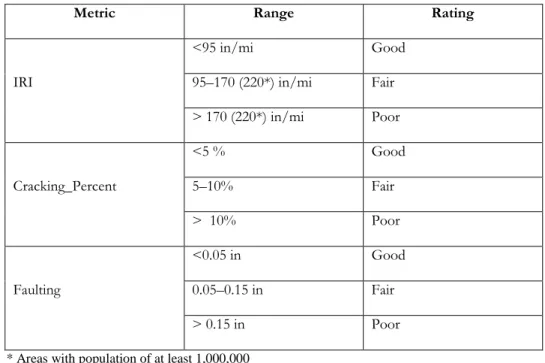
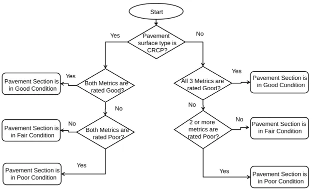
For pavements, each performance metric is rated as Good, Fair, or Poor based on the threshold values shown in Tables 4 through 6. The ratings of these metrics are then combined using the decision tree shown in Figure 4 to determine the performance measures for the pavement section. Each state DOT is required to submit reports on progress in achieving its established targets to the FHWA not later than October 1, 2016, and every two years thereafter.
Table 4-Metrics for Defining Performance Measures for Asphalt Pavement
Metric Range Rating
<95 in/mi Good
IRI 95–170 (220*) in/mi Fair
> 170 (220*) in/mi Poor <5 % Good Cracking_Percent 5–10% Fair > 10% Poor <0.20 in Good Rutting 0.2–0.4 in Fair > 0.40 in Poor
15
Table 5-Metrics for Defining Performance Measures for Jointed Concrete Pavement
Metric Range Rating
<95 in/mi Good
IRI 95–170 (220*) in/mi Fair
> 170 (220*) in/mi Poor <5 % Good Cracking_Percent 5–10% Fair > 10% Poor <0.05 in Good Faulting 0.05–0.15 in Fair > 0.15 in Poor
* Areas with population of at least 1,000,000
Table 6-Metrics for Defining Performance Measures for Continuously Reinforced Concrete
Metric Range Rating
<95 in/mi Good
IRI 95–170 (220*) in/mi Fair
> 170 (220*) in/mi Poor
<5 % Good
Cracking_Percent 5–10% Fair
> 10% Poor
16
Figure 4-Decision Tree for Determining Performance Measure Values for Pavement
The pavement performance measures (as outlined in the January 2015 NPRM) are as follows:
Percentage of pavement lane-miles in good Condition
Percentage of pavement lane-miles in poor Condition
State DOTs can specify separate targets for the National Highway System (NHS) and non-NHS for these performance measures.
While MAP-21 provides the opportunity of evaluating pavement condition nation-wide in a consistent approach, the proposed performance metrics lack clear definitions and may not be available in current pavement management systems. For example, PMIS lacks
No Pavement
surface type is
CRCP?
Start
All 3 Metrics are rated Good? 2 or more metrics are rated Poor? Pavement Section is in Fair Condition Pavement Section is in Good Condition Pavement Section is in Poor Condition
Both Metrics are rated Good? Pavement Section is
in Good Condition
Both Metrics are
rated Poor? Pavement Section is in Fair Condition Pavement Section is in Poor Condition Yes Yes No Yes No No No Yes Yes
17
data on faulting and cracking percent, creating serious difficulties in the implementation of these metrics.
2.3 Pavement Condition Assessment Criteria Used by State DOTs
Most state DOTs use pavement condition indexes as aggregate measures of the structural and material integrity of pavements. While these indexes appear to be similar (essentially a 0–100 scale, with 100 indicating ideal condition), the metrics can have significant difference. To ascertain the level of agreement among these indexes, Papagiannakis et al. (2010) compared six pavement condition indexes used by five state DOTs using actual field data. These indexes are TxDOT’s CS and DS, South Dakota DOT’s surface condition index (SCI), Ohio DOT’s pavement condition rating (PCR), Pennsylvania DOT’s overall pavement index (OPI), and Oregon DOT’s overall index (OI). That study found that significant differences exist among seemingly similar pavement condition indexes.
Table 7 shows the good or better criteria for a sample of state DOTs that use 100-point scale to rate pavement sections, with 100 representing little to no distress situation. Similarly, Table 8 shows the good or better criteria for a sample of state DOTs that use 5-point scale to rate pavement sections.
18
Table 7-Pavement Rating Thresholds Used by State DOTs (100-Point Scale)
State Good or Better Criteria
Georgia 75–100 is good to excellent
Iowa 60–80 is good, 80–100 is excellent
Montana 63–100 is good
Nebraska 70–89 is good; 90–100 is very good
New Hampshire 40–100 is acceptable
North Carolina Greater than 80 is good
Ohio 75–90 is good; 90–100 is very good
Oregon 75.1–98 is good; 98.1–100 is very good
for NHS
Vermont 40–100 is acceptable
Virginia 70–89 is good; greater is excellent
Washington 50–100 is good
Table 8-Pavement Rating Thresholds Used by State DOTs (5-Point Scale)
State Good or Better Criteria
California 2 is good; 1 is excellent
Delaware 3–4 is good; 4–5 is very good
Idaho 3–5 is good
19
Table 8-Continued
State Good or Better Criteria
Michigan 1.0–2.5 is good
New Mexico Greater than 3 is good for Interstate Highways; greater than 2.5 is good for all other highways
Oregon 2.0–2.9 is good; 1.0–1.9 is very good for non-NHS
South Carolina 3.4–4.0 is good; 4.1–5.0 is very good Tennessee 3.5–4.0 is good; 4.0–5 is very good West Virginia 4 is good; 5 is excellent
2.4 Relationship among Performance Metrics
Finding out the relationships among the performance metrics would be very helpful to establish consistent performance targets and to estimate values for metrics from other available ones. Several studies have been conducted to investigate the relationship between IRI and other performance metrics. Al-Omari et al. (1994) conducted a study to explore the correlation between IRI and the Present Serviceability Index (PSR). Abiola et al. (2014) performed a study to investigate the relationship between IRI and a pavement condition score used in Nigeria that combines the density and severity levels of multiple distress types. That study concluded that there is a linear relationship between the two metrics. Park et al. (2007) developed a power regression model which uses IRI to predict
20
the Pavement Condition Index (PCI). Following is the calibrated model suggested by them for the pavement condition data in North Atlantic region:
𝑃𝐶𝐼 = 𝐾1𝐼𝑅𝐼𝐾2 (4)
Using the calibrated model, they developed rating thresholds for IRI based on the already available thresholds for PCI. Gulen et. al (1994) developed regression models between Present Serviceability Index (PSI) and IRI for both concrete and asphalt pavements and find out the critical PSI values for these pavement types in Indiana.
Lin et. al (2003) used an artificial neural network modeling approach to establish a deterioration prediction model for IRI based on the several distress types of the asphalt pavements. The established deterioration model of IRI in terms of each distress type to IRI is as follows:
∆𝐼𝑅𝐼 = 𝐾𝑔𝑝[∆𝐼𝑅𝐼𝑠+ ∆𝐼𝑅𝐼𝑐+ ∆𝐼𝑅𝐼𝑟+ ∆𝐼𝑅𝐼𝑡] + ∆𝐼𝑅𝐼𝑒 (5)
Where:
∆𝐼𝑅𝐼: total incremental change in IRI during the analysis year
∆𝐼𝑅𝐼𝑒: incremental change in IRI due to environment during analysis year
∆𝐼𝑅𝐼𝑠: incremental change in IRI due to structure deterioration during analysis year
21
∆𝐼𝑅𝐼𝑟: incremental change in IRI due to rutting during analysis year
∆𝐼𝑅𝐼𝑡: incremental change in IRI due to potholing during analysis year
𝐾𝑔𝑝: calibration factor
Arhin et. Al (2015) performed a study to predict the pavement condition index using IRI in a dense urban area. They used the 2 years’ data of IRI-PCI to model the relationship between PCI and IRI in Columbia District using a functional classification approach. The main objective of the developed model would be the elimination or a considerable reduction of the time to collect, review and process distress photographs for PCI and thereby the subjective assessment of pavement condition. Their study concluded to the establishment of a linear relationship between IRI and PCI classified by pavement function and pavement types. “The regression models between the IRI and PCI by functional classification and pavement type were determined to be statistically significant within the margin of error (5% level of significance), with R2 values between 0.56 and 0.82. The results of the ANOVA tests also showed statistically significant F - statistics (p < 0.05) in addition to statistically significant regression coefficients (from the t-tests, with p < 0.05). The residual plots for all the models also showed randomness about the zero line indicating their viability, in addition to the normal probability plots showing points near a straight line.”
This research investigates various statistical models to establish a reasonable relationship between CS, DS, and IRI.
22
2.5 Pavement Performance in Urban and Rural Areas
In the MAP-21 rulemaking (FHWA 2015) and other sources in the literature (for example, La Torre et al. 2002), different performance threshold values are used for assessing the performance of pavements in urban and rural areas. This delineation between urbanized and non-urbanized roads is based on the recognition that urbanized roads have distinct characteristics compared to rural roads that affect their pavement condition and the user’s perception of these condition, such as varying lane width and configuration, traffic flow, and the presence of utility cuts (Shahin et al. 2003). In MAP-21, the term non-urbanized is defined to include rural areas as well as small urban areas that do not have all the characteristics of urbanized areas. The Federal Highway Administration (FHWA) has proposed that urban boundaries be identified through the most recent U.S. Decennial Census.
A number of studies have been conducted previously to understand and quantify the differences in the performance of pavements in urban and rural areas. However, much of that literature has focused on ride quality. Prior to MAP-21, the literature recognized the differences between urban and rural roads in terms of roughness acceptability and roadway characteristics. One of the early studies in this area was conducted by La Torre et al. (2002) to investigate the correlation between pavement roughness and user perception in an urban area. The study found that urban drivers have higher tolerance for road roughness than rural divers. Also, that study developed a modified IRI (called IRI*) for measuring roughness of urban roads in Italy (La Torre at al. 2002). IRI* was developed to account for differences between urban roads and rural roads (e.g., lower speed, shorter
23
pavement management sections, that different pavement types). Namur et al. (2009) addressed the issues involved in using IRI to measure roughness of unpaved rural roads. They concluded that conventional techniques of pavement roughness measurement are not appropriate for unpaved roads and suggested the use of visual inspection data to estimate IRI through correlations between IRI and various distress. Osorio et al. (2014) developed statistical models for measuring the condition of urban pavements as a function of distresses relevant to these types of pavements.
This study focuses on measuring the performance differences between urban and rural roads using a large set of historical data that include both ride quality and distresses. United States Census Bureau has been using different criteria since 1910 to delineate the urban and rural areas. From 1910 Census to 1940 Census, the term “urban” was referred to any incorporated area containing at 2,500 people within its boundaries (DOC 2010). Census Bureau adopted the concept of “Urbanized Areas (UA)” for the 1950 Census due to the increasing rate of suburbanization outside the boundaries of incorporated urban areas. Consequently, “Urban” was defined as any territory, persons and housing units in incorporated or unincorporated areas inside urbanized areas or outside urbanized areas with more than 2,500 people (DOC 2010). This criterion to delineate urban and rural areas remained unchanged until Census 2000. Considering the possibility of having a densely settled area outside of an urban area’s boundaries with as much “urbanized features” as for those areas inside the boundaries, led to the definition of “Urban Clusters” after 2000 Census. Therefore, the Census Bureau identifies two types of urban areas:
24
Urbanized Areas (UAs) of 50,000 or more people;
Urban Clusters (UCs) of at least 2,500 and less than 50,000 people. Based on the above definitions, the flowing criteria was defined to delineate the urban areas for Census 2000:
“For Census 2000, the Census Bureau classifies as "urban" all territory, population, and housing units located within an urbanized area (UA) or an urban cluster (UC). It delineates UA and UC boundaries to encompass densely settled territory, which consists of:
core census block groups or blocks that have a population density of at least 1,000 people per square mile and
surrounding census blocks that have an overall density of at least 500 people per square mile
In addition, under certain conditions, less densely settled territory may be part of each UA or UC.”
“For the 2010 Census, an urban area will comprise a densely settled core of census tracts and/or census blocks that meet minimum population density requirements, along with adjacent territory containing non-residential urban land uses as well as territory with low population density included to link outlying densely settled territory with the densely settled core. To qualify as an urban area, the territory identified according to criteria must encompass at least 2,500 people, at least 1,500 of which reside outside institutional group quarters.”
25
"Rural" encompasses all population, housing, and territory not included within an urban area.” (DOC 2010)
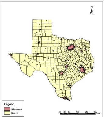
Based on this definitions, Census Bureau has developed a geographical database on a GIS platform to delineate the boundaries of urban areas. This geographical database was used through this study to delineate between urban and rural areas according to the MAP-21’s proposed urban and rural delineation criteria based on the most recent U.S. Decennial Census (Census 2010) [5]. Figure 5 is a graphical indication of the identified urban areas throughout the State of Texas in year 2014 based on the Census 2010 criteria. Using the geoprocessing tools of ArcMAP, the urban areas within the Houston District can be extracted and used for this study.
26
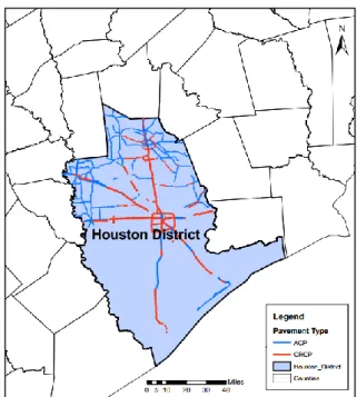
As discussed earlier, currently, about six percent of TxDOT’s roadway lane-miles is CRCP, about one percent is jointed concrete pavement (JCP), and about 93 percent is asphalt-surfaced pavement. This section analyzes the performance of CRCP and ACP in the Houston District based on three performance metrics used by TxDOT or proposed in MAP-21 rules. The map shown in Figure 6 displays these pavements in the Houston District. JCP is not considered in this analysis due to the very limited use of this pavement type in Texas.
Figure 6-Map of CRCP and ACP Sections in the Houston District
* Part of the data reported in this chapter is reprinted with permission from “CRCP Performance Patterns Gleaned from Texas Pavement Management Data” by Authors Litao Liu, Amir Rashed, and Nasir G. Gharaibeh, 2016. 11th International Conference on Concrete Pavements, San Antonio, Texas, USA
27
3.1 CRCP Design and Management Practices in Texas
CRCP is a Portland Cement Concrete (PCC) pavement with continuous longitudinal reinforcement and without any transverse expansion or contraction joints. (PMIS Rater’s Manual 2014). CRCP pavements are stored with code “01” in PMIS database as the detailed pavement type code.
Currently, the only officially approved design method for CRCP by TxDOT is the 1993 AASHTO Guide for Design of Pavement Structures. Typical input values used by TxDOT for this design method are shown in Table 9.
Previously, the concrete slab thickness required by TxDOT had a range between 8 inches and 15 inches. Currently, the design standard used by TxDOT specifies that the thickness of CRCP slab should be 6 inches to 13 inches. Thickness values outside this range need to be submitted to the District Engineer for approval along with justification.
TxDOT requires one of the following base layer combinations for concrete slab support:
4-inch asphalt concrete pavement or asphalt stabilized base, or
A minimum 1-inch asphalt concrete bond breaker over 6-inch cement stabilized base.
Tied PCC shoulders are normally used with CRCP. The width of shoulders varies from 2 to 10 feet, depending on the functional classification of the roadway under design. The PCC shoulder should have the same thickness and the same base layers as the main-lane pavement.
28
Table 9-Input Variables and Design Values Used in TxDOT CRCP Design
Input Variable TxDOT Design Value
28-day concrete modulus of rupture, psi 620 28-day concrete elastic modulus, psi 5,000,000 Effective modulus of subgrade reaction,
psi/in
300 – 700
Serviceability indices 4.5 (initial) – 2.5 (terminal)
Drainage coefficient
0.91 – 0.95 for annual rainfall 58 – 50 in.
0.96 – 1.00 for annual rainfall 49 – 40 in.
1.01 – 1.05 for annual rainfall 39 – 30 in.
1.06 – 1.10 for annual rainfall 29 – 20 in.
1.11 – 1.16 for annual rainfall 19 – 8 in.
Overall standard deviation 0.39
Reliability, %
95% for > 5 million design ESALs 90% for 5 million design ESALs
18-kip equivalent single axle load (ESAL)
Based on the traffic analysis report provided by the Transportation Planning and
Programming Division
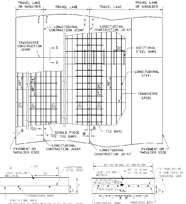
Figure 7 shows a typical CRCP pavement layout and Table 10 shows the longitudinal steel design for CRCP in Texas.
29
Figure 7-Typical CRCP Slab and Construction Joint Layout (Texas Department of Transportation (TxDOT), (2013), Continuously Reinforced Concrete Pavement
One Layer Steel Bar Placement, CRCP (1)-13)
Section Y - Y Section X - X
30
Table 10-Longitudinal Steel Design
Slab Thickness, in. Steel Bar Size Steel Bar Spacing, in. First Spacing at Edge or Joint, in.
Additional Steel Bars at Transverse Construction
Joint
Spacing, in. Length, in.
7.0 #5 6.5 3 to 4 13 50 7.5 #5 6.0 3 to 4 12 50 8.0 #6 9.0 3 to 4 18 50 8.5 #6 8.5 3 to 4 17 50 9.0 #6 8.0 3 to 4 16 50 9.5 #6 7.5 3 to 4 15 50 10.0 #6 7.0 3 to 4 14 50 10.5 #6 6.75 3 to 4 13.5 50 11.0 #6 6.5 3 to 4 13 50 11.5 #6 6.25 3 to 4 12.5 50 12.0 #6 6.0 3 to 4 12 50 12.5 #6 5.75 3 to 4 11.5 50 13.0 #6 5.5 3 to 4 11 50
Unit Conversions: 1 inch = 25.4 mm.
3.2 ACP Design and Management Practices in Texas
The asphalt-surfaced pavement category includes both Asphalt Concrete Pavement (ACP) and old Portland Cement Concrete (PCC) pavement that has been
31
overlaid with hot-mix asphalt. As mentioned earlier, about 93% of TxDOT’s lane-miles is asphalt-surfaced pavements. Asphalt-surfaced pavements are stored with one of the codes “04” through “09” in the PMIS database indicating the detailed pavement type. The following are the descriptions these codes:
04: Thick Asphaltic Concrete (Over 5.5")
05: Medium Thickness Asphaltic Concrete (2.5 - 5.5") 06: Thin Asphaltic Concrete (Under 2.5")
07: Composite (Asphalt Surfaced Concrete) 08: Widened Composite Pavement
09: Overlaid and Widened Asphaltic Concrete Pavement 10: Surface Treatment Pavement (Or Seal Coat)
Currently, TxDOT accepts the following methods for designing flexible pavements:
FPS-19W for flexible pavements
AASHTO design procedure (1993)
Modified Texas Triaxial Design Method for flexible pavements Each method is briefly explained through the following sections.
TxDOT considers FPS-19W as the preferred method for designing of flexible pavements (especially for high volume highways). FPS-19W uses a mechanistic-empirical design procedure which is suggested to be used as a check for the design of all flexible pavements. Table 11 displays the five design types used by FPS-19W.
32
Table 11-FPS-19W Five Basic Design Types
1 2 3 4 5
HMA or Surface Treatment
HMA HMA HMA HMA Overlay
Flexible Base Asphalt Stabilized Base
Asphalt Stabilized Base
Flexible Base Existing HMA
Subgrade Subgrade Flexible Base Stabilized Subbase/ Subgrade
Existing Base
Subgrade Subgrade Subgrade
The AASHTO 1993 Design Procedure is an empirical method that uses the concepts of Structural Number (SN). Structural Number is sum of a layer coefficient (a), layer thickness (D) and drainage coefficient (m) for each layer. (see equation 6)
𝑆𝑁 = 𝑎1𝐷1+ 𝑎2𝐷2𝑚2+ 𝑎3𝐷3𝑚3+ ⋯ (6)
The Modified Texas Triaxial design method uses the concept of the Texas Triaxial Classification of soils which was developed in 1940s. This method requires the use of subgrade or base Texas Triaxial class derived from laboratory test results. During recent
33
years, this method has been automated and incorporated into the FPS-19W program as a post-design check modulus.
3.3 Performance of Pavements in Houston District 3.3.1 IRI
The PMIS database contains separate fields for IRI in the right wheel-path and IRI in the left wheel-path. The IRI values used in this study are the average IRI of the left and right wheel paths.
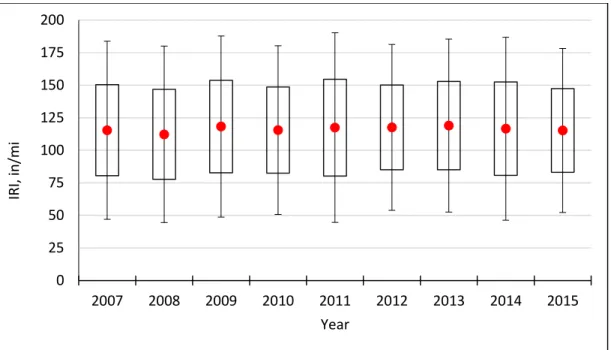
The box and whisker diagram depicted in Figure 8 shows that the IRI of the middle 68 percent of CRCP lane-miles in the Houston District consistently ranged between about 80 in/mi and 150 in/mi (with a mean value of approximately 120 in/mile) over the past nine years (2007-2015). Figure 9 shows that the IRI of the middle 68 percent of ACP lane-miles in the Houston District consistently ranged between about 50 in/mi and 120 in/mi (with a mean value of approximately 82 in/mile) over the past nine years (2007-2015).
34
Figure 8-Box and Whisker Diagrams for CRCP IRI in the Houston District (Whiskers = 95% Confidence Interval; Solid Circle=Mean; Box = 68% Confidence
Interval)
Figure 9-Box and Whisker Diagrams for ACP IRI in the Houston District (Whiskers = 95% Confidence Interval; Solid Circle=Mean; Box = 68% Confidence
Interval) 0 25 50 75 100 125 150 175 200 2007 2008 2009 2010 2011 2012 2013 2014 2015 IRI, in /m i Year 0 25 50 75 100 125 150 175 200 2007 2008 2009 2010 2011 2012 2013 2014 2015 IRI, in /m i Year
35
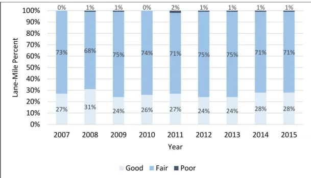
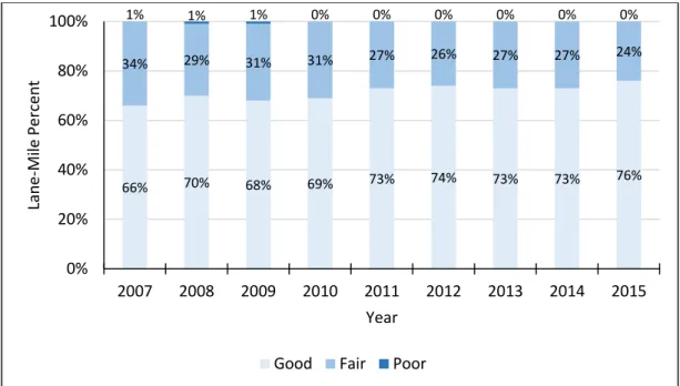
Using the IRI thresholds proposed in the January 2015 NPRM of MAP-21, the majority of CRCP lane-miles would be classified as Fair and approximately 25 percent would be classified as Good (see Figure 10). Only less than one percent would be classified as Poor. On the other hand, the majority of ACP lane-miles would be classified as Good; approximately 35 percent would be classified as Fair; and less than one percent would be classified as Poor during the past nine years (Figure 11).
Figure 10-CRCP Performance in the Houston District Based on IRI Thresholds Proposed in the January 2015 NPRM of MAP-21
27% 31% 24% 26% 27% 24% 24% 28% 28% 73% 68% 75% 74% 71% 75% 75% 71% 71% 0% 1% 1% 0% 2% 1% 1% 1% 1% 0% 10% 20% 30% 40% 50% 60% 70% 80% 90% 100% 2007 2008 2009 2010 2011 2012 2013 2014 2015 Lan e -Mi le P er cent Year Good Fair Poor
36
Figure 11-ACP Performance in the Houston District Based on IRI Thresholds Proposed in the January 2015 NPRM of MAP-21
3.3.1.1 Statistical Analysis of IRI Data
To further investigate the differences between the performance of different pavement types in Houston District, a t-test for samples with unequal variances is conducted on each pair of annual IRI data using a statistical analysis software, JMP. The null hypothesis and alternative hypothesis for this test are formulated as follows:
Null Hypothesis H0: μ1 = μ2 (means are equal) Alternative Hypothesis H1: μ1 ≠ μ2 (means are not equal)
66% 70% 68% 69% 73% 74% 73% 73% 76% 34% 29% 31% 31% 27% 26% 27% 27% 24% 1% 1% 1% 0% 0% 0% 0% 0% 0% 0% 20% 40% 60% 80% 100% 2007 2008 2009 2010 2011 2012 2013 2014 2015 Lan e -Mi le P er cent Year Good Fair Poor
37 This test uses the following t-statistic:
Tγ = X1 ̅̅̅ − X̅̅̅2 √S12 N1 +S2 2 N2 (7)
X1 and X2 are sample means, S1 and S2 are sample standard deviations, N1 and N2 represent the sample sizes and γ is the t-distribution’s degree of freedom. The degree of freedom for this test is estimated using the Welch-Satterthwaite equation:
γ = (S12 N1 + S22 N2) 2 (S12 N1) 2 N1− 1 + (S22 N2) 2 N2− 1 (8)
Testing for the equality of means, the two-tailed P-Value is derived as the probability of getting an extreme value against the null hypothesis. This is computed as follows:
38
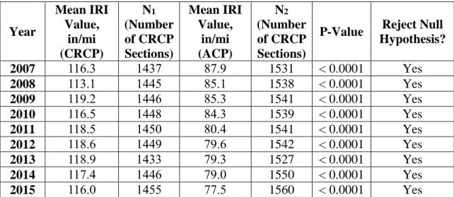
Applying the test on each pair of annual IRI data with a significance level of 0.05, the null hypothesis is rejected if resulting P-Value is less than 0.05. The results of the hypothesis tests are summarized in Table 12. The table also includes the average annual IRI values of urban and rural pavements and the P-Values of the test.
Table 12 shows that the null hypothesis is rejected for all annual data of IRI tests. This supports the fact of a significant difference between the behavior of CRCP and ACP sections in Houston District.
Table 12-Hypothesis Testing of Difference in Performance Between CRCP and ACP Based on IRI
Year Mean IRI Value, in/mi (CRCP) N1 (Number of CRCP Sections) Mean IRI Value, in/mi (ACP) N2 (Number of CRCP Sections)
P-Value Reject Null Hypothesis? 2007 116.3 1437 87.9 1531 < 0.0001 Yes 2008 113.1 1445 85.1 1538 < 0.0001 Yes 2009 119.2 1446 85.3 1541 < 0.0001 Yes 2010 116.5 1448 84.3 1539 < 0.0001 Yes 2011 118.5 1450 80.4 1541 < 0.0001 Yes 2012 118.6 1449 79.6 1542 < 0.0001 Yes 2013 118.9 1433 79.3 1527 < 0.0001 Yes 2014 117.4 1446 79.0 1550 < 0.0001 Yes 2015 116.0 1455 77.5 1560 < 0.0001 Yes 3.3.2 Distress Score
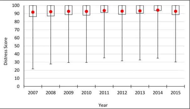
The DS box and whisker diagram, depicted in Figure 12, shows that the DS of 68 percent of CRCP lane-miles in the Houston District consistently ranged between about 85 and 100 (with a mean value of approximately 92) over the past nine years (2007-2015).
39
On the other hand, Figure 13 shows that the DS of 68 percent of ACP lane-miles in the Houston District has had a considerable variation during three consecutive years from 2009 to 2011. During this period the DS of 68 percent of ACP lane-miles has ranged between 65 and 100 (with a mean value of approximately 82). Other annual data show similar results to those of CRCP with a mean value of approximately 90.
Figure 12-Box and Whisker Diagrams for CRCP DS in the Houston District (Whiskers = 95% Confidence Interval; Solid Circle=Mean; Box = 68% Confidence
Interval) 0 10 20 30 40 50 60 70 80 90 100 2007 2008 2009 2010 2011 2012 2013 2014 2015 Di st ress S co re Year
40
Figure 13-Box and Whisker Diagrams for ACP DS in the Houston District (Whiskers = 95% Confidence Interval; Solid Circle=Mean; Box = 68% Confidence
Interval)
Using the DS threshold values specified by TxDOT, the majority (approximately 89 percent) of CRCP lane-miles would be classified as Good or Very Good, approximately three percent as Fair, and approximately eight percent as Poor (see Figure 14). Using the DS threshold values specified by TxDOT, the majority (62 percent to 88 percent on different years) of ACP lane-miles would be classified as Good or Very Good, approximately three percent as Fair. The percentage of lane-miles classified as poor are considerable between 2009 and 2011 which ranges between 26 percent and 30 percent. For the other annual data approximately eight percent of lane-miles would be classified as Poor (see Figure 15).
0 10 20 30 40 50 60 70 80 90 100 2007 2008 2009 2010 2011 2012 2013 2014 2015 Di st ress S co re Year
41
Figure 14-CRCP Performance in the Houston District Based on DS Thresholds Specified by TxDOT
Figure 15-ACP Performance in the Houston District Based on DS Thresholds Specified by TxDOT 87% 87% 89% 88% 90% 89% 89% 90% 88% 2% 4% 2% 2% 2% 2% 3% 2% 3% 11% 9% 9% 10% 8% 8% 8% 8% 9% 0% 20% 40% 60% 80% 100% 2007 2008 2009 2010 2011 2012 2013 2014 2015 Lan e -Mi le P er cent Year
Good or Very Good Fair Poor or Very Poor
84% 80% 66% 62% 65% 80% 88% 86% 84% 4% 7% 8% 8% 7% 6% 5% 6% 7% 12% 13% 26% 30% 28% 14% 7% 8% 8% 0% 20% 40% 60% 80% 100% 2007 2008 2009 2010 2011 2012 2013 2014 2015 Lan e -Mi le P er cent Year
42 3.3.2.1 Statistical Analysis of Distress Score Data
To further analyze the difference between DS of different pavement types in Houston District, the same procedure and software used for statistical analysis of IRI are applied to DS. The results of the hypothesis tests are summarized in Table 13.
The null hypothesis for DS t-tests is rejected for six of the past nine years and is accepted for the other three years (2007, 2013 and 2015). Considering that the hypothesis of equal means is rejected for about 70 percent of the time (i.e. 6 out of 9 years), this test also makes a weaker evidence to conclude that there is a significant difference in the performance of different pavement types in Houston District based on their distresses.
Table 13-Hypothesis Testing of Difference in Performance Between CRCP and ACP Based on DS Year Mean DS Value (CRCP) N1 (Number of CRCP Sections) Mean DS Value (ACP) N2 (Number of ACP Sections)
P-Value Reject Null Hypothesis? 2007 92.7 1273 92.7 1501 0.9666 No 2008 92.8 1328 91.5 1540 0.0453 Yes 2009 93.2 1352 82.5 1538 < 0.0001 Yes 2010 93.1 1404 82.2 1544 < 0.0001 Yes 2011 94.0 1435 83.9 1544 < 0.0001 Yes 2012 93.4 1428 89.1 1541 < 0.0001 Yes 2013 93.5 1449 94.1 1529 0.3366 No 2014 94.8 1452 93.1 1539 0.0012 Yes 2015 93.2 1455 92.4 1560 0.1864 No
43 3.3.3 Condition Score
The CS box and whisker diagram, depicted in Figure 16, shows that the CS of 68 percent of CRCP lane-miles in the Houston District consistently ranged between about 75 and 100 (with a mean value of approximately 90) over the past nine years (2007-2015). The CS box and whisker diagram, depicted in Figure 17, shows that except for the annual data from 2009 to 2011, the CS of 68 percent of ACP lane-miles in the Houston District consistently ranged between about 75 and 100 (with a mean value of approximately 90) over the past nine years (2007-2015). The lower bottom of the boxes for CS of 68 percent of ACP lane-miles from 2009 to 2011 has dropped to 65 with a mean value of approximately 85.
Figure 16-Box and Whisker Diagrams for CRCP CS in the Houston District (Whiskers = 95% Confidence Interval; Solid Circle=Mean; Box = 68% Confidence
Interval) 0 10 20 30 40 50 60 70 80 90 100 2007 2008 2009 2010 2011 2012 2013 2014 2015 Co nd it io n S co re Year
44
Figure 17-Box and Whisker Diagrams for ACP CS in the Houston District (Whiskers = 95% Confidence Interval; Solid Circle=Mean; Box = 68% Confidence
Interval)
Using the CS threshold values specified by TxDOT, the majority (approximately 85 percent) of CRCP lane-miles would be classified as Good or Very Good, approximately seven percent as Fair, and approximately eight percent as Poor (see Figure 18). On the other hand, the majority (varied from 70 percent to 90 percent) of ACP lane-miles would be classified as Good or Very Good, approximately 10 percent to 24 percent as Fair, and approximately two percent as Poor (see Figure 19).
0 10 20 30 40 50 60 70 80 90 100 2007 2008 2009 2010 2011 2012 2013 2014 2015 Co nd it io n S co re Year
45
Figure 18-CRCP Performance in the Houston District Based on CS Thresholds Specified by TxDOT
Figure 19-ACP Performance in the Houston District Based on CS Thresholds Specified by TxDOT 85% 86% 84% 85% 84% 85% 84% 87% 86% 6% 6% 7% 8% 7% 8% 8% 6% 7% 9% 8% 9% 7% 9% 7% 7% 7% 7% 0% 10% 20% 30% 40% 50% 60% 70% 80% 90% 100% 2007 2008 2009 2010 2011 2012 2013 2014 2015 La ne -Mi le Per cen t Year
Good or Very Good Fair Poor or Very Poor
86% 84% 72% 69% 71% 84% 92% 89% 91% 9% 11% 23% 24% 23% 12% 6% 9% 8% 5% 4% 5% 6% 6% 4% 2% 2% 1% 0% 20% 40% 60% 80% 100% 2007 2008 2009 2010 2011 2012 2013 2014 2015 Lan e -Mi le P er cent Year
46
3.3.3.1 Statistical Analysis of Condition Score Data
To further analyze the difference between CS of different pavement types, the same procedure and software used for statistical analysis of IRI and DS are applied to CS. The results of the hypothesis tests are summarized in Table 14.
The null hypothesis for CS t-tests is rejected for six of the past nine years and is accepted for the other three consecutive years (2009, 2010, and 2011). Considering that the hypothesis of equal means cannot be rejected for 30 percent of the time (i.e. 3 out of 9 years), this test makes a weaker evidence to conclude that there is a significant difference in the performance of different pavement types based on their distresses.
Table 14-Hypothesis Testing of Difference in Performance Between CRCP and ACP Based on CS Year Mean CS Value (CRCP) N1 (Number of CRCP Sections) Mean CS Value (ACP) N2 (Number of ACP Sections)
P-Value Reject Null Hypothesis? 2007 87.9 1255 90.8 1448 0.0004 Yes 2008 88.4 1318 90.1 1481 0.0260 Yes 2009 87.1 1343 81.5 1376 < 0.0001 No 2010 87.4 1397 81.3 1490 < 0.0001 No 2011 86.8 1430 83.1 1493 < 0.0001 No 2012 87.0 1422 88.3 1485 0.0994 Yes 2013 86.9 1429 93.6 1477 < 0.0001 Yes 2014 88.7 1443 92.0 1489 < 0.0001 Yes 2015 87.7 1455 91.4 1511 < 0.0001 Yes
47
3.4 Consistency among Performance Metrics for ACP and CRCP
As summarized in Table 15, IRI and DS agreed about 67 percent of the time (i.e. 6 years out of 9 study years) when comparing the performance of ACP and CRCP. Similar agreement was found between IRI and CS. However, DS and CS agreed about 33.3 percent of the time (i.e. 3 years out of 9 study years) when comparing the performance of ACP and CRCP. The three metrics agreed about 33.3 percent of the time (i.e. 3 years out of 9 study years).
Table 15-Summary of Hypothesis Test Results for CRCP and ACP
Year Reject Null Hypothesis based on IRI? Reject Null Hypothesis based on DS? Reject Null Hypothesis based on CS? 2007 Yes No Yes
2008 Yes Yes Yes
2009 Yes Yes No
2010 Yes Yes No
2011 Yes Yes No
2012 Yes Yes Yes
2013 Yes No Yes
2014 Yes Yes Yes
48
This section investigates the differences between the performance of roadway pavements in urban and rural areas based on IRI, CS, and DS. In this study, urban areas are defined as all densely settled core of census tracts and/or census blocks with minimum population of 2,500 people. Generally, a census block is the smallest geographic unit for which the Census Bureau tabulates decennial census data. In cities, many census blocks correspond to individual city blocks bounded by streets. Rural areas are areas that do not meet the definition of an urban area (DOC 2010).
4.1 Delineation of Urban and Rural Areas in Houston District
Using the Census 2010 criteria for delineation between the urban and rural areas, U.S. Census Bureau has created a geographic shapefile for graphically representation of the urban boundaries of the country for year 2014. The geographic representation of urban areas of year 2014 was used through this research to distinguish between the urban and rural areas. Figure 20, displays the urban boundaries in Houston District gleaned from this database.
49
Figure 20-Urban and Rural Areas in Houston District
By identifying the urban and rural areas in Houston District, next step is to classify the pavement sections based on their location. In order to achieve this goal, the “clip” geoprocessing tool in ArcMAP is used to clip the pavement sections using the urban boundaries. Section lengths are updated afterward to obtain the new lengths for those pavements laying in both urban and rural areas. Figure 21 is a graphical indication of the urban and rural pavement sections obtained after this step:
50
Figure 21-Urban and Rural Roads in Houston District
4.2 Performance of Pavements in Urban and Rural Areas
Next step after classifying pavements into urban and rural roads is to evaluate the performance of pavement in suggested urban or rural areas. Following sections include the performance assessment results of urban and rural pavements based on IRI, DS and CS and the statistical analysis to investigate the possible differences between their behaviors.