Interpolation for De-Dopplerisation
W R Graham
University of Cambridge, Department of Engineering, Trumpington Street, Cambridge, CB2 1PZ
Abstract
‘De-Dopplerisation’ is one aspect of a problem frequently encountered in experimental acoustics: deducing an emitted source signal from received data. It is necessary when source and receiver are in relative motion, and requires interpolation of the measured signal. This introduces error. In acoustics, typical current practice is to employ linear interpolation and reduce error by over-sampling. In other applications, more advanced approaches with better performance have been developed. Associated with this work is a large body of theoretical analysis, much of which is highly specialised. Nonetheless, a simple and compact performance metric is available: the Fourier transform of the ‘kernel’ function underlying the interpolation method. Furthermore, in the acous-tics context, it is a more appropriate indicator than other, more abstract, candidates. On this basis, interpolators from three families previously identified as promising — piecewise-polynomial, windowed-sinc, and B-spline-based — are compared. The results show that significant improve-ments over linear interpolation can straightforwardly be obtained. The recommended approach is B-spline-based interpolation, which performs best irrespective of accuracy specification. Its only drawback is a pre-filtering requirement, which represents an additional implementation cost com-pared to other methods. If this cost is unacceptable, and aliasing errors (on re-sampling) up to approximately 1% can be tolerated, a family of piecewise-cubic interpolators provides the best alternative.
Keywords: Doppler effect, acoustic signal processing, acoustic measurement
1. Introduction
The Doppler effect is a well-known feature of wave propagation; it occurs when there is relative motion between a source and its observer. The corresponding variation in propagation distance means that pulses emitted by the source at a given rate arrive at the observer at an altered rate. The difference is known as the Doppler frequency shift.
In acoustics applications, one typically wishes to characterise a source via measurements of its associated sound field. The acoustic pressure at location x and time t due to a moving source is a function of x and the time te when the sound was emitted [1, Ch. 14]. Given the path of the
source, the link betweente and t can be calculated. Hence, in principle, the required information
— the source strength as a function of emission time — can be deduced. In practice, however, the measurement is made at discrete, uniformly spaced, instants; hence the source strength can only be estimated at the corresponding emission times, and these will be at varying intervals. Further analysis of the source signal almost always requires regularly sampled values, which must be derived by interpolation. This process was denoted ‘de-Dopplerization’ by Howell et al. [2], who applied
it to aircraft flyover noise measurements. Its relevance to measurements of ground transportation noise was also recognised around the same time [3, 4].
The question of accuracy in the interpolation was addressed in an ad hoc manner by Howell et al. [2]. They considered two possible algorithms — nearest-neighbour and linear — and analysed a simulated signal consisting of band-limited random noise. The signal-to-noise ratio was then determined on the basis of the (spurious) spectrum level of the interpolated signal outside the original noise band. Linear interpolation was found to be clearly superior to nearest-neighbour approximation, but over-sampling of the ‘measured’ signal was necessary to obtain satisfactory accuracy. (For a signal spanning 1200-1800Hz, sampled at 5kHz, the signal-to-noise ratio was only 20dB. This increased to 35dB when the signal sample rate was doubled, leaving the output rate at 5kHz.) Barsikow and King [3] also recognised the need for over-sampling; in their case they acquired data at nine times the Nyquist-criterion value and used nearest-neighbour approximation. Finally, Usagawa et al. [4] proposed a more sophisticated interpolation based on a cubic-spline fit, but still concluded that a raised sampling rate was necessary.
Subsequently, the prospect of improved interpolation approaches was raised by Glegg [5], who observed that the linearly-interpolated and re-sampled signal could be viewed as the result of passing the original measurement through a (non-linear) digital filter. On the basis of the root-mean-square error for sinusoidal inputs, Glegg showed that higher-order filters could reduce the degree of over-sampling needed. Higher-order interpolation, based on local cubic fitting, was also employed by Ludecke [6]. Nonetheless, over-sampling and linear interpolation have remained in use [7, 8], and form the basis of the present-day ROSI algorithm [9, 10].
Meanwhile, in the field of image processing, interpolation methods have been intensively stud-ied, and have become much better understood. The fundamental insight underlying this work follows from the expression of the interpolated function,fi, as a convolution of the discrete sample
values with a ‘kernel’ functionh:
fi(t) =
∞
X
n=−∞
h(t/T −n)f(nT). (1)
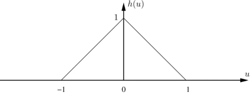
Here, given the context, we take the independent variable to be time,t. The original functionf(t) is sampled with spacing T, and the kernel function is defined in a form independent of sampling frequency. As a concrete example, consider linear interpolation. In this case,his the ‘tent’ function shown in Fig. 1, and given by
h(u) = 1− |u|, |u|<1;
= 0, |u| ≥1. (2)
Note that the interpolated function defined by Eq. (1) is not discrete; it exists for all values of t. In practice, it must be re-sampled for subsequent use, but this intermediate form is extremely useful. Specifically, it is linear; the non-linearity noted by Glegg [5] is only introduced by re-sampling. It follows that the Fourier transform is the product of the transforms of the kernel and the sampled function. This observation allows important, and universal, accuracy information to be derived from the kernel transform alone. Specifically, the kernel performance can be assessed against the ideal interpolator transform, which passes (without attenuation) all frequencies below Nyquist and rejects all frequencies above. (The latter are introduced by the sampling process, even if the measured signalf(t) is band-limited.)
1
−1 0
1
h(u)
u
Figure 1: The interpolatorh(u) corresponding to linear interpolation.
In an influential early work, Keys [11] showed that a piecewise-cubic form forh(u), non-zero for |u|< 2, had a more favourable Fourier transform than nearest-neighbour or linear interpolators. However, the move to higher-order polynomials introduces complexity; whereas the tent function of Fig. 1 is uniquely determined by the requirement that sample values are replicated by Eq. (1), the piecewise cubic is not. Keys additionally specified value and gradient continuity, and the ability to reproduce a sampled quadratic exactly, but other criteria are also possible. For example, Schaum [12] suggested ‘low-frequency’ interpolators that maximise the degree of polynomial which can be reproduced and sacrifice the continuity requirements. Schaum also introduced an error measure, assuming interpolation and subsequent re-sampling at the same rate but at shifted positions, and used it to assess a number of potential interpolators.
Similar, but more recent and extensive, reviews have been published by Lehmann et al. [13] and Th´evenaz et al. [14]. Both include considerations of numerical cost; the former judges accuracy on the basis of the interpolator’s Fourier transform and its performance in numerical experiments chosen to typify medical imaging requirements; the latter employs a spectral error measure first introduced by Park and Schowengerdt [15]. Recommendations arising from these studies are a novel cubic interpolator [13] and a cubic-spline fit [14].
In summary, it is clearly possible to improve significantly on linear interpolation. One could, nonetheless, argue that its simplicity makes the associated over-sampling requirement a price worth paying. This view might be tenable for the two-fold increase suggested by Howell et al. [2] on the basis of their background-noise estimate. However, this ignores signal attenuation, consideration of which leads to far greater multiples [8]. Hence we argue that more sophisticated methods should be employed. The question then is: which should be chosen? Interpolation research has provided many options but, as yet, no unqualified consensus on an optimal approach. Even where recommendations are available, they are made in the context of image processing. The aim of the current work is to provide concrete guidance for appropriate choices in acoustics applications. In doing so, it will be assumed that data sets are large, and are straightforwardly extendable at beginning and end by increasing acquisition time. The first feature applies also in image processing, and implies that computational efficiency is a consideration. The second is not typical of image data, and means that ‘edge effects’ are of less concern here.
The paper has three main sections. The first reviews interpolator theory, in order to explain why the Fourier transform of h(u) is the appropriate comparison metric. Readers prepared to accept this point without further justification can skip to Section 3, which investigates the characteristics of a range of interpolators from three different families, and identifies preferred members from
each. Section 4 then presents a comparison of the different types, and recommendations for which to choose. Readers solely interested in the latter can confine themselves to this part of the paper.
2. Background theory
Here the theoretical considerations underlying interpolator design and assessment are intro-duced. The material presented is not novel; it is drawn from the signal-processing literature. However, even review papers in the field assume significant prior knowledge, and the underlying works often derive their results with greater generality (hence, also, complexity) than is necessary for our purposes. Thus the aim is to give a complete, self-contained, account of the theory that is directly relevant to interpolation in our context. For the sake of accessibility, no attempt is made to reproduce the mathematical rigour of the original sources.
2.1. Assumptions and restrictions
Consider first the measured signal. We assume that it is band-limited, and has been uniformly sampled at a frequency high enough to avoid aliasing.
The interpolated signal is given by Eq. (1). As noted previously, this continuous function must be re-sampled at some stage. However, it fully characterises the implications of the interpolation method, and hence is the most transparent representation to study. Furthermore, as will be seen, an understanding of its properties leads directly to straightforward requirements for re-sampling.
Turning to the kernel function,h, we restrict attention to genuine interpolators, i.e. those which exactly reproduce the values of the sampled signal whentcoincides with a sample time, nT. This implies, for integerk,
h(k) = 1, k= 0;
= 0, otherwise. (3)
(Although natural, this constraint excludes the possibility of combining interpolation with another operation, such as smoothing. The viewpoint taken here is that clarity in data processing is best achieved when each desired operation is carried out separately.) The other constraint on the interpolator is that it should be symmetric:
h(−u) =h(u). (4)
This requirement is intuitively self-evident. Its benefit in mathematical terms will become clear subsequently.
2.2. Frequency-domain representation
The starting point for the theoretical analysis of interpolation is the Fourier transform of the interpolated function:
Fi(ω) = Z ∞
−∞
fi(t)e−iωtdt. (5)
fi(t) = ∞ X n=−∞ Z ∞ −∞ f(uT)h t T −u δ(u−n) du, (6)
and then substituting the Fourier-series representation for P
nδ(u−n) derived in Appendix A.1.
This allows Eq. (5) to be manipulated into the form Fi(ω) =H(ωT)
∞
X
m=−∞
F(ω−mωs), (7)
in which: ωsis the radian sampling frequency, 2π/T;F(ω) is the Fourier transform off(t), defined
according to Eq. (5); and
H(v) =
Z ∞
−∞
h(u)e−ivudu. (8)
This expression should be no surprise to those familiar with Fourier transforms and the sampling theorem. It is a standard result that the Fourier transform of a convolution between two functions is the product of their individual Fourier transforms, and the summation in Eq. (7) is the set of frequency-shiftedF(ω) that arise from transforming the sampled signal P
nf(uT)δ(u−n).
Equation (7) has some significant general implications. First, it shows that the symmetry requirement on h(u) corresponds to avoidance of phase distortion [14]. (From Eqs. (4) and (8), H(ωT) is then purely real, so the phases of the contributions toFi(ω) remain unchanged.) Second,
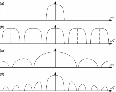
it shows that the interpolated signal is not band-limited. This point is explained schematically in Fig. 2. The term P
mF(ω−mωs) is clearly of infinite extent in the frequency domain; the lack
of aliasing in the sampled signal only guarantees that its components do not overlap one another (Fig. 2(b)). The kernel transformH(ωT) is also not band-limited (Fig. 2(c)). Hence neither is the productFi(ω) (Fig. 2(d)).
One might argue that Fi(ω) can be made effectively band-limited by an appropriate choice
of interpolation scheme. Certainly H(ωT) will decay with increasing frequency, so Fi(ω) will
become negligible at some point. However, this point is inevitably above the Nyquist frequency of the sampled signal, because the interpolation requirements h(−1) = 0, h(0) = 1, h(1) = 0 force the interpolator to contain non-negligible energy at this frequency. Hence any scheme which samples the interpolant at the same rate as the measurement inevitably introduces some degree of aliasing. Furthermore, this problem is notnecessarily solved by over-sampling, which increases the separation of the contributions F(ω−mωs), but does not stop them aliasing back onto the
frequencies of interest. To understand when, and why, it does help, consider again the schematic representation of Fig. 2. The effect of reducing the sample interval T is shown in Fig. 3; the signal transform narrows, while the interpolator transform remains unchanged. Thus over-sampling reduces aliasing contamination only if (as in the case shown) the interpolator transform is lower around multiples of the sampling frequency than it is in general.
There is, however, no particular reason to insist that the interpolant be re-sampled at the same rate as the measurement. Since the interpolant is defined for all possible times, its sampling frequency could, in principle, be arbitrarily high. In practice, it cannot be increased indefinitely, but there is clearly scope for better control of aliasing if it can be chosen independently. Henceforth, this freedom will be assumed.
(a)
(b)
(c)
(d)
Figure 2: Schematic representation of the effect of interpolation on the frequency content of the measured signal: (a) signal Fourier transform,F(ω); (b) signal Fourier transform and its aliases (dashed lines at multiples of sampling frequency); (c) Fourier transform of the interpolator; (d) Fourier transform of the interpolated signal,Fi(ω), formed
from the product of (b) and (c).
(a)
(b)
(c)
(d)
Figure 3: Schematic representation of the effect of interpolation on the frequency content of an over-sampled measured signal. Subplots as Fig. 2.
2.3. Error analysis
The standard measure of error in the interpolated signal is the ‘mean-square’ expression 2 =
Z ∞
−∞
[fi(t)−f(t)]2 dt, (9)
or, equivalently (via Parseval’s theorem), 2 = 1
2π
Z ∞
−∞
|Fi(ω)−F(ω)|2dω. (10)
On substituting Eq. (7), we obtain a summation of band-limited integrals. Each can be shifted so that it refers to the base frequency range containing the measured signal, with the result
2= 1 2π Z ωs/2 −ωs/2 E(ωT)|F(ω)|2dω, (11) where E(v) = [1−H(v)]2+ X m6=0 [H(v+ 2πm)]2. (12)
This expression is given by Park and Schowengerdt [15]; it also arises when the discrete error associated with re-sampling at unchanged frequency is averaged over sample shift [12]. It is attractive because the integrand is proportional to the original signal spectrum, and the con-stant of proportionality E(ωT) depends only on the interpolation scheme. However, it is also potentially misleading, because it effectively aliases the interpolator transform. The actual er-ror at frequency ω is [1−H(ωT)]2|F(ω)|2 for |ω| ≤ ω
s/2, and [H(ωT)]2|F(ω −mωs)|2 for
(m −1/2)ωs ≤ ω ≤ (m+ 1/2)ωs, m 6= 0. If the interpolated signal is suitably sampled and
then Fourier analysed, with attention focussed on the physically relevant range |ω| ≤ ωs/2, the
m6= 0 errors need not be of concern.
A clearer, but less compact, alternative is simply to consider the difference betweenFi(ω) and
F(ω) as a function of frequency, or, equivalently, to compareH(ωT) with its ideal, ‘boxcar’ form:
Hideal(v) = 1, |v| ≤π;
= 0, otherwise. (13)
This is the approach followed by Lehmann et al. [13]. 2.4. Convergence
It is natural to expect that the interpolation error should decrease as the sampling time-step T decreases. More carefully, we can ask how 2 depends on T as T → 0. This question can be addressed by analysing the frequency-domain expression for 2, Eq. (11). For small T, we can expand E(ωT) about the origin as a Taylor series. Note thatE(v) is even in v, so
2π2 =E(0) Z ωs/2 −ωs/2 |F(ω)|2 dω+T2E 00(0) 2! Z ωs/2 −ωs/2 ω2|F(ω)|2 dω+. . . . (14)
Hence, for→0 asT →0 we requireE(0) = 0, and then∼O(T). If we also haveE00(0) = 0, then ∼O(T2), and the convergence is more rapid. This argument clearly generalises: if derivatives of E(v) up to order 2J are zero at v= 0, ∼O(TJ+1) as T →0.
Now consider the implications for the interpolator transform, H(v). The first requires each term in Eq. (12) to be zero whenv= 0 (since all are non-negative). Therefore
H(2πm) = 1, m= 0;
= 0, m=±1,±2, . . . . (15)
The conditions for m 6= 0 are reminiscent of the qualitative requirement for over-sampling to be beneficial (Section 2.2). The link is unsurprising; both viewpoints effectively consider the high-frequency content to be aliased into the Nyquist range, and the T → 0 limit corresponds to ever greater over-sampling.
The analysis required for the higher-order conditions is straightforward but laborious, and is not set out here. It yields a surprisingly simple result; for E and its first J even derivatives to be zero, in addition to Eq. (15) the first J (even and odd) derivatives of H(v) must be zero at v = 2πm (including m = 0). This establishes a direct link between H(v) and the convergence behaviour of the interpolator.
A less abstract condition can now be derived, with the aid of the differentiation formula given in Appendix A.2. The gradient conditions onH(v) imply
Z ∞
−∞
ujh(u)e−i2πmudu= 0, j= 1, . . . , J. (16)
We shall show that this means any monomial function of the form f(t) = tp, with p an integer
between zero andJ, is reproduced exactly by the interpolator. In this instance, the interpolated function is given by
fi(t) = X n (nT)ph t T −n . (17)
As in Section 2.2, we recast this expression as a convolution integral and substitute the Fourier-series representation for the delta-function train to obtain
fi(t) = ∞ X m=−∞ Z ∞ −∞ (uT)ph t T −u ei2πmudu. (18)
The substitutionq =t/T −u gives
fi(t) = X m ei2πmt/T Z ∞ −∞ (t−qT)ph(q)e−i2πmqdq. (19)
The term (t−qT)p can now be expanded, and Eq. (16) employed to show that the only non-zero
contribution comes fromtp. The conditions on H(2πm), Eq. (15), then eliminate all terms in the
summation apart fromm= 0, sofi(t) =tp=f(t), as claimed.
Thus convergence of the form ∼ O(TJ+1) implies that the interpolator is capable of re-producing monomials, and therefore also polynomials, up to order J. The converse applies too; starting from the reproduction property one obtains the convergence result. This can alternatively
be demonstrated directly via the observation that an interpolator with the reproduction property matches the local Taylor series forf(t) up to the term of order TJ. Expanding the terms f(nT)
in Eq. (1) as Taylor series aboutn= 0, and reversing the summation order, we have
fi(t) = J X j=0 f(j)(0) j! X n (nT)jh t T −n +O(TJ+1). (20)
The polynomial-reproduction property implies that the summation over n is simply tj, and the
right-hand side is then recognisable as the Taylor series for f(t) about t = 0. The difference between fi(t) and f(t) is thus O(TJ+1). The Taylor-series-matching property can profitably be
used as a requirement when deriving practical interpolators [11]. 2.5. Regularity
The term ‘regularity’ refers to the degree of continuity of the interpolator, i.e. how many times it can be differentiated before discontinuities are encountered. The linear interpolation kernel of Fig. 1, for example, is continuous in value but discontinuous in its gradient.
In the light of the link between convergence order and Taylor-series matching, one might expect that regularity and convergence are two sides of the same coin. In fact, however, they are distinct properties. For example, the linear interpolation kernel reproduces functions of the formc0+c1t, withc0 and c1 constant, exactly. Hence it matches the first two terms in the Taylor series, but it is only continuous in value. In the special case of a straight line, it produces an interpolated func-tion with a continuous gradient, but in general the interpolant will have gradient discontinuities. Similarly, Keys’ cubic interpolator [11] can reproduce the quadratic c0+c1t+c2t2 and matches the first three terms in the Taylor series, but is only continuous in value and gradient.
Furthermore, not only are regularity and convergence not synonymous, they are not even (de-spite the previous examples) straightforwardly related. Schaum [12] designed polynomial ‘LF’ interpolators subject to the interpolation and reproduction-of-monomials requirements. This ap-proach allows arbitrarily high convergence order to be achieved, but all members of the family have either value or gradient discontinuities.
The disconnect between convergence and regularity arises becauseis a global quantity defined via an integral of the interpolation error, whereas discontinuities are local phenomena. Alterna-tively, in the Fourier domain, the regularity of the interpolator determines the overall decay of H(ω) at high frequencies [16, Ch. 4].1 In contrast, the convergence conditions are linked to local smoothness ofH(ω) at zero frequency, and at multiples of the sampling frequency.
2.6. Support
The term ‘support’ refers to the extent of an interpolator. Considering again the example of Fig. 1, we see that the linear interpolator has support 2. Increasing the support creates greater freedom in interpolator design, allowing regularity and convergence properties to be improved. The chief drawback is numerical cost [14]. The issue of boundary conditions at data start and end points may also be important, if accurate interpolation in these regions is desired.
1
For an accessible analogy, one can inspect the Fourier series coefficients of a square wave and a triangle wave [17, Ch. 10]. The square wave has value discontinuities, and its coefficients decay with ordernliken−1. The triangle wave is continuous, with gradient discontinuities, and its coefficients decay liken−2.
2.7. Stationary random signals
The foregoing theoretical exposition has implicitly assumed that the Fourier transform of the measured signal is well defined. However, in many applications the signal will be stochastic, and the assumption is untenable. It is tempting to claim, by analogy with standard results, that we can translate directly to the stochastic case simply by replacing the signal transform with its spectral density, and the interpolator transform with its square. Indeed, at first sight, this is the claim made by Blu and Unser [18]. Closer examination, however, reveals that they envisage a further averaging step. Hence the issue must be analysed in more detail.
First, note that we can legitimately work with the nominal, infinite-extent, interpolated signal. (The practical, finite-length, version can be seen as the result of truncating the nominal inter-polant, rather than of interpolating the truncated original, as long as edge effects arising from the interpolation are properly eliminated.) Hence we consider the auto-correlation function of the nominal interpolated signal:
fi(t1)fi(t2) = X m,n Rf f[(n−m)T]h(t1/T−m)h(t2/T −n), (21) where Rf f(τ) =f(t)f(t+τ) (22)
is the auto-correlation of the original, stationary, signal. Note there is no guarantee that the interpolated signal is stationary, because its auto-correlation is not necessarily a function of (t2−t1) only. To pursue this question, we investigate the generalised spectrum
Sfifi(t1, ω) =
Z ∞
−∞
fi(t1)fi(t1+τ)e−iωτdτ. (23) On substituting Eq. (21), the integral overτ can immediately be expressed in terms of the inter-polator Fourier transform. The summations are evaluated in the same way as previously (cf., for example, Section 2.2), by expressing them in integral form via delta-function convolutions. The final result is Sfifi(t1, ω) =S (a) f f(ω)H(ωT) X m e−i2πmt1/TH(ωT + 2πm), (24)
where Sf f(a)(ω) is the spectrum of the original signal, Sf f(ω) (the Fourier transform of Rf f(τ)),
repeated at intervals of the sampling frequency: Sf f(a)(ω) =X
m
Sf f(ω+mωs). (25)
This is the expected spectral counterpart of the aliased signal transform that appears in Eq. (7). However, the intuitive suggestion that it should be multiplied by the square of the interpolator transform is clearly wrong. The correct result includes other terms, and also explicitly demonstrates that the interpolated signal is not stationary, since the generalised spectrum is not independent of t1. Instead, it has an oscillating variation with period T.
The need for the additional averaging step is now clear. The mean of Eq. (24) over one period is 1 T Z T /2 −T /2 Sfifi(t1, ω) dt1 =S (a) f f(ω) [H(ωT)] 2, (26)
which is the intuitively expected result. A fundamental justification for performing the average is not, to the author’s knowledge, available. However, Appendix B presents an analysis which provides support for the operation. Once accepted, it implies that the theoretical results discussed in this section carry over without alteration to the stochastic case. Henceforth, this point will be taken as read.
2.8. Choice of interpolator metric
In the final reckoning, both practical and theoretical considerations will determine the best interpolator. Having reviewed the background theory, we are now in a position to discuss the latter, and to specify an appropriate measure of interpolator quality.
In their review of interpolation, Th´evenaz et al. [14] focus on the integral error measure in the form of Eq. (11). On this basis they conclude that regularity is only important if the interpolated function is to be differentiated. However, in the context of acoustic measurements, we expect the underlying signal to be continuous in value and derivatives. Physically, therefore, one might argue that the interpolated signal should mirror this property to the greatest extent possible. We shall reconsider this qualitative requirement, and its quantitative implications, subsequently.
Returning to the error measure, Th´evenaz et al. write the leading-order term of its small-T expansion, Eq. (14), in the form
2= C 2T2J 2π Z ωs/2 −ωs/2 ω2J|F(ω)|2 dω, (27)
and then compare a range of interpolators on the basis of the constantC and the convergence order J. They argue that the convergence order is the most important accuracy parameter, because the T2J term ensures that higher-order interpolators always ‘win’ over lower, irrespective of their C
values, asT →0.
While indisputably true, this point is not directly relevant in the current context. Here our sampling interval will typically be fixed by the bandwidth of the measured signal, and practical constraints will prevent its being lowered beyond a certain point. We wish to identify the best option for a givenT, and it is entirely possible to envisage a lower-order interpolator that performs better by virtue of a small term multiplying T2J. Furthermore, if the sampling is reasonably
efficient, the leading-order estimate for given by Eq. (27) may itself be inaccurate. Essentially, it rests on the value of T being small enough that F(ω) and its shifted images are concentrated around the regions ωT = 2πm, i.e. on progression along the over-sampling route from Fig. 2 to well beyond Fig. 3. In practice, one aims to sample so that F(ω) and its images are much less separated. In this case, approximation of the Fourier transform of the interpolation by expanding H(ωT) aboutωT = 2πm is of dubious legitimacy; the resulting series is unlikely to be dominated by its leading-order term alone.
The assumptionT →0 is not necessary if one considers the exact error. However, its represen-tation in the form of Eqs. (11) and (12) includes the spurious energy at frequencies above Nyquist that is present in the interpolated signal. Once the interpolant and measurement sampling frequen-cies are decoupled, it is better to consider the more fundamental form provided by the integrand of Eq. (10). In this context, the relevant issues are (cf. Eq. (7)): (i) how rapidlyH(v) decays for |v| ≥ π (so that re-sampling requirements are not excessive); and (ii) how close to unity H(v) is for|v|< π (so that the original signal is recovered without attenuation).
In the light of this discussion, it is necessary to revisit the convergence conditions, Eq. (15) and H(j)(2πm) = 0 forminteger (withj < J, the convergence order). At first sight, it seems that they are no longer relevant. However, the zero-frequency requirements can alternatively be interpreted as increasing ‘flatness’ constraints onH(v) at low frequencies, which will keep it as close as possible to its ideal value in the range likely to be of most interest. (This point was the rationale behind Schaum’s ‘LF’ interpolator designs [12]. Note also that the odd derivatives are identically zero by virtue of symmetry.)
Outside the Nyquist range, the discrete conditions on H(v) at v = 2πm are replaced by the more general condition that H(v) should decay to negligible levels as fast as possible. Here the issue of regularity re-enters. Since greater regularity implies more rapid high-frequency decay, the intuitive physical requirement mooted at the beginning of this section has a potential impact on re-sampling frequency. However, it need not be included as a separate criterion, as its influence is implicit inH(v).
3. Candidate interpolators
The previous section identified a suitable performance measure for an interpolator h(u): its Fourier transform H(v), as defined by Eq. (8). In this part of the paper, we assess specific in-terpolators on the basis of their Fourier transforms. First, in Section 3.1, we introduce the three families that will be considered. Then their parametric dependence is characterised in Section 3.2. For each family, a preferred sub-set is identified for subsequent, inter-family, comparison.
3.1. Types of interpolator
The material in this section is based on the surveys of Lehmann et al. [13] and Th´evenaz et al. [14]. Only the promising candidates from these references are considered.
3.1.1. Piecewise-polynomial interpolators
Piecewise-polynomial interpolators are constructed from concatenated polynomial segments usually, but not necessarily, joined at integer values of the interpolator argument u. They are straightforward to generate, and allow great freedom in design. They are also cheap to evaluate numerically. Many different versions are documented in references [13] and [14].
3.1.2. Sinc-based interpolators
The ideal interpolator is the ‘sinc’ function:
sinc(u) = sinπu
πu . (28)
This result follows straightforwardly from inverse Fourier transformation of the ideal frequency-domain form, Eq. (13). It is informative, but of little practical use because sinc(u) is of infinite extent. Although a truncated sinc still satisfies the interpolator conditions, Eq. (3), it has poor frequency-domain properties [13, 14]. Improvements are possible, however, if the sinc is ‘windowed’; in particular Lehmann et al. [13] include a ‘DC-constant’ form which performs well in their tests. They do not recommend it, however, because of numerical costs.
3.1.3. Interpolators derived from basis functions
Rather than starting from the explicit representation of Eq. (1), one can instead specify that the interpolant should be formed from a superposition of scaled and shifted instances of a basis function, φ(u). This has the advantage that basis functions with desirable properties can be specified, but the disadvantage that the underlying interpolator is not known explicitly. Instead, it is necessary to revert to the original interpolation condition: sample values should be reproduced exactly. Thus, if
fi(t) = X
k
ckφ(t/T−k), (29)
withck the set of scaling coefficients, then
fi(nT) = X
k
ckφ(n−k) =f(nT), (30)
and this requirement allows theckto be determined. The matrix-inversion nature of the calculation
implies that all samples influence each coefficient; equivalently, the underlying interpolator is infi-nite in extent. Although this might suggest that the approach is impractical, efficient and effective numerical techniques exist when the basis functions are the so-called ‘B-splines’ [14]. Th´evenaz et al. [14] strongly recommend B-spline interpolation; Lehmann et al. [13] also regard it as gen-erally advantageous, but with a reservation over ‘edge effects’ at the beginning and end of the measurement sequence.
3.2. Interpolator characteristics 3.2.1. Linear interpolation
To provide a baseline for subsequent results, we first consider the transformH(v) of the linear interpolator defined by Eq. (2). It is calculated using the general piecewise-polynomial formulation, as described in Appendix C.2. Figure 4 shows the result, plotted on a decibel scale. In the light of Eq. (7), the Nyquist frequency of the measured signal is at v/π = 1. The level here is around −8dB. Over-sampling by a factor of 2 corresponds to a signal band-limited to|v|/π <0.5, in which case the potential aliasing (if the interpolated signal is sampled at the same rate) is most severe from components atv/π = 1.5. These arise from the signal content at v/π = 0.5, attenuated by only 20dB. On a linear measure, this represents a spurious contribution of 10%.
Although of concern, the aliasing issue can always be handled, as the interpolated signal can be re-sampled arbitrarily fast. However, attenuation of components below Nyquist is a greater worry, as this cannot be reversed. (Recall that de-Dopplerisation alters frequencies, so the spectrum of the source-time signal cannot simply be corrected by the known modification of the receiver-time spectrum.) Figure 5 shows the error, 1−H(v), over 80% of the original signal’s Nyquist range. It becomes significant very quickly, exceeding 10% after v/π = 0.36. Clearly, components at frequencies approaching Nyquist in the sampled signal will be unacceptably degraded. However, even those atv/π= 0.5 are attenuated by 19%, or 1.8dB. This ‘in-bound’ error was not considered by Howell et al. [2] when they recommended two-times over-sampling. Note also that any aliasing error can only add to it, as is evident from Eq. (12).
0 1 2 3 4 5 -120 -100 -80 -60 -40 -20 0
Figure 4: Fourier-transform magnitude for the linear interpolator of Eq. (2). The vertical dashed line is at the Nyquist frequency of the sampled signal.
0 0.1 0.2 0.3 0.4 0.5 0.6 0.7 0.8 0 0.05 0.1 0.15 0.2 0.25 0.3 0.35 0.4
3.2.2. Piecewise-polynomial interpolators
Given the interpolation conditions, it is natural (although not essential) to join the polynomial pieces at integer arguments. Hence we formulate the general interpolator of orderK and support 2N as h(u) = K X k=0 bn,k|u|k n−1≤ |u|< n, n= 1,2, ..., N; = 0. N ≤ |u|. (31)
where the bn,k are coefficients to be determined. They are specified by imposing requirements
on the interpolator. In particular, it is constrained to have value and derivative continuity up to degreeK−2 (so, for example, a cubic will have continuous gradient but discontinuous curvature). It is also required to have unity gain at DC, i.e.H(0) = 1. Then any remaining degrees of freedom are used to increase the low-frequency flatness of H(v) by settingH(2J)(0) = 0 for J = 1, 2, etc. (The odd derivatives are identically zero by symmetry.) Details of the derivations are given in Appendix C.1.
Table 1 summarises the piecewise polynomials with 2≤N ≤4 and 2≤K≤7 that follow from this approach. AsN increases, the maximum possible polynomial order also increases. For a given value ofN, higher polynomial order (and hence degree of continuity) comes at the price of reduced low-frequency flatness. Alternatively, for fixed order, greater low-frequency flatness is attainable with greater extent. The instances (N, K) = (2,3), (3,5) and (4,7) correspond to Meijering et al.’s interpolators [19]. Of these, the first is Keys’ cubic [11].
Table 1: Degree of low-frequency flatness, 2J inH(2J)(0) = 0, achieved for piecewise polynomials of degreeK and support 2N. All have derivative continuity up to degreeK−2 and DC gainH(0) = 1. Crosses indicate unachievable cases. N K 2 3 4 5 6 7 2 2 2 0 0 × × 3 4 4 2 2 0 0 4 6 6 4 4 2 2
The interpolator transforms could be estimated numerically, but this would introduce the poten-tial for error in low-amplitude regions. Hence here, and for subsequent types, analytical expressions are derived and evaluated. For the piecewise polynomials, the analysis is presented in Appendix C.2.
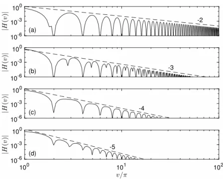
First, the theoretical influence of continuity degree on the high-frequency decay ofH(v) (cf. Sec-tion 2.5) can be confirmed by considering interpolators of different polynomial order. Figure 6 shows the N = 2 results, plotted on logarithmic scales. The theoretical dependence implies that H(v) should roll off like vK (e.g. for K = 2, the interpolator is continuous in value but not gradient,
and this leads to second-order decay). This behaviour is clearly evident in Fig. 6. The figure also demonstrates that 40dB attenuation at frequencies not far in excess of Nyquist is possible if one employs interpolators of higher order than quadratic. This implies that re-sampling requirements
could be relatively benign, in which case high-frequency decay characteristics would not be im-portant (because aliasing errors would be dominated by contributions from frequencies below the roll-off region). As similar features are found for N = 3 and 4 as well, only cubic and higher polynomials will henceforth be considered.
10-6 10-3 100 (a) -2 10-6 10-3 100 (b) -3 10-6 10-3 100 (c) -4 100 101 102 10-6 10-3 100 (d) -5
Figure 6: Fourier-transform magnitude for piecewise-polynomial interpolators withN = 2: (a)K= 2 (quadratic); (b)K= 3 (cubic); (c)K= 4 (quartic); (d)K= 5 (quintic).
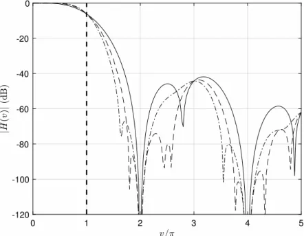
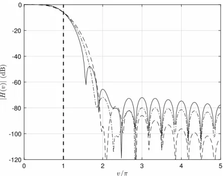
Figure 7 shows the frequency content of the N = 3 interpolators from cubic to septimic. It confirms more clearly the 40dB attenuation claim and shows that this value is achieved within the main lobe. It also shows rather similar levels in the initial side lobe(s), between v/π = 2 and v/π = 4, irrespective of polynomial order. This has a significant implication: if aliasing errors of this magnitude are tolerable, the improvement in continuity degree associated with higher orders is irrelevant. Indeed, stronger continuity is actually detrimental in terms of the 40dB cut-off frequency, which increases from approximately 1.6 to 1.9 times Nyquist between the cubic and septimic.
Turning to the error in the sub-Nyquist range containing the measured signal, Fig. 8 shows that the cubic interpolator is again superior. This is straightforwardly explainable in terms of the low-frequency conditions imposed on the associated transform, whose first five derivatives are all zero at v = 0. Its error at v/π = 0.5 is 2.6%, compared to 11.6% for the septimic (and 19% for linear interpolation; note the altered scale compared to Fig. 5).
The cubic is similarly superior to higher orders for interpolators withN = 2 andN = 4. Hence it remains only to characterise the influence ofN on the cubic interpolators. The results forK = 3 and N = 2 to 4 are presented in Figs. 9 and 10. They show that increasing N is beneficial for accuracy; both the 40dB cut-off frequency and the sub-Nyquist error are reduced. Revisiting the hypothetical example in which the signal spectrum is in the lower half of the sub-Nyquist band (two-times over-sampling) and the interpolated signal is sampled at the same rate, withN = 4 we
0 1 2 3 4 5 -120 -100 -80 -60 -40 -20 0
Figure 7: Fourier-transform magnitude for piecewise-polynomial interpolators withN= 3: —, K= 3; – –,K= 4; –·–,K= 5;· · ·,K= 6; ,K= 7. The vertical dashed line is at the Nyquist frequency of the sampled signal.
0 0.1 0.2 0.3 0.4 0.5 0.6 0.7 0.8 0 0.02 0.04 0.06 0.08 0.1 0.12 0.14 0.16 0.18 0.2
Figure 8: Relative error in the piecewise-polynomial-interpolated signal at frequencies below Nyquist: —, K= 3; – –,K= 4; –·–,K= 5;· · ·,K= 6; ,K= 7. Semi-supportN = 3 in all cases.
have worst-case aliasing components 40dB down (compared to 20dB for linear interpolation), and attenuation error 1.2%, or−0.1dB (compared to−1.8dB).
0 1 2 3 4 5 -120 -100 -80 -60 -40 -20 0
Figure 9: Fourier-transform magnitude for piecewise-polynomial interpolators withK= 3: —,N = 2; – –,N = 3; –·–,N= 4. The vertical dashed line is at the Nyquist frequency of the sampled signal.
3.2.3. Sinc-based interpolators
The ‘windowed’ sinc functions discounted by Th´evenaz et al. [14] have clearly sub-optimal windows. With a better choice, it is possible to achieve good properties [13]. Thus, in spite of the recognised numerical cost issues, it is still worth considering this type.
The interpolator is written in the form
h(u) =w(u) sinc(u), (32)
where w(u) is a finite window function of length 2N. Following Lehmann et al. [13], we consider the three-term form
w(u) =a0+a1cos πu N +a2cos 2πu N . (33)
For a2 = 0, the classic Hann window is regained by setting a0 =a1 = 0.5. However, as noted by Th´evenaz et al., the resulting interpolator fails to satisfy the DC-gain requirement, H(0) = 1. It is, however, straightforward to find an alternative pair (a0, a1) that still generate an interpolator (a0+a1 = 1) while yielding H(0) = 1 (Appendix D.1). Their values vary with N; the associated two-term window differs from that of Hann in being discontinuous at u = N. The interpolator itself is continuous, by virtue of sinc(N) = 0.
When the third term is introduced, an additional condition can be imposed. This is used either to improve low-frequency behaviour, or degree of continuity. In the former case,a2is chosen so that H00(0) = 0; in the latter so that w(N) = 0. Note that, since w0(N) = 0 identically, this improves
0 0.1 0.2 0.3 0.4 0.5 0.6 0.7 0.8 0 0.02 0.04 0.06 0.08 0.1 0.12 0.14 0.16 0.18 0.2
Figure 10: Relative error in the piecewise-polynomial-interpolated signal at frequencies below Nyquist: —,N = 2; – –,N= 3; –·–,N = 4. OrderK= 3 in all cases.
regularity by two levels, i.e. h00(u) is now continuous. The derivations for these ‘low-frequency’ and ‘improved-regularity’ windowed-sinc interpolators are given in Appendix D.1.
Appendix D.2 describes the analysis required to obtain the interpolator Fourier transforms. Figure 11 shows the upshot forN = 3. Broadly speaking, the features are as expected in the light of the piecewise-polynomial results: improved regularity leads to more rapid decay at high frequencies, but a higher main-lobe cut-off frequency. However, there are important detail differences. First, the overall side-lobe levels are much lower than for polynomials. Also, the anticipated v−2 decay for the interpolators with value continuity only (two-term and low-frequency) only starts to appear towards the upper frequencies in the plotting range. Finally, for main-lobe cut-off levels up to almost 50dB, the two-term window has the lowest cut-off frequency, thanks to a local minimum that is not present for the three-term windows.
The sub-Nyquist error also exhibits an unexpected feature, as shown in Fig. 12. Although the low-frequency three-term window is superior to its more regular counterpart, the two-term window has the most delayed growth. On closer examination, this is seen to be due to a ‘ripple’ at lower frequencies (hence the need to plot|1−H(v)|instead of 1−H(v)). The peak error associated with the ripple is 0.3% in the region ofv/π= 0.33
If the interpolator size is increased to N = 4, the qualitative features described above remain unchanged and performance of the interpolators improves. When it is decreased toN = 2, however, the anomalous local minimum and the sub-Nyquist ripple associated with the two-term window disappear, and the three-term low-frequency window is unambiguously superior.
3.2.4. B-spline-based interpolators
For comparability, we will consider interpolators arising from B-splines with extent 2N. The associated polynomials are then of order 2N−1, and the basis functions are continuous up to and
0 1 2 3 4 5 -120 -100 -80 -60 -40 -20 0
Figure 11: Fourier-transform magnitude for windowed-sinc interpolators withN = 3: —, two-term; – –, improved-regularity; –·–, low-frequency. The vertical dashed line is at the Nyquist frequency of the sampled signal.
0 0.1 0.2 0.3 0.4 0.5 0.6 0.7 0.8 0 0.02 0.04 0.06 0.08 0.1 0.12 0.14 0.16 0.18 0.2
Figure 12: Relative error in the windowed-sinc-interpolated signal at frequencies below Nyquist: —, two-term; – –, improved-regularity; –·–, low-frequency. Semi-supportN= 3 in all cases.
including derivative 2N −2 [20]. By construction, therefore, the associated interpolator inherits these properties. Appendix E describes how the interpolators and their Fourier transforms can be calculated.
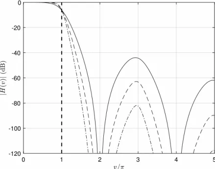
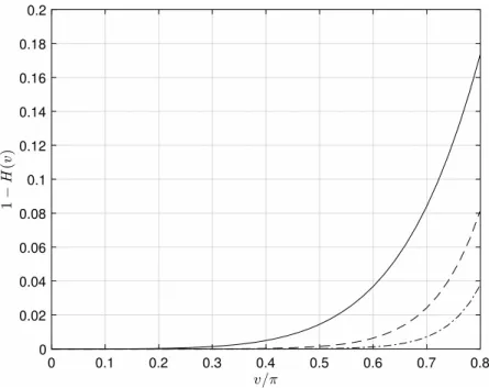
Figure 13 plots the frequency context of the interpolators derived from the B-splines with N = 2, 3 and 4 (orders 3, 5 and 7). There is a clear trend towards lower main-lobe cut-off frequency and reduced sidelobes as N increases. Likewise, the error properties at sub-Nyquist frequencies (Fig. 14) also improve with N. Indeed, all three interpolators show exemplary low-frequency flatness, despite the absence of any explicit condition on this property, and the 7th-order instance maintains better than 1% accuracy up to frequencies in excess of 0.7 times Nyquist.
0 1 2 3 4 5 -120 -100 -80 -60 -40 -20 0
Figure 13: Fourier-transform magnitude for B-spline-based interpolators: —,N= 2; – –,N = 3; –·–,N= 4. The vertical dashed line is at the Nyquist frequency of the sampled signal.
3.3. Summary
In this section, we have investigated the parametric dependence of piecewise-polynomial, windowed-sinc, and B-spline-based interpolators. All the options exhibit markedly better accuracy than linear interpolation. Each type benefits from an increase in its extent (support). In the piecewise-polynomial family, there is unlikely to be any practical benefit associated with increasing regularity beyond the gradient continuity afforded by the cubic members. The optimum windowed-sinc in-terpolator depends on extent. For N = 2 (support 4), a three-term window enforcing H00(v) = 0 in addition to the DC-gain condition performs best. ForN = 3 and 4, a two-term window satisfy-ing the DC-gain condition only is preferable (assumsatisfy-ing that low-frequency ripple below the error tolerance is acceptable). Finally, the B-spline-based interpolator is uniquely determined for each value of N.
0 0.1 0.2 0.3 0.4 0.5 0.6 0.7 0.8 0 0.02 0.04 0.06 0.08 0.1 0.12 0.14 0.16 0.18 0.2
Figure 14: Relative error in the B-spline-based interpolated signal at frequencies below Nyquist: —, N = 2; – –,
N= 3; –·–,N = 4.
4. Discussion and recommendations
The previous part of the paper considered three types of interpolator — piecewise-polynomial, windowed-sinc, and B-spline-based — and identified, for a given extent (‘support’) the best in-stances of each. The next question is how they compare against one another. This issue is ad-dressed in Section 4.1. The results are then discussed in Section 4.2, in terms of both accuracy and other considerations. Finally, Section 4.3 explores the practical implications by presenting recommendations for a specific accuracy-requirement scenario.
4.1. Comparison of interpolator types
Figure 15 shows the frequency contents of the support-4 (semi-support N = 2) cases. The cubic piecewise polynomial and the windowed sinc are almost indistinguishable over most of the main lobe, but the latter has lower initial side-lobe levels. The B-spline-based interpolator has a main lobe closer to the pass-stop ideal, and initial side-lobe level comparable to the piecewise polynomial.
Figure 16 shows the comparison at sub-Nyquist frequencies in more detail. The close match be-tween the piecewise-polynomial and windowed-sinc interpolators continues down to zero frequency, and the superiority of the B-spline formulation in this region is confirmed.
Increasing the semi-support to N = 3 (Fig. 17), one finds bigger differences between the opti-mum windowed-sinc interpolator (now using the two-term window) and the piecewise-polynomial. This is due to the change in window formulation; the comparison with the low-frequency windowed-sinc form for N = 3 (not shown) exhibits the same features as for N = 2. The upshot is that, in addition to having lower initial sidelobe levels, the windowed-sinc interpolator has a slightly faster main-lobe decay down to the first minimum. The B-spline-based interpolator again appears
0 1 2 3 4 5 -120 -100 -80 -60 -40 -20 0
Figure 15: Fourier-transform magnitude for interpolators withN = 2: —, cubic piecewise polynomial; – –, low-frequency windowed sinc; –·–, B-spline-based. The vertical dashed line is at the Nyquist frequency of the sampled signal. 0 0.1 0.2 0.3 0.4 0.5 0.6 0.7 0.8 0 0.02 0.04 0.06 0.08 0.1 0.12 0.14 0.16 0.18 0.2
Figure 16: Relative error in the interpolated signal at frequencies below Nyquist: —, cubic piecewise polynomial; – –, low-frequency windowed sinc; –·–, B-spline-based. Semi-support N = 2 in all cases. Note the overlay of the polynomial and windowed-sinc curves.
superior in all aspects except for initial side-lobe level (compared to the windowed sinc); note, however, that the difference is smaller than for N = 2, and the absolute value is now below the first windowed-sinc maximum (approximately−50dB).
0 1 2 3 4 5 -120 -100 -80 -60 -40 -20 0
Figure 17: Fourier-transform magnitude for interpolators withN = 3: —, cubic piecewise polynomial; – –, two-term windowed sinc; –·–, B-spline-based. The vertical dashed line is at the Nyquist frequency of the sampled signal.
The detail error plot (Fig. 18) shows that the difference between the piecewise polynomial and the windowed sinc persists well into the sub-Nyquist band. Only below one-third Nyquist is the polynomial better, and here the error in both lies comfortably below 0.5%. Meanwhile, the superiority of the B-spline formulation is again confirmed.
Finally, the comparison plots forN = 4 (Figs. 19 and 20) exhibit the same qualitative features as those for N = 3, but are included as a basis for the quantitative recommendations to follow. There is one key difference, however: the B-spline formulation is now unambiguously superior, because its sidelobes never rise above those of the windowed sinc.
4.2. Discussion
In terms of accuracy alone, the results presented here provide ample support for Th´evenaz et al.’s conclusion in favour of B-splines [14]. Recall that there are two concerns: sub-Nyquist error due to main-lobe attenuation; and out-of-band error due to side-lobe multiplication of the additional frequencies introduced by the original sampling. The former determines how much of the nominal signal range is usable, and the latter dictates the re-sampling frequency needed to avoid unacceptable aliasing in this region. Although it is possible to conceive of a combination of aliasing and sub-Nyquist error limits that might favour the windowed sinc forN = 2, this exercise is much harder forN = 3, and impossible for N = 4. Hence, all other factors being equal, B-spline-based interpolation should be employed.
The most obvious extraneous issue is numerical cost. Here, the B-spline formulation apparently suffers relative to the piecewise-polynomial, because the associated interpolator is implicit, and
0 0.1 0.2 0.3 0.4 0.5 0.6 0.7 0.8 0 0.02 0.04 0.06 0.08 0.1 0.12 0.14 0.16 0.18 0.2
Figure 18: Relative error in the interpolated signal at frequencies below Nyquist: —, cubic piecewise polynomial; – –, two-term windowed sinc; –·–, B-spline-based. Semi-supportN = 3 in all cases. Note that windowed sinc has
H(v)>1 forv/π <0.42. 0 1 2 3 4 5 -120 -100 -80 -60 -40 -20 0
Figure 19: Fourier-transform magnitude for interpolators withN = 4: —, cubic piecewise polynomial; – –, two-term windowed sinc; –·–, B-spline-based. The vertical dashed line is at the Nyquist frequency of the sampled signal.
0 0.1 0.2 0.3 0.4 0.5 0.6 0.7 0.8 0 0.02 0.04 0.06 0.08 0.1 0.12 0.14 0.16 0.18 0.2
Figure 20: Relative error in the interpolated signal at frequencies below Nyquist: —, cubic piecewise polynomial; – –, two-term windowed sinc; –·–, B-spline-based. Semi-supportN = 4 in all cases. Note that windowed sinc has
H(v)>1 forv/π <0.58.
is effectively calculated continuously during the interpolation process. However, it is possible to implement the calculation efficiently [21] and the cost overhead is then not significant [14]. Piecewise-polynomial and B-spline-based interpolators thus have comparable costs, and both are cheaper than windowed-sinc, because the latter’s trigonometric functions are expensive to evaluate. Not considered in this argument is the cost of algorithm implementation. Here, the piecewise-polynomial and windowed-sinc options are clearly preferable, as they require only a straightforward transcription of Eq. (1). In contrast, the efficient implementation of B-spline-based interpolation requires a pre-filtering step, which derives the coefficients ck in Eq. (29). The underlying filter
is acausal, so must first be decomposed into causal and anti-causal components, which are then applied forwards and backwards respectively. While not intrinsically difficult, this does represent an obstacle to a first-time user of the method.
A further uncertainty concerns edge effects. The equations defining the coefficientsckin terms
of the measured signal values are coupled, so in principle a given coefficient is influenced by all the measurements. Hence the interpolated signal value is similarly dependent; i.e., as noted previously, the underlying interpolator is of infinite extent. In practice, of course, it decays to a level below which it can be ignored, but the choice of level, and the point at which the interpolator reaches it, must be determined by the user. Fortunately, the behaviour is extremely benign. Figure 21 shows the magnitude of the underlying interpolator forN = 2, plotted on a logarithmic scale. The decay is exponential, and sufficiently rapid that |h(u)| is below 10−6 by |u| = 10. Therefore the only serious additional requirement associated with B-spline-based interpolation is implementation of the pre-filtering stage.
-20 -15 -10 -5 0 5 10 15 20 10-12 10-10 10-8 10-6 10-4 10-2 100
Figure 21: Magnitude of the interpolator derived from the B-spline withN= 2.
4.3. Recommendations
In order to make concrete recommendations, specific error targets are needed. Such targets are, inevitably, arbitrary to some extent. Here, we shall consider a ‘reasonable’ specification with accuracy requirements that would be normal for standard acoustic measurements. Readers with alternative preferences will be able to generate their own analysis parameters using the material presented in this paper.
A reasonable choice for acceptable practical accuracy is to require that aliasing errors are 40dB below the true signal, and that the latter is attenuated by no more than 0.5dB in the range of interest. In percentage terms, this sets aliasing error below 1% and attenuation error below 5.6%. In the light of the previous discussion, recommendations will be given separately for B-spline-based interpolation and for alternatives. The latter are only intended for users unable, or unwilling, to implement the B-spline formulation (in its efficient incarnation). If this formulation is available, the alternative is not recommended.
4.3.1. B-spline-based interpolators
Table 2 shows the recommended analysis parameters and achievable range, given the nominal accuracy specification. The achievable range is simply the frequency value at which the interpo-lator’s frequency-content plot reaches the attenuation error limit (−0.5dB in this case). If this is denotedfa, and the re-sampling Nyquist frequencyfr, then the lowest frequency at which content
that aliases into the achievable range is encountered isfr+ (fr−fa). Choosing this to be the 40dB
cut-off value fixesfr, which is tabulated in the final column. Note that frequencies are quoted as
proportions of the original Nyquist value (corresponding tov/π in the foregoing plots).
The immediate conclusion is that the B-spline-based interpolation can, in principle, allow almost the entire sub-Nyquist range to be measured with reasonable accuracy. Given that even standard
Table 2: Analysis parameters to achieve the nominal accuracy specification with B-spline-based interpolation. Values given are frequencies normalised by the Nyquist value for the measurement.
Semi-support (N) Achievable range 40dB cut-off Re-sampling Nyquist frequency
2 0.65 1.52 1.09
3 0.77 1.37 1.07
4 0.83 1.28 1.06
measurements cannot attain the full range, it appears possible to avoid interpolation-imposed over-sampling entirely. A caveat should be noted, however: the re-sampling frequency might be constrained to match the original, in which case (for these accuracy requirements) the achievable range is set by the 40dB cut-off value. (For example, with N = 3 one would only have alias errors more than 40dB down below 0.63 times Nyquist.) Nonetheless, the need for over-sampling is significantly smaller than previously thought.
The implications of alternative accuracy specifications can straightforwardly be obtained in the same way, with the aid of Figs. 13 and 14. The only potential complication arises if the aliasing error requirement drops below the first sidelobe peak. In principle, one could specify a cut-off frequency on the down-slope of the sidelobe, but this would entail a significant increase in the re-sampling frequency (with an associated numerical cost). Hence, it is recommended that the interpolator in question is simply discarded. Thus, for example, an aliasing-error requirement of −60dB would rule out theN = 2 (cubic) B-spline, and leaveN = 3 orN = 4 as the viable options. 4.3.2. Alternative interpolators
Here the options are the cubic piecewise polynomial and the windowed sinc. An important consideration is the latter’s higher numerical cost. Hence, forN = 2 the choice is straightforward: piecewise polynomial (cf. Figs. 15 and 16). For N = 3 and 4, the windowed sinc offers a slight performance benefit, and the decision becomes less clear. Here, greater weighting is given to the numerical cost, meaning that the recommendation is unchanged. The analysis parameters in this case are summarised in Table 3.
Table 3: Analysis parameters to achieve the nominal accuracy specification with the recommended alternative to B-spline-based interpolation: cubic piecewise-polynomial. Values given are frequencies normalised by the Nyquist value for the measurement.
Semi-support (N) Achievable range 40dB cut-off Re-sampling Nyquist frequency
2 0.49 1.71 1.10
3 0.58 1.57 1.08
4 0.64 1.49 1.07
Turning to possible alternative accuracy specifications, there is again an issue once the aliasing-error requirement reaches the sidelobe level. Unlike the B-spline case, however, the solution is not simply a restriction to higher values of N, because here the initial sidelobe peaks do not diminish significantly with increased interpolator extent. One possibility is simply to increase the cut-off frequency as necessary, and accept much more stringent re-sampling requirements. If this approach
is countenanced, however, the higher-order piecewise polynomials discussed in Section 3.2.2 should also be considered, and the optimum solution will depend on acceptable levels of over- and re-sampling in the specific context. At this stage, it may well be preferable to reconsider accepting the implementation cost of the B-spline approach.
If B-spline-based interpolation remains out of the question, a windowed-sinc interpolator might be the best choice, because the low initial sidelobe levels would allow higher accuracy to be achieved at significantly smaller re-sampling rates. In turn, this would offset the numerical cost penalty as-sociated with trigonometric function evaluations. Should this path be taken, the two-term window withN = 3 or 4 is suggested.
4.4. Summary
We have already noted that B-splines give the best interpolation accuracy for a given support (function extent), and have only a small cost penalty compared to piecewise polynomials. It should also now be clear that they are the most straightforward choice in terms of defining analysis param-eters for accuracy requirements more stringent than those considered here. Their only drawback is an initial implementation cost associated with a more complex formulation than the standard interpolation equation. General guidelines for their application are given in Appendix E.3.
If B-splines are not employed, piecewise-cubic interpolators are the next best option. These can achieve arbitrarily small signal attenuation, given sufficient over-sampling, and aliasing errors below 1% with re-sampling frequencies comparable to the original rate. Coefficients for these interpolators are given in Appendix C.3.
Should an aliasing error limit significantly more stringent than 1% be desired, there is no clear single best alternative to B-splines, and all options will be more expensive numerically. In this instance, two-term-windowed sinc functions with semi-support N = 3 or 4 may be preferable to piecewise polynomials. Expressions for the windows are given in Appendix D.3.
5. Conclusions
This paper has discussed the problem of interpolation from a uniformly spaced set of signal samples, with the specific application of acoustic de-Dopplerisation in mind. First, background theory developed largely in the field of image processing has been summarised and assessed; on this basis it has been argued that the best metric for an interpolator’s performance is its Fourier transform, examined both below and above the Nyquist frequency of the measurement. Then, a selection of promising interpolator types — piecewise-polynomial, windowed-sinc, and B-spline-based — has been examined. Finally, the best instances of each type have been compared against one another, and specific recommendations for practitioners have been set out.
The contributions to acoustic de-Dopplerisation are three-fold. First, the widely accepted accuracy analysis for linear interpolation [2] has been shown to be incomplete; it considers aliasing errors, but not in-band signal attenuation. Second, the possibility of sampling the interpolated signal at a rate different from the measurement has been introduced. The additional flexibility gained thereby allows more efficient bandwidth utilisation for a given set of accuracy requirements. Third, straightforward guidance for choosing interpolators other than linear has been provided.
The main recommendation is the use of B-spline-based interpolators. Although they require an additional, pre-filtering, calculation (because the B-spline basis functions are not themselves inter-polating), they offer the best combination of numerical efficiency and accuracy. Their properties improve with their extent and order; practical options are cubic, quintic and septimic.
A subsidiary recommendation applies if the more complicated B-spline formulation is to be avoided, and aliasing errors up to 1% can be tolerated. In this case, the piecewise-cubic family introduced in Section 3.2.2 should be used. Again, their properties improve with extent. The shortest member corresponds to Keys’ cubic interpolator [11]; the others appear to be novel.
It should be emphasised that even the shortest of these sub-optimal interpolators represents a marked improvement on linear interpolation. If its output is re-sampled at 1.1 times the original rate, it delivers aliasing errors below 1% and attenuation errors below 0.5dB over frequencies up to half (original) Nyquist. In contrast, for the same parameters, linear interpolation gives aliasing errors up to 2.7% and attenuation errors up to 1.8dB.
An aliasing error limit below 1% without using B-splines is achievable, but cost penalties are likely to be high, and no definitive interpolator recommendation is possible. A tentative suggestion is a windowed sinc function, using a two-term window chosen to satisfy the requirement of unity DC gain.
Finally, the reader should be reminded that all frequencies referred to here are in the receiver frame of reference. The usable frequency range in the interpolated source signal will thus be lower than the values quoted here, by the (application-dependent) Doppler shift. This issue, however, applies equally to all interpolators, and hence does not affect the conclusions of the paper.
Acknowledgements
This work was undertaken without external funding. The implicit financial support provided by the University of Cambridge is gratefully acknowledged. Supporting research data are available at: https://doi.org/10.17863/CAM.18617.
Appendix A. Useful mathematical results
Appendix A.1. Fourier-series representation of delta-function train The infinite train of delta functions P
nδ(u−n) is periodic in u, with period unity. Hence it
can be expressed as a Fourier series with base (radian) frequency 2π. Application of the standard formula for the Fourier-series coefficients then yields
∞ X n=−∞ δ(u−n) = ∞ X m=−∞ ei2πmu. (A.1)
Appendix A.2. Inverse Fourier differentiation formula
The result for the Fourier transform of a derivative needs no introduction. Its inverse, how-ever, is less familiar (despite being formally identical). Consider the inverse transform of the kth derivative ofH(v): 1 2π Z ∞ −∞ H(k)(v)eivudv= (−iu) k 2π Z ∞ −∞ H(v)eivudv, (A.2)
the right-hand side following from integration by parts. Hence we see that the inverse transform ofH(k)(v) is (−iu)kh(u) or, equivalently,
Z ∞
−∞
Appendix B. Spectral analysis of the stochastic interpolated function
In Section 2.7, it was shown that the interpolated function of a stationary, random signal is not itself stationary. Here we consider the implications of this result for its spectral analysis.
The finite-length sample of the interpolated function is first written as a window w(t) multi-plying the infinite-extent signalfi(t):
fi(w)(t) =w(t)fi(t). (B.1)
Conventionally, the next step is to average instances of |Fi(w)(ω)|2, where F(w)
i (ω) is the Fourier
transform offi(w)(t). The resulting quantity can be expressed in terms of the generalised spectrum defined in Eq. (23), and the Fourier transform of w(t),W(ω):
F (w) i (ω) 2 = 1 2π Z ∞ −∞ Z ∞ −∞ Sfifi(t1, ω0)W(ω−ω0)w(t1)e i(ω−ω0)t1dt 1dω0. (B.2) NowSfifi(t1, ω0) is a periodic function of t1, so it can be expressed as a Fourier series:
Sfifi(t1, ω0) =
∞
X
n=−∞
sn(ω0)ei2πnt1/T. (B.3)
Substituting this form and performing the integration overt1, we obtain
F (w) i (ω) 2 = ∞ X n=−∞ 1 2π Z ∞ −∞ sn(ω0)W(ω−ω0)W∗(ω−ω0+nωs) dω0, (B.4)
withωs, as previously, the sampling frequency, 2π/T. At this stage, we observe that any properly
chosen window function has W(ω) strongly concentrated around the origin. Therefore the only member of the summation in which there is significant overlap between W(ω−ω0) andW∗(ω− ω0+nωs) is the one with n= 0; all the others have negligible integrands. Thus, to an excellent
approximation, F (w) i (ω) 2 = 1 2π Z ∞ −∞ s0(ω0)|W(ω−ω0)|2 dω0, (B.5) which is the standard result for a signal with spectrum s0(ω0). In our case, this spectrum is given by the formula for the zeroth Fourier-series coefficient, i.e.
s0(ω0) = 1 T Z T /2 −T /2 Sfifi(t1, ω0) dt1. (B.6)
Hence a standard spectral analysis applied to the interpolated stochastic signal will yield a spectrum estimate that is the mean of the generalised spectrum, which justifies the use of this quantity for assessing interpolator performance.
Some limitations of this argument should be acknowledged. First, we have not addressed the impact of the Doppler shift; the analysis remains in terms of receiver time. Second, we have not considered sampling effects. These would clearly be problematic if the sampling rate were identical to the original and with a fixed offset throughout. However, de-Dopplerisation will produce varying offsets, and our final recommendations include altered sampling rates. In this context, averaging of the underlying generalised spectrum is to be expected, and the analysis presented here thus carries weight.