North American extreme temperature events and related large scale meteorological patterns: a review of statistical methods, dynamics, modeling, and trends

2-2016

North American extreme temperature events and

related large scale meteorological patterns: a review

of statistical methods, dynamics, modeling, and

trends

Richard Grotjahn

University of California Davis

Robert Black

Georgia Institute of Technology

Ruby Leung

Pacific Northwest National Laboratory

Michael F. Wehner

Lawrence Berkeley National Laboratory

Mathew Barlow

University of Massachusetts Lowell See next page for additional authors

Follow this and additional works at:

http://lib.dr.iastate.edu/ge_at_pubs

Part of the

Climate Commons

, and the

Statistical Methodology Commons

The complete bibliographic information for this item can be found at

http://lib.dr.iastate.edu/

ge_at_pubs/225

. For information on how to cite this item, please visit

http://lib.dr.iastate.edu/

howtocite.html

.

This Article is brought to you for free and open access by the Geological and Atmospheric Sciences at Iowa State University Digital Repository. It has been accepted for inclusion in Geological and Atmospheric Sciences Publications by an authorized administrator of Iowa State University Digital Repository. For more information, please [email protected].

meteorological patterns: a review of statistical methods, dynamics,

modeling, and trends

Abstract

The objective of this paper is to review statistical methods, dynamics, modeling efforts, and trends related to temperature extremes, with a focus upon extreme events of short duration that affect parts of North America. These events are associated with large scale meteorological patterns (LSMPs). The statistics, dynamics, and modeling sections of this paper are written to be autonomous and so can be read separately. Methods to define extreme events statistics and to identify and connect LSMPs to extreme temperature events are presented. Recent advances in statistical techniques connect LSMPs to extreme temperatures through appropriately defined covariates that supplement more straightforward analyses. Various LSMPs, ranging from synoptic to planetary scale structures, are associated with extreme temperature events. Current knowledge about the synoptics and the dynamical mechanisms leading to the associated LSMPs is incomplete. Systematic studies of: the physics of LSMP life cycles, comprehensive model assessment of LSMP-extreme temperature event linkages,and LSMP properties are needed. Generally, climate models capture observed properties of heat waves and cold air outbreaks with some fidelity. However they overestimate warm wave frequency and underestimate cold air outbreak frequency, and underestimate the collective influence of low-frequency modes on temperature extremes. Modeling studies have identified the impact of large-scale circulation anomalies and land–atmosphere interactions on changes in extreme temperatures. However, few studies have examined changes in LSMPs to more specifically understand the role of LSMPs on past and future extreme temperature changes. Even though LSMPs are resolvable by global and regional climate models, they are not necessarily well simulated. The paper concludes with unresolved issues and research questions.

Keywords

Large scale meteorological patterns for temperature extremes, Heat waves, Hot spells, Cold air outbreaks, Cold spells, Statistics of temperature extremes, Dynamics of heat waves, Dynamics of cold air outbreaks, Dynamical modeling of temperature extremes, Statistical modeling of extremes, Trends in temperature extremes

Disciplines

Climate | Statistical Methodology Comments

This article is published as Grotjahn, Richard, Robert Black, Ruby Leung, Michael F. Wehner, Mathew Barlow, Mike Bosilovich, Alexander Gershunov et al. "North American extreme temperature events and related large scale meteorological patterns: a review of statistical methods, dynamics, modeling, and trends." Climate Dynamics 46, no. 3-4 (2016): 1151-1184. doi:10.1007/s00382-015-2638-6. Posted with permission. Rights

Works produced by employees of the U.S. Government as part of their official duties are not copyrighted within the U.S. The content of this document is not copyrighted.

Richard Grotjahn, Robert Black, Ruby Leung, Michael F. Wehner, Mathew Barlow, Mike Bosilovich, Alexander Gershunov, William J. Gutowski Jr., John R. Gyakum, Richard E. Katz, Yun-Young Lee, Young-Kwon Lim, and Prabhat

DOI 10.1007/s00382-015-2638-6

North American extreme temperature events and related large

scale meteorological patterns: a review of statistical methods,

dynamics, modeling, and trends

Richard Grotjahn1 _{· Robert Black}2 _{· Ruby Leung}3 _{· Michael F. Wehner}4 _·

Mathew Barlow5 _{· Mike Bosilovich}6 _{· Alexander Gershunov}7 _·

William J. Gutowski Jr.8 _{· John R. Gyakum}9 _{· Richard W. Katz}10 _·

Yun‑Young Lee1 _{· Young‑Kwon Lim}11 _{· Prabhat}4

Received: 7 August 2014 / Accepted: 4 May 2015 / Published online: 22 May 2015 © The Author(s) 2015. This article is published with open access at Springerlink.com

of: the physics of LSMP life cycles, comprehensive model assessment of LSMP-extreme temperature event linkages, and LSMP properties are needed. Generally, climate mod-els capture observed properties of heat waves and cold air outbreaks with some fidelity. However they overestimate warm wave frequency and underestimate cold air outbreak frequency, and underestimate the collective influence of low-frequency modes on temperature extremes. Modeling studies have identified the impact of large-scale circulation anomalies and land–atmosphere interactions on changes in extreme temperatures. However, few studies have examined changes in LSMPs to more specifically understand the role of LSMPs on past and future extreme temperature changes. Even though LSMPs are resolvable by global and regional climate models, they are not necessarily well simulated. The paper concludes with unresolved issues and research questions.

Abstract The objective of this paper is to review statisti-cal methods, dynamics, modeling efforts, and trends related to temperature extremes, with a focus upon extreme events of short duration that affect parts of North America. These events are associated with large scale meteorological pat-terns (LSMPs). The statistics, dynamics, and modeling sections of this paper are written to be autonomous and so can be read separately. Methods to define extreme events statistics and to identify and connect LSMPs to extreme temperature events are presented. Recent advances in sta-tistical techniques connect LSMPs to extreme temperatures through appropriately defined covariates that supplement more straightforward analyses. Various LSMPs, ranging from synoptic to planetary scale structures, are associated with extreme temperature events. Current knowledge about the synoptics and the dynamical mechanisms leading to the associated LSMPs is incomplete. Systematic studies

* Richard Grotjahn

[email protected]

1 _{Atmospheric Science Program, Department of L.A.W.R.,}

University of California Davis, One Shields Ave., Davis, CA 95616, USA

2 _{School of Earth and Atmospheric Sciences, Georgia Institute}

of Technology, 311 Ferst Drive, Atlanta, GA 30332-0340, USA

3 _{Pacific Northwest National Laboratory, Richland, WA 99352,}

USA

4 _{Lawrence Berkeley National Laboratory, Berkeley,}

CA 94720, USA

5 _{University of Massachusetts Lowell, Lowell, MA 01854,}

USA

6 _{NASA GSFC Global Modeling and Assimilation Office,}

Greenbelt, MD 20771, USA

7 _{Climate, Atmospheric Science and Physical Oceanography}

(CASPO) Division, Scripps Institution of Oceanography, University of California San Diego, La Jolla, CA 92093, USA

8 _{Department of Geological and Atmospheric Sciences, Iowa}

State University, Ames, IA 50011, USA

9 _{Department of Atmospheric and Oceanic Sciences, McGill}

University, Montreal, QC H3A 0B9, Canada

10 _{Institute for Mathematics Applied to Geosciences, National}

Center for Atmospheric Research, Boulder, CO 80307, USA

11 _{NASA Goddard Space Flight Center, Global Modeling}

and Assimilation Office, Goddard Earth Sciences Technology and Research/I.M. Systems Group, 8800 Greenbelt Rd, Greenbelt, MD 20771, USA

Keywords Large scale meteorological patterns for temperature extremes · Heat waves · Hot spells · Cold air outbreaks · Cold spells · Statistics of temperature extremes · Dynamics of heat waves · Dynamics of cold air outbreaks · Dynamical modeling of temperature extremes · Statistical modeling of extremes · Trends in temperature extremes

1 Introduction to temperature extremes

Temperature extremes have large societal and economic consequences. While many heat waves are short-lived, longer events can have a large economic cost. Cold air out-breaks (CAOs) tend to be short-lived but carry large eco-nomic losses. Timing of the CAOs can be more important than the minimum temperatures of the freeze; during 4–10 April 2007 low temperatures across the South caused $2B in agricultural losses since many crops were in bloom or had frost sensitive buds or nascent fruit (Gu et al. 2008). The event also exemplifies how monthly means can be mis-leading: April 2007 average temperatures were near nor-mal. In short, both hot spells (HSs) and CAOs have great societal importance and they are short-term events that do not necessarily appear in monthly mean data.

This report focuses on short-term (5-day or less) extreme temperature events occurring in some part of North Amer-ica. Temperature extremes considered in this paper include both short-term hottest days (warm season) and CAOs (winter and spring) as these have the greatest impacts. Such events, both observed and simulated, have received con-siderable attention (including research papers, e.g. Meehl and Tebaldi 2004; and active websites: http://www.esrl. noaa.gov/psd/ipcc/extremes/, http://www.ncdc.noaa.gov/ extremes/cei/, and http://gmao.gsfc.nasa.gov/research/ subseasonal/atlas/Extremes.html). However, the emphasis here is on the less well understood context for the extreme events. Our primary context is the large-scale meteorologi-cal patterns (LSMPs) that accompany these extreme events. Temperature extreme events are usually linked to large displacements of air masses that create a large amplitude wave pattern (here called an LSMP). LSMPs have a spatial scale bigger than mesoscale systems but smaller than the near-global scale of some modes of climate variability. The LSMP often has some portion that is superficially similar to a blocking ridge, so a blocking index can be an LSMP indicator (Sillmann et al. 2011). Extreme events have also been linked to circulation indices like the North Atlan-tic Oscillation (NAO) (Downton and Miller 1993; Cellitti et al. 2006; Brown et al. 2008; Kenyon and Hegerl 2008; Guirguis et al. 2011) the Madden–Julian Oscillation (MJO) (Moon et al. 2011) and El Niño/Southern Oscillation (ENSO) (Downton and Miller 1993; Higgins et al. 2002;

Carrera et al. 2004; Meehl et al. 2007; Goto-Maeda et al.

2008; Kenyon and Hegerl 2008; Alexander et al. 2009; Lim and Schubert 2011). However, LSMPs are likely distinct from climate modes for several reasons. First, named cli-mate modes such as the NAO are common modes of varia-bility, whereas the LSMP is presumably as rare as the asso-ciated extreme event. Second, climate modes occur on a longer time scale than the LSMPs for the short-term events focused upon in this article. However, it is possible that an extreme event might occur when a climate mode has tran-sient extreme magnitude or is amplified in association with another low frequency phenomenon. Third, tested LSMP patterns are not that similar to climate modes. In correlat-ing eight NOAA teleconnection patterns (http://www.cpc. ncep.noaa.gov/data/teledoc/telecontents.shtml) and Cali-fornia LSMPs and in assessing the PNA contribution to last winter’s extreme cold in eastern North America (nei-ther shown here), we do not find notable contribution from such modes. Several studies identified the LSMPs associ-ated with specific extreme hot events (Grotjahn and Faure

2008; Loikith and Broccoli 2012) and CAO events (Kon-rad 1996; Carrera et al. 2004; Grotjahn and Faure 2008; Loikith and Broccoli 2012). Parts of these LSMPs tend to be uniquely associated with the corresponding extreme weather and those parts have some predictability (Grotjahn

2011).

The LSMPs for extreme events are not fully understood for different parts of North America. Also, local processes: topography, soil moisture, etc. play key roles but there is a knowledge gap in how well climate models simulate the LSMPs as well as these local processes and how the local and global modes interact with LSMPs. Bridging these knowledge gaps will reduce the uncertainty of future pro-jections and drive model improvements.

Now is an opportune time to summarize critical issues and key gaps in understanding temperature extremes vari-ability and trends because: (1) it is not known if current climate models used for future projections are producing extremes via the correct dynamical mechanisms, which directly impacts confidence in projections, and (2) knowl-edge of the LSMPs can improve downscaling (statistical or dynamical) by focusing attention on large scale pat-terns that are fundamental to the occurrence of the extreme event. Conversely, global models that do not reproduce the magnitude or duration of extreme temperature events accu-rately may still capture the correct LSMPs and facilitate downscaling. Finally, there is now sufficient preliminary work and growing interest to make a summary valuable.

From the LSMP context, the objectives of this review are surveys of: relevant statistical tools for extreme value analysis (Sect. 2), synoptic and dynamical interactions between LSMPs and other scales from local to global (Sect. 3), model simulation issues (Sect. 4), trends in these

temperature extremes (Sect. 5), and various open questions (summary section). Different readers may be interested in different surveys. Accordingly, the sections are autono-mous allowing a reader to skip to a particular section(s) of interest.

2 Extreme statistics and associated large scale meteorological patterns (LSMPs)

2.1 Definitions of extreme events

The expert team on climate change detection and indices (ETCCDI) under the auspices of the World Meteorologi-cal Organization’s CLIVAR program provide a useful, but somewhat incomplete starting point to explore the relation-ship between extreme temperatures and LSMPs. The ETC-CDI indices as well as software to calculate them are avail-able at http://etccdi.pacificclimate.org and are described in Alexander et al. (2006). The ETCCDI temperature indices are summarized in Table 1 and are designed for detect-ing and attributdetect-ing human effects on extreme weather and do not necessarily represent particularly rare events. However, extreme value statistical methodologies can be applied to quantify the behavior of the tails of the distri-bution of certain ETCCDI indices and reveal insight into truly rare events (Brown et al. 2008; Peterson et al. 2013). Another common statistical measure is the return value (or level). Under a changing climate, the return value can be interpreted as an extreme quantile of the temperature

distribution that varies over time (e.g., the 20-year return value may be interpreted as that value that has a 5 % chance of being exceeded in a particular year). Trends in these measures of extreme temperature are detectible at the global scale (Brown et al. 2008) and have been attributed to human emissions of greenhouse gases (Christidis et al.

2005). At local scales, increases and decreases are observed reflecting the significant amount of natural variability in extreme temperatures.

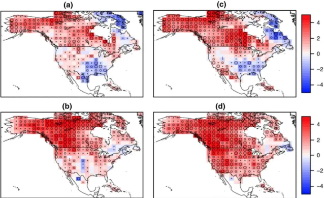
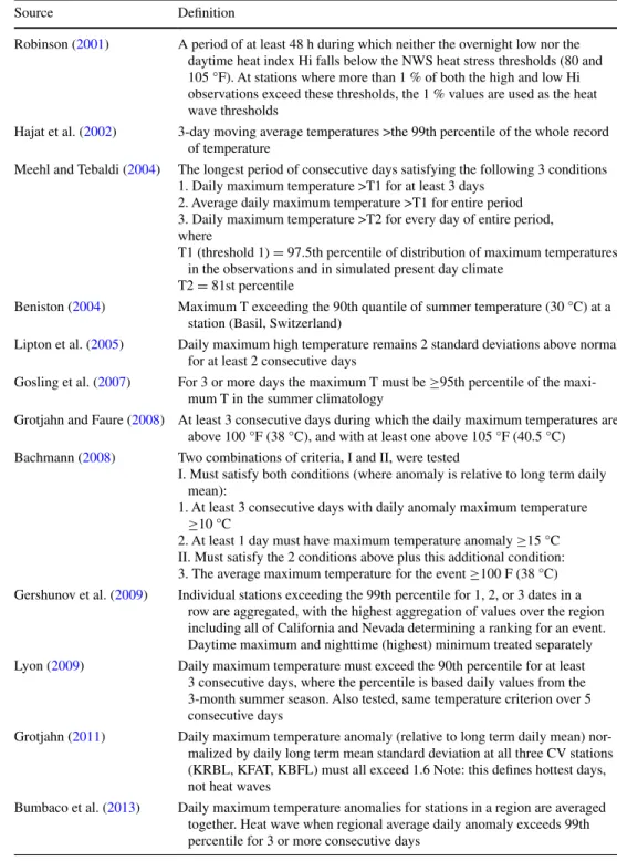
Figure 1 shows observed trends over North America from 1950 to 2007 in 20-year return values of the hottest/ coldest days and hottest/coldest nights. The temperature of very cold nights (Fig. 1d) exhibits pronounced warming over the entire continent as does the temperature of very cold days (Fig. 1b). The pattern of changes in the tempera-ture of very hot days (Fig. 1a) and very hot nights (Fig. 1c) follows that of average temperature change with strong cooling in the southeastern United States. This “warming hole” has been linked to sea surface temperature patterns in the equatorial Pacific (Meehl et al. 2007) and changes in anthropogenic aerosols in the eastern US (Leibensperger et al. 2012). Changes are more pronounced at the higher latitudes, except in Quebec and Newfoundland. This anal-ysis extends the work of Peterson et al. (2013) and uses annual anomalies to define the extreme indices. Although illustrative of the statistical techniques, analyses of annual-ized measures of extreme temperature cannot identify asso-ciated LSMPs that develop and dissipate on a much shorter time scale. Furthermore, events of high and low impact are better separated in seasonal analyses.

Table 1 Some temperature

related ETCCDI indices (Sillmann et al. 2013a)

For a complete list and formal definitions, see http://etccdi.pacificclimate.org/list_27_indices.shtml

ETCCDI index name Semi-formal definition Plain English

TX90p The percentage of days when the high temperature is greater than 90 % of those in reference period

Hot days

TX10p The percentage of days when the high temperature is less than 10 % of those in reference period

Cold days TN90p The percentage of days when the low temperature is greater

than 90 % of those in reference period

Hot nights TN10p The percentage of days when the low temperature is less

than 10 % of those in reference period

Cold nights TXx Monthly or seasonal maximum of daily maximum

temperature

Hottest day TXn Monthly or seasonal minimum of daily maximum

temperature

Coldest day TNx Monthly or seasonal maximum of daily minimum

temperature

Hottest night TNn Monthly or seasonal minimum of daily minimum

temperature

Coldest night

HWDI Heat Wave Duration Index Length of a heat wave

CWDI Cold Wave Duration Index Length of a cold spell

2.2 Application of extreme value statistical techniques

The observed changes in Fig. 1 are calculated using a time-dependent point process approach to fit “peaks over threshold” statistical models (Coles 2001). In this case, the extension of stationary extreme value methods to a time-dependent formalism used time as a “covariate” quantity to the ETCCDI indices (Kharin et al. 2013). A princi-pal advantage of a fully time dependent formalism over a quasi-stationary approximation (Wehner 2004) is that the amount of data used to calculate extreme value parameters is substantially increased, resulting in higher quality fitted distributions and hence more accurate estimates of long period return values. Calculations involving climate model output gain additional statistical accuracy by using multiple realizations from ensembles of simulations, provided they are independent and identically distributed.

The “block maxima” and “peaks over threshold” meth-ods to fit the tails of the distributions of random variables are asymptotic formalisms (Coles 2001). In this terminol-ogy, “block maxima” refers to use of only the maximum value during each “block” of time, usually a single season or year. The resulting generalized extreme value (GEV) or

Poisson and generalized Pareto distributions (GPDs) are both three parameter functions and can be transformed between each other. Hence provided that the data used to fit a distribution are in the “asymptotic regime”, i.e. far out in the tail of the distribution, the two methods are equiva-lent. Uncertainty in the estimate of long period tempera-ture return values resulting from limited sample size can be appreciable and may be as large as that from unforced inter-nal variability (Wehner 2010). However, variations in these estimates from multi-model datasets such as CMIP3/5 are generally significantly larger.

Confidence in the estimates of the statistical proper-ties of the tail of the parent distribution of a random vari-able can be ascertained by exploring the sensitivity to the sample size used to fit the extreme value distribution. For block maxima methods, the length of the block is a sea-son (or effectively so for temperature if the block length is a year). Lengthening the block makes the sample size smaller; shortening it makes the sample size larger since only one extreme value is drawn from each block. Such sensitivities are somewhat more straightforward to explore with peaks over threshold (POT) methods. Typical thresh-olds may be chosen between 80 and 99 % depending on

Fig. 1 Change over 1950–2007 in estimated 20-year annual return

values (°C) for a hot tail of daily maximum temperature (TXx), b cold tail of daily maximum temperature (TXn) c hot tail of daily minimum temperature (TNx) and d cold tail of daily minimum tem-perature (TNn). Results are based on fitting extreme value statistical models with a linear trend in the location parameter to exceedances of a location-specific threshold (greater than the 99th percentile for upper tail and less than the 1th percentile for lower tail). As this

analysis was based on anomalies with respect to average values for that time of year, hot minimum temperature values, for example, are just as likely to occur in winter as in summer. The circles indicate the z-score for the estimated change (estimate divided by its standard error), with absolute z-scores exceeding 1, 2, and 3 indicated by open circles of increasing size. Higher z-score indicates greater statistical significance

the size of the parent distribution that the extreme values are drawn from. However, standard POT methods may not discriminate between extreme values that occur at succes-sive dates when the individual extreme values may not be truly independent. In these cases, declustering techniques (Coles 2001) are applied to avoid biased (low) estimates of the uncertainty. The trends in extreme temperature shown in Fig. 1 are calculated using such a declustering technique and a POT formalism with time as a linear covariate. An alternative approach retains possibly dependent consecutive extremes, adjusting the estimates of uncertainty through either resampling or more advanced techniques for quan-tifying extremal dependence (e.g., Fawcett and Walshaw

2012). Furthermore, LSMPs responsible for extreme events can be formed using only the dates of the onset of the event (e.g. Grotjahn and Faure 2008; Bumbaco et al. 2013) reducing the risk of autocorrelated extremes. In the cited studies, a 5 day gap was typically required between events. Low frequency factors (or climate modes), such as ENSO, are best treated using the previously mentioned covariate techniques.

Some of the advantages and challenges of applying sta-tistical methods based on extreme value theory to analyze non-stationary climate extremes have been pointed out previously (e.g., Katz 2010), but are still not necessarily well appreciated by the climate science community. Con-ventional approaches tend to be either: (1) less informa-tive (e.g., analyzing only the frequency of exceeding a high threshold, not the excess over the threshold and not meas-uring the intensity of the event); or (2) less realistic (e.g., based on assumed distributions such as the normal that may fit the overall data well, but not necessarily the tails). When relating extremes to LSMPs, standard regression approaches would not quantify the uncertainty in the rela-tionship as realistically as using extremal distributions with covariates. Challenges in extreme value methods include specifying the dependence on LSMPs of the parameters of the extremal distributions in a manner consistent with our dynamical understanding. Moreover, heat waves and CAOs are relatively complex forms of extreme events, some of whose characteristics can be challenging to incorporate into the framework of extreme value statistics (Furrer et al.

2010). Finally, another advantage of the POT approach over the block maxima approach is being able to incorpo-rate daily indices of LSMPs as covariates (not just monthly or seasonally aggregated indices).

2.3 Identification of LSMPs related to extreme temperatures

Several methods have been used to identify LSMPs that occur in association with extreme temperature events. These methods and their properties are summarized in

Table 2. The text summarizes each method, its advantages and its disadvantages.

2.3.1 Composites

Composite methods define the LSMP using a target ensem-ble average. The values at a grid point for a field on speci-fied ‘target’ dates are averaged together. These dates might be when a temperature event begins (onset dates) defined as when some parameter(s) first meet some threshold and duration criteria. Table 3 illustrates various threshold and duration criteria that have been used to identify short-term extremely hot events. The different definitions yield some-what different dates and results. A definition using a physi-ological hazard (Robinson 2001) might not be satisfied at night in the coastal and some inland regions of the West, even though the daytime temperature threshold is well exceeded. Lower thresholds (90th percentile) generate more events thus increasing the sample size that can improve the statistical fit, though the behavior of the highest 1 % may not be well fit. Similarly, the number of stations (or the size of the area over which those stations occur) impacts which dates are identified, even for regions that would seem to be meteorologically consistent; for example, which sta-tions and how many are included from the Central Valley of California changes which dates exceed a threshold. Also, different definitions target different purposes: Grotjahn and Faure were interested in the LSMPs at the onset of the hot-test events while Meehl and Tebaldi were interested in find-ing the longest duration events of some importance. The number of dates averaged equals the number of ensemble members.

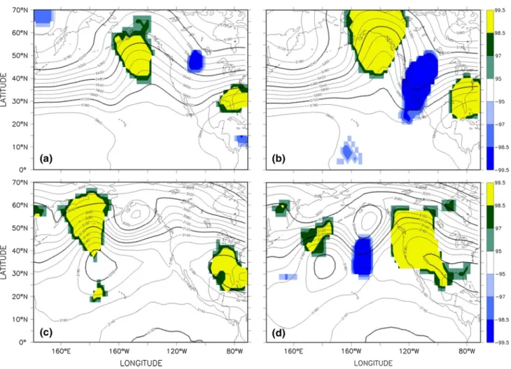
Compositing has several advantages. One can track LSMP formation by compositing fields with respect to the onset time of each event. Meteorologically relevant full fields (or anomalies) are obtained and composite analyses are constructed to obtain information on the synoptic and dynamical time evolution. The method is non-parametric in that it does not make any assumption about the pattern or the event statistics. Unlike some other methods, criteria can be applied (typically a minimum waiting period between events) to ensure events are independent. Significance can be assessed using a bootstrap resampling procedure where the target ensemble value at a grid point is compared to the distribution of values at that grid point found from a large number of ‘random ensembles’ (each of which uses the same number but randomly-chosen dates). Values above (or below) a threshold of the random ensemble distribution imply significantly high (low) values at that grid point. For example, a target ensemble value equal or higher than the top 10 of 1000 random ensemble values at that point is sig-nificant at approximately the 99 % level. Figure 2 shows the LSMPs for California Central Valley cold air outbreaks

Table

2

A summary of v

arious methodologies used to identify lar

ge scale meteorological patterns (LSMPs)

Method (e xample reference) Approach Attrib utes Cautions Significance testing

Composites (e.g. Grotjahn and F

aure

2008

)

A

verage together an ‘ensemble’ of maps on pre-identified dates As with some other procedures described here, it is important to assess ho

w independent the dates

are, e.g. consulting the autocor

-relation Ensemble a verage pro vides ph ysical

insights. Can be used to e

xamine

patterns leading up to and subse

-quent to the e

vent onset by shifting

dates used. Non-parametric in making no assumption about the pattern.

The dates can be chosen to

be independent

Must identify the e

vent dates

beforehand. Only finds one a

ver

-age unless indi

vidual members of

ensemble e

xamined and grouped

when choosing which dates are in which a

verage

Bootstrap resampling can compare ensemble a

verage to man

y random

ensemble a

verages (e.g. Grotjahn

and F

aure

2008

). Need lar

ger

sample size or another method to assess consistenc

y (e.g. sign counts:

Grotjahn

2011

)

Re

gression _{(e.g. Lau and Nath}

2012

)

Fit a re

gression line (polynomial in

the predictand) to a time series of a predictor at each grid point

Pattern pro

vides ph

ysical insights

Parametric in assuming a specific re

gression line (polynomial).

Can be used to e

xamine patterns

leading up to dates chosen e

vent if

ev

ent lasts for one time sample

Fit of re

gression line (polynomial)

to e

xtreme v

alues may be notably

altered by the choice of the poly

-nomial assumed. Only finds one pattern. Does not incorporate time threshold criteria (e.g. e

vent must

last >2

days)

T

reats all dates as

independent, which the

y might not

be. Does not separate onset from other days during an e

vent (e.g.

mixing onset with dates during the event). Ho

we

ver

, lo

w pass filtering

sometimes used to aggre

gate the

mixture of onset and during-e

vent

dates

Significance can be estimated by rejecting a null h

ypothesis about

the coefficients. based on where the regression line v

alues are higher (or

lo

wer) than a specified threshold of

the predictand v alues EOFs or PCs (W u et al. 2012 )

Calculate the eigen

vectors of a space-weighted co variance (between v alues at dif ferent grid

points) matrix. If only inputting extreme dates, then it is impor

-tant to assess ho

w independent

the dates are, e.g. consulting the autocorrelation Finds multiple patterns, each of which is orthogonal (not a subset) of another pattern. Can identify fraction of v

ariability that is due to

that EOF/PC. Most often used with filtered data to find leading lo

w

frequenc

y structures

Not suitable when applied to all data as the leading EOFs will be common patterns not necessar

-ily rele

vant to rare e

vents. EOFs

more useful when calculated only from data on e

vent dates identified

beforehand. Eigen

vectors may

not be sufficiently distinct.

The

patterns found may depend on domain chosen, though EOF ‘rota

-tion’

may help. Each EOF e

xplains

only a fraction of the v

ariance

and so no single EOF might be an LSMP thereby limiting ph

ysical

insight

No inherent significance test since the EOFs (or PCs) may not represent an actual weather pattern.

The

amount of v

ariance associated with

Table 2 continued Method (e xample reference) Approach Attrib utes Cautions Significance testing SOMs (e.g. He witson and Crane 2002 )

Obtain the distrib

ution of patterns

co

vered by a set of input maps,

using neural-net training

Resultant maps span the pattern space of input fields, represent nodes of a continuous pattern distrib

ution, and can be related to

a transformation of rotated EOFs back to ph

ysical space

Results can be sensiti

ve to the

domain used for pattern analysis. Care needed to ensure appropriate resolution of LSMP space. Lo

w

resolution can f

ail to resolv

e pat

-tern features important for e

xtreme

ev

ents/Ov

erly fine resolution

undermines significance testing

Bootstrapping methods can compare frequenc

y distrib

utions of e

xtreme-ev

ent days in LSMP space with ran

-dom sampling of all days to indicate significance of e

vent clustering in

subre

gions of the full pattern space.

(e.g. Cassano et

al.

2007

)

Clustering analysis (e.g. Stephanon et

al.

2012

)

Assigning e

vents to K clusters so

that it minimizes total sum of the generalized Euclidian distance between patterns in a cluster (Spath

1985

; Seber

2008

). If only

inputting e

xtreme dates, then it is

important to assess ho

w independ

-ent the dates are, e.g. consulting the autocorrelation

Objecti

vely classify e

vents and find

relating LSMPs that pro

vide ph

ysi

-cal insight

No assumptions about the patterns such as orthogonality and sym

-metry The number K of LSMP clusters can be some

what arbitrary since K is

pre-specified, b

ut the ‘dissimilarity

inde

x’

can estimate the separation

between clusters for dif

ferent K

and help optimize the v

alue of K.

Lar

ger separation between clusters

is preferred and generally declines as K increases. Optimal K can be unclear for some situations. Significance of classification stability can be obtained from Monte Carlo test by rejecting the null h

ypothesis

that the v

erification period tempera

-ture e

xtreme cannot be classified in

the clusters obtained from remain

-ing periods. Lee and Grotjahn (2015

) use bootstrap method

(random ensembles same number of members as the cluster) to identify what parts of each cluster a

verage

are notable for the e

xtreme e

vent

Machine learning (Salakhutdino

v

and Hinton

2012

)

T

rain a multi-layer neural netw

ork

on a dataset.

T

raining is done one

layer at a time, with spatio-tempo

-ral patches at the bottom layer

, and

class labels being assigned at the top layer

Deep Belief Netw

orks ha

ve pro

ved

to be po

werful in capturing a range

of patterns. It is lik

ely that the

y will e xtract in variant patterns as well as anomalies These techniques ha ve produced

state-of-the-art results in computer vision and speech recognition tasks.

The

y ha

ve not yet been

applied to climate datasets

Has not been conducted in the conte

xt

of climate/LSMP applications. Clas

-sification performance of method has been conducted e

xtensi

vely for

and heat waves obtained by this method, including boot-strap resampling significance.

Compositing has some disadvantages that can be addressed. The identification of the extreme event dates must be done separately and before the compositing. The composite produces one target ensemble average (for a specific field and level) for each set of target dates. If more than one LSMP can produce the extreme event, then that must be identified either with one or more additional criteria when choosing dates or identified by

examining (perhaps qualitatively) the maps for each indi-vidual member of the target ensemble. A procedure like adding the number of positive and subtracting the num-ber of negative anomaly values at a grid point in the tar-get ensemble members (called the ‘sign count’ in Grot-jahn 2011) can assist with identifying multiple patterns. (If the sign count equals the number of ensemble mem-bers, then all members have the same sign of the anomaly field at that location.) Lee and Grotjahn (2015) apply a cluster analysis to distinctly different parts of LSMPs

Table 3 Sampling of Various

Criteria Used in Heat Wave and Hottest Day Definitions

Source Definition

Robinson (2001) A period of at least 48 h during which neither the overnight low nor the daytime heat index Hi falls below the NWS heat stress thresholds (80 and 105 °F). At stations where more than 1 % of both the high and low Hi observations exceed these thresholds, the 1 % values are used as the heat wave thresholds

Hajat et al. (2002) 3-day moving average temperatures >the 99th percentile of the whole record of temperature

Meehl and Tebaldi (2004) The longest period of consecutive days satisfying the following 3 conditions 1. Daily maximum temperature >T1 for at least 3 days

2. Average daily maximum temperature >T1 for entire period 3. Daily maximum temperature >T2 for every day of entire period, where

T1 (threshold 1) = 97.5th percentile of distribution of maximum temperatures in the observations and in simulated present day climate

T2 = 81st percentile

Beniston (2004) Maximum T exceeding the 90th quantile of summer temperature (30 °C) at a station (Basil, Switzerland)

Lipton et al. (2005) Daily maximum high temperature remains 2 standard deviations above normal for at least 2 consecutive days

Gosling et al. (2007) For 3 or more days the maximum T must be ≥95th percentile of the maxi-mum T in the summer climatology

Grotjahn and Faure (2008) At least 3 consecutive days during which the daily maximum temperatures are above 100 °F (38 °C), and with at least one above 105 °F (40.5 °C)

Bachmann (2008) Two combinations of criteria, I and II, were tested

I. Must satisfy both conditions (where anomaly is relative to long term daily mean):

1. At least 3 consecutive days with daily anomaly maximum temperature ≥10 °C

2. At least 1 day must have maximum temperature anomaly _≥15 °C II. Must satisfy the 2 conditions above plus this additional condition: 3. The average maximum temperature for the event _≥100 F (38 °C) Gershunov et al. (2009) Individual stations exceeding the 99th percentile for 1, 2, or 3 dates in a

row are aggregated, with the highest aggregation of values over the region including all of California and Nevada determining a ranking for an event. Daytime maximum and nighttime (highest) minimum treated separately Lyon (2009) Daily maximum temperature must exceed the 90th percentile for at least

3 consecutive days, where the percentile is based daily values from the 3-month summer season. Also tested, same temperature criterion over 5 consecutive days

Grotjahn (2011) Daily maximum temperature anomaly (relative to long term daily mean) nor-malized by daily long term mean standard deviation at all three CV stations (KRBL, KFAT, KBFL) must all exceed 1.6 Note: this defines hottest days, not heat waves

Bumbaco et al. (2013) Daily maximum temperature anomalies for stations in a region are averaged together. Heat wave when regional average daily anomaly exceeds 99th percentile for 3 or more consecutive days

prior to California heat waves and identify two ways the onset LSMPs form.

2.3.2 Regression

Regression estimates one quantity (the predictand) using a function of one or more other quantities (the predictors). The method is often parametric in assuming a specific func-tion relates a predictor to the predictand (but nonparametric methods exist, too). An example predictor might be daily minimum surface temperature and the predictand might be 700 hPa level meridional wind. At each grid point the value of the predictand can be estimated using a polyno-mial function of the predictor, where the coefficients of that polynomial are calculated to minimize a squared difference between actual predictand values and polynomial values at that grid point. In general, the coefficients differ from grid point to grid point. To find the LSMP in this example of

extreme cold events, the polynomial can be used to con-struct the predictand at each grid point using a predictor value such as two standard deviations below normal.

The pattern obtained by regression can provide physical insights by directly linking the patterns in the predictand to extremes in the predictor. For example, lower tropospheric (700 hPa) winds prior to a California CAO flow from northern Alaska and northern western Canada to reach Cal-ifornia without crossing over the Pacific Ocean. Regression can be used to examine patterns leading up to (or after) event onset dates by offsetting in time the predictor values from the predictand values when calculating the regression coefficients. The LSMP is again the resultant predictand when the predictor is at some specified value (e.g. predictor equals two standard deviations below normal). Significance can be estimated by rejecting a null hypothesis (e.g. that the regression coefficient is zero at the 1 % level using a student’s t test).

Fig. 2 Example large scale meteorological patterns (LSMPs)

obtained as target ensemble mean composites for two types of Cali-fornia Central valley extreme events. Cold air outbreaks in winter (DJF) at a 72 h prior and b at onset of the events are shown in the 500 hPa geopotential height field. Heat waves during summer (JJAS),

c 36 h prior and d at the onset are shown in the 700 hPa geopotential height field. Shading indicates significance at the highest or lowest 5 % level, with the innermost shading significant at the 1.5 % level. Further discussion is in Grotjahn and Faure (2008)

One disadvantage of regression is that the assumption of a specific polynomial to represent how the predictand var-ies relative to the predictor. The fit of the regression line (polynomial) to extreme values may be notably altered by the order of the polynomial assumed. Regression, like com-posites, only finds one pattern. Regression does not incor-porate event duration criteria (such as: the event must last at least 3 days). Regression treats all dates as independent, which they are not likely to be; however this can be some-what mitigated by sub-sampling the data (e.g. only use every fifth day). Subsampling might be combined with low pass filtering to aggregate the mixture of onset and during-event dates. Another disadvantage is that a portion of the pattern may be highly significant but only have small cor-relation to the predictor.

2.3.3 Empirical orthogonal functions

Empirical orthogonal functions (EOFs) or principal com-ponents (PCs) can be used to identify LSMPs for extreme events. EOFs are the eigenfunctions of a matrix formed from the covariance between grid points on maps. EOFs from all maps in a time record will be ordered based on the eigenfunctions responsible for the largest amount of variance between time samples. Such eigenfunctions are the most common modes of variability and so not likely to be LSMPs of extreme events that are rare (except as men-tioned in the introduction). However, EOFs can be formed only from maps selected in reference to an extreme event, such as maps only on the target dates of events onset. (EOFs of common low frequency modes may influence short-term extreme events focused on in this paper, as dis-cussed in Sect. 3.1.) Weighting can be used for a variable grid spacing (such as occurs when using equal intervals of longitude across a range of latitudes).

An advantage of EOFs/PCs is the method finds multi-ple patterns, each of which is orthogonal (not a subset) of another pattern. The method can calculate the fraction of variability that is due to each EOF/PC. This approach is most often used with filtered data to find low frequency structures. This method is suitable for finding patterns lead-ing up to and after the event by shiftlead-ing the dates chosen by the event criteria (and only using those dates). In a study of California Central Valley hot spells, Grotjahn (2011) found the leading EOF based on dates satisfying the criteria in Table 3 to be very similar to the corresponding ensemble mean composite.

A disadvantage is that the patterns found may depend on the domain chosen, though EOF ‘rotation’ may help. Also, each EOF may explain only a small fraction of the variance and no single EOF might be an LSMP thereby limiting physical insight. Different leading EOFs/PCs might have structures influenced by the required orthogonality and

possibly not a pattern that occurs during an event. While the amount of variance associated with a given EOF is used to indicate the importance of the EOF, there is no inherent statistical significance test. Hence it can be unclear what portions of the EOF are significantly associated with the extreme event and what parts are not (and happen to reflect limited variation in the finite sample).

2.3.4 Clustering analysis

Clustering analysis is terminology indicating a widely used partitioning procedure that identifies separate groups of objects having common structural elements. Clustering analysis has been used to classify distinct sets of LSMPs associated with extreme events (Park et al. 2011; Stepha-non et al. 2012). When we have 100 historical hot spell events over a given region, not all extreme events may have the same LSMP on or prior to their onset. Some events may have a wave-like height field, others may have a dipole pat-tern, and still others may have a third pattern. Although detailed grouping procedures vary for every clustering technique, the basic concept is to minimize the overall dis-tance between patterns among events in resultant groups. For example, the k-means clustering technique applies an iterative algorithm in which events are moved from one group to another until there is no additional improvement in minimizing the squared Euclidean point-to-centroid dis-tance in a group (Spath 1985; Seber 2008), where each cen-troid is the mean of the patterns in its cluster.

Output of clustering analysis is just the average field of events in each cluster, similar to the output from composite analysis. Unlike composite analysis in which members of clusters are pre-identified, the essential point of clustering analysis is to objectively classify events based on spatial pattern similarity. By applying cluster analysis to group similar onset patterns, one can isolate distinct dynamical origins of different extreme temperature events. Another advantage is that resultant clusters are based on physical maps without assumptions of orthogonality and symmetry such as in the mode separation by EOF/REOF. The robust-ness of a hot spell classification can be tested by a Monte Carlo test as follows. First one calculates a stability score that is the ratio of the number of verification period heat waves that are correctly attributed over the total number heat waves in the cluster. Second one estimates the prob-ability density function (PDeF) of the null hypothesis that cluster assignment is purely random. Significance of each cluster can be estimated by rejecting a null hypothesis (e.g. stability score is located within highest 99 % of PDeF).

A disadvantage of clustering analysis is that one pre-specifies the number of clusters (e.g. k in k-means cluster-ing). Determining the number k is subjective if one does not have sufficient prior knowledge of related physical

patterns. There are several statistics to check the optimal number of k such as ‘distance of dissimilarity’ (Stephanon et al. 2012). Another disadvantage is the ambiguity of clus-ter assignment for certain events. Another disadvantage is the patterns of such events cannot be assigned clearly to one group over another group. Part of a pattern may resem-ble Cluster #1, while another part may be more similar to Cluster #2. To avoid ascribing some marginal events to spe-cific clusters, probabilistic clustering methods (e.g. Smyth et al. 1999) are developed, which suggests the possibility (e.g. percentage) that an event could be assigned to each cluster rather than assigning it only to one cluster. If one increases the cluster number, one can expect to decrease such ambiguity in classification. However, the point of clustering analysis is to give a physical insight with mini-mal groups and not to interpret every single episode.

2.3.5 Self‑organizing maps

Self-organizing maps (SOMs; Kohonen 1995) are two-dimensional arrays of maps that display characteristic behavior patterns of a field (e.g., Cavazos 2000; Hewit-son and Crane 2006; Gutowski et al. 2004; Cassano et al.

2007). The SOM array is a discretization of the continuous

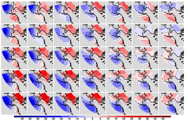
pattern space occupied by the field examined. Thus, in con-trast to clustering analysis, SOMs do not assume a clump-ing together of patterns, though such behavior can emerge if present in the input data. Figure 3 gives an example of a SOM array of synoptic weather patterns in sea level pres-sure over a region centered on Alaska. Individual maps in the array represent nodes in a projection of this continuous space onto a two-dimensional surface, with the size of the array determined by the degree of spatial discretization of the SOM space one “feels” is needed for the analysis at hand. The two dimensions show the two primary pattern transitions for the field examined. Although one could, in principle, use more than two dimensions, typical practice in climatological work has used only two.

The input maps themselves determine the degree and types of pattern transitions, hence the “self-organizing” nature of the resulting array. The SOM node array is trained on a sequence of input maps through an artificial neural net technique. The SOM array does not necessar-ily favor the largest scales in the input data, but rather the scales most relevant to the field for the domain and reso-lution examined. Consequently, SOMs can extract nonlin-ear pattern changes in fields, such as shifts in strong gra-dients. In addition, the pattern at each node is essentially

Fig. 3 Self-organizing map of synoptic weather patterns in a region

focused on Alaska. The SOM array maps give the departure (in hPa) of sea level pressure (SLP) from the domain averaged sea level pres-sure. The SOM used daily December–January–February (DJF) SLP

for 1997–2007 from ERA-interim reanalyses and output from a regional climate model. Locations with elevation exceeding 500 m are not included in the maps to avoid using SLP in regions strongly influenced by methods used to extrapolate SLP from surface pressure

a composite of input maps with similar spatial distribution for the field examined, so that patterns in the SOM array show archetypal patterns of the field examined and directly lend themselves to physical interpretation. Typically, the SOM array displays features having the highest temporal variance in the input data. From this perspective, the SOM array is roughly akin to a transformation of a rotated EOF from spectral space back to physical space.

An advantage of SOMs is that one can identify the nodes where extreme events occur frequently and thus the physical behavior yielding extremes. For example, extreme events may tend to cluster in a small portion of SOM space, thereby allowing identification of LSMPs yielding extreme events. A further advantage is that if more than one group emerges in the SOM-space frequency distribution, then the grouping provides a SOM-determined segregation of dif-ferent types of extreme events. One can then focus analy-sis and composites of additional fields (e.g., precipitation, winds, temperature) on only events of the same type. For example, Cassano et al. (2006) used SOMs of sea-level pressure patterns over Alaska to determine which synoptic weather patterns were responsible for extreme wind and temperature events at Barrow, Alaska. They then found robust links between these large-scale synoptic weather patterns and local weather features (precipitation, winds, and temperature). One can construct estimates of the sig-nificance of differences in frequency distributions in SOM space through bootstrapping procedures to estimate the likelihood that frequency distributions are not simply the result of random, finite sampling of the pattern space. Thus one can compare frequency distributions between a present and projected climate to assess potential climate changes in LSMPs, or between observational and model climates to assess similarity of observed and simulated LSMPs yield-ing extremes.

A disadvantage of SOMs is that the array size is pre-determined by the user, and there is no clear, objective guideline for selecting array size. There are, however, some factors that can affect the array-size choice. The issue of significance limits the degree of discretization (number of nodes) one applies to the SOM space. Fine discretization will allow apparent detection of small differences in how different data sets occupy pattern space, but fine discre-tization will also render very noisy frequency distribution functions of the fields in SOM space, thus undermining detection of any significant differences. Coarse discretiza-tion limits the ability of the SOM procedure to resolve fea-tures producing the extreme events, so a further disadvan-tage is that an insufficient array size may obscure grouping that may be present in the data. The training method also requires specification of parameters that govern the training process. A well-trained SOM is insensitive to these choices, but care is needed to ensure such a result. In addition, like

some of the other methods described here, the extreme events are defined separately from the SOM analysis.

2.3.6 Machine learning and other advanced techniques

Looking to the future, we note that substantial progress has been made in the field of machine learning for extract-ing patterns from Big Data. Commercial organizations such as Google and Facebook rely on sophisticated, scal-able analytics techniques for mining web-scale datasets. Both supervised and unsupervised machine learning tools could play an important role in extracting spatio-temporal patterns from climate datasets. The technique Deep Belief Networks (Salakhutdinov and Hinton 2012) has been applied with tremendous success to classifying objects in digital images (Krizhevsky et al. 2012) and speech recogni-tion (Hinton et al. 2012). These methods have substantially outperformed existing techniques in the field with the same underlying learning algorithm. While these techniques have not yet been adapted for a multivariate spatio-temporal dataset (such as in climate), research efforts are currently underway to evaluate the performance of such methods in extracting patterns as well as anomalies from datasets. It is too early to discern pros and cons fully for such methods.

2.4 Including large scale patterns in extreme statistics

Application of covariates in extreme value methods (termed “conditional extreme value analysis”) is relatively new to the climate science community, although it has been avail-able to the larger statistics community for some time (Coles

2001). The basic idea of conditional extreme value analy-sis is to allow the extremal distribution to be dynamic; that is, shifting depending on the observed value of an index of a climate mode or LSMP (the index would be an example of a “covariate”). The book by Coles includes an example in which annual maximum sea level is related to a climate mode, the Southern Oscillation. In their study of changes in extreme daily temperatures, Brown et al. (2008) used the NAO as a covariate in addition to a trend component.

Such techniques have proven useful in connecting extreme temperatures to LSMPs. Sillmann and Croci-Maspoli (2009) and Sillmann et al. (2011) used a blocking index as a covariate for extremely cold European winter temperatures and found that extreme value distributions (based on block minima) were better fit and long period return values were somewhat colder. Furthermore, they concluded that projected future extremely cold events in Europe were less influenced by atmospheric block-ing because of projected shifts in North Atlantic blockblock-ing patterns. Photiadou et al. (2014) used a similar technique (but based on the POT approach rather than block max-ima) to connect blocking and other indices to European

high temperature events finding that while El Nino/South-ern Oscillation (ENSO) does not exert much influence on extremely high temperature magnitudes or duration, the North Atlantic Oscillation (NAO) and atmospheric block-ing do. However to date, such covariate techniques relat-ing atmospheric blockrelat-ing to extreme temperatures have not been applied to North America. Many physically based covariate quantities potentially offer insight into the mecha-nisms behind extreme temperature events and the response to changes in the average climate. Good North American candidates for covariates include indices measuring modes of natural variability such as those describing the ENSO, the Pacific Decadal Oscillation (PDO), the NAO, the North Atlantic Subtropical High (NASH), and various blocking indices.

The ETCCDI indices were designed for climate change detection and attribution purposes rather than for explor-ing the mechanisms causexplor-ing extreme events. They are not ideal for connecting extreme temperature events to LSMPs and they are not descriptive of particularly rare events. However, ETCCDI indices are designed to be robust over the observational record and have been calculated and described for CMIP5 models by Sillmann et al. (2013a) (see Table 1). ETCCDI indices are intended to be applied globally and be meaningful in areas of sparse observations. The relatively dense network of North American observa-tions since the beginning of the twentieth century permits the construction of more specialized LSMP extreme indices linked to specific extreme events. Grotjahn (2011) defines an index that is an unnormalized projection of key parts of a target ensemble LSMP onto a daily map of the cor-responding variable. (He combined such projections onto 850 hPa temperature and 700 hPa meridional wind to form his ‘circulation index’.) His target ensemble members are from dates satisfying criteria listed in Table 3. The key parts of the fields used are those where all the extreme events in the training period were consistent, at least in having the same anomaly sign. Grotjahn (2011) found that extreme values of such an index (based on upper air data) occurred on many of the same dates as extreme values of surface sta-tions in the California Central Valley (CCV). Statistically significant relationships exist between extreme values of this circulation index and both the rate of CCV daily maxi-mum temperature exceeding a high threshold and the distri-bution of the excess over the threshold (Katz and Grotjahn

2014). Grotjahn (2013) used such an index to show that a particular climate model was notably under-predicting the occurrence frequency (by half) of CCV hot spells. Grotjahn (2015) used such an index to show how that same model compared with a 55 year historical record and what the model implied for CCV hot spells during the last half of the twentyfirst century under two representative concentration pathways (RCPs) of greenhouse gases.

3 Large scale meteorological patterns related to extreme temperature events

Intraseasonal extreme temperature events (ETEs) are almost always associated with regional air mass excursions induced by circulation anomalies that are part of large-scale meteorological patterns (LSMPs). LSMPs can include syn-optic features (e.g., midlatitude cyclones; Konrad 1996) that enhance the ETE and often with scales similar to a tel-econnection pattern (though the nodes may not align and ETE onset, itself, may impact the teleconnection pattern, Cellitti et al. 2006). In some cases, the LSMP is interpreted as a juxtaposition of teleconnection patterns that leads to ETE events (Lim and Kim 2013). Heuristically, the role of LSMPs in producing ETEs could be considered the result of either (1) a direct contribution to the large-scale circula-tion that facilitates the air mass excursion or (2) the indi-rect modulation of sub-scale variability, such as regional modulation of storm track behavior by blocking patterns. Besides such dynamically driven impacts, there exist pos-sible local impacts related to the interaction of the LSMP with local topography or coastline features, leading to pos-sible local symmetries in the response pattern (e.g., Loikith and Broccoli 2012). Current knowledge of the remote forc-ing, dynamics and local forcing of LSMPs associated with ETEs is summarized next.

3.1 Remote forcing of LSMPs and ETEs

3.1.1 Connection to low frequency modes of climate variability

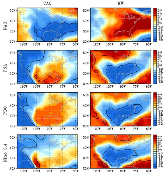
Numerous observational studies have ascertained that ETE behavior is modulated by recurring large scale telecon-nection patterns, particularly during winter. On intrasea-sonal time scales there is a substantial modulation of North American ETEs during winter by the Pacific-North Ameri-can (PNA) pattern, North Atlantic (or Arctic) Oscillation (NAO or AO) and blocking patterns (Walsh et al. 2001; Cellitti et al. 2006; Guirguis et al. 2011). On interannual and longer time scales additional climate modes such as El Nino-Southern Oscillation (ENSO) and the Pacific Decadal Oscillation (PDO) are also implicated (Westby et al. 2013). General relationships that have emerged from these statisti-cal analyses are illustrated in Fig. 4: The positive (negative) phase of the NAO favors the occurrence of warm (cold) events over the eastern (southeastern) United States. The positive (negative) phase of the PNA tends to favor cold events over the southeastern (northwestern) US. These con-nections to climate modes are neither unique nor independ-ent. For example, the regional influence of the PNA pattern on ETEs largely mirrors that of both the PDO and ENSO (Fig. 4) since the midlatitude atmospheric signatures of

both ENSO and the PDO project on the PNA pattern. Also, the prevalence of atmospheric blocking patterns is intrin-sically linked to particular climate mode phases (Renwick and Wallace 1996).

There have been pronounced episodes of climate modes influencing ETEs during recent winters. Cold extremes over Europe and the southeastern United States during recent winters (2009–2010 and 2010–2011) were primar-ily accounted for by the anomalous blocking associated with persistent episodes of large amplitude negative phase of the NAO (Guirguis et al. 2011). There is also evidence of an important role for stationary Rossby wave patterns in contributing to North American temperature extremes during summer (Schubert et al. 2011; Wu et al. 2012). These wave patterns appear to arise from internal forcing

associated with intraseasonal transient eddies (Schubert et al. 2011).

As discussed above, two more commonly recognized remote influences upon North American ETEs are associ-ated with ENSO and the PDO (e.g., Westby et al. 2013), both involving local sea surface temperature anomalies and atmosphere–ocean coupling. These generally operate in conjunction with PNA-like teleconnection patterns that extend from the coupling region downstream into North America. Similar to the effect of climate modes, the impact of remote forcing upon warm season ETEs is partly lim-ited by the relative inactivity and spatial extent of climate modes, which serve as horizontal pathways for Rossby wave energy between the remote forcing region and the local surface response (Schubert et al. 2011).

Fig. 4 Correlation between the local seasonal impact of cold days

(left column) and warm days (right column) and the seasonal mean NAO (first row), PNA (second row), PDO (third row) and Niño 3.4

indices (fourth row) during winter, 1950–2011. The black contours encompass regions having correlations statistically significant at the 95 % confidence level (figure from Westby et al. 2013)

3.1.2 Connection to sea ice and snow cover

The atmospheric response to the Arctic sea ice reduction is thought to be Arctic warming and destabilization of the lower troposphere, increased cloudiness, and weakening of the poleward thickness gradient and polar jet stream (Fran-cis et al. 2009; Outten and Esau 2012). As the Arctic warms faster than lower latitudes (so-called Arctic Amplification), the meridional temperature gradient at higher latitudes is likely to weaken altering the polar jet stream according to thermal wind balance. Changes in the high latitude jet stream in turn have the potential to impact weather con-ditions at middle and high latitudes. For example, during winter an enhanced westerly jet over the North Atlantic can help maintain relatively mild conditions over northwest Europe via heat transport from the Atlantic. Cohen et al. (2014) review three “pathways” by which Arctic amplifica-tion may impact extreme weather events in mid-latitudes. In principle, Arctic amplification may lead to regional alterations in the structure of storm tracks, jet streams and planetary waves. In recent years, considerable attention has been focused on the role of Arctic amplification-induced changes to the jet stream (Francis and Vavrus 2012; Liu et al. 2012; Barnes 2013; Screen and Simmonds 2013). Francis and Vavrus (2012) found that a weaker zonal flow (i.e., polar jet) from weakened meridional temperature gradient slows the eastward Rossby wave progression and tends to create larger meridional excursions of height con-tours and associated temperature displacements resulting in a higher probability of extreme weather. In a similar vein, Liu et al. (2012) argue that the circulation change due to the decline of Arctic sea ice leads to more frequent events of atmospheric blocking that cause severe cold surges over large parts of northern continents. Francis et al. (2009), Overland and Wang (2010), Jaiser et al. (2012) and Lim et al. (2012) found that there is a delayed atmospheric response to the Arctic sea ice. Specifically, the Arctic sea ice extent in summer to fall influences the atmospheric cir-culation in the following winter over the northern mid- to high-latitudes, affecting the seasonal winter temperature and subseasonal warm/cold spells. Evidence presented in more recent studies (Barnes 2013; Screen and Simmonds

2013), however, suggests that the role of the mechanism put forth by Francis and Vavrus (2012) is uncertain at best. More generally, Cohen et al. (2014) conclude that our understanding of the mechanistic link between ongoing Arctic amplification and mid-latitude extreme weather is currently limited by shortcomings in relevant data records, physical models and dynamical understanding, itself. As such, the likely future impact of Arctic amplification upon extreme weather is highly uncertain.

Arctic amplification is also linked to long-term vari-ability in high latitude snow cover. An analogous linkage

between autumnal variability in Eurasian snow cover and wintertime ETE events over North America has been noted (Cohen and Jones 2011). In this case, autumnal snow cover anomalies induce a subsequent weakening of the strato-spheric polar vortex during winter which, in turn, leads to a persistent negative phase episode of the tropospheric AO favoring North American cold events (Cohen et al.

2007). In addition, there is evidence that the changing Arc-tic sea ice extent may be linked to changes in the autum-nal advance in Eurasian snow cover (Cohen et al. 2013). As for Arctic amplification, however, there is considerable uncertainty regarding the statistical robustness and physi-cal nature of the Eurasian snow cover influence upon mid-latitude extreme weather (Peings et al. 2013; Cohen et al.

2014).

3.1.3 Large‑scale climate “markers” for climate model assessment

Representation of fundamental climate modes One obvious essential minimum requirement for climate models to prop-erly represent the modulation of ETEs by climate modes is the extent to which the models are able to represent the primary climate modes, themselves. Thus, fundamental markers for model assessment are metrics that measure the representation of key extratropical climate modes including those internally forced on intraseasonal time scales (PNA, AO/NAO and atmospheric blocking) and those externally forced on longer time scales (the extratropical response to ENSO and the atmospheric part of the PDO). Atmospheric models have had historical difficulty in representing some types of intraseasonal low frequency variability (Black and Evans 1998). A particular problem is an under-representa-tion of atmospheric blocking activity (Scaife et al. 2010). In a similar vein, the representation of externally forced extratropical modes connected to ENSO and PDO depends on how well the coupled climate models simulate the asso-ciated oceanic phenomenological behavior.

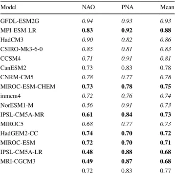
The Coupled Model Intercomparison Project (CMIP) provides an ideal resource for assessing the ability of mod-ern coupled climate models to represent the behavior of cli-mate modes. A recent analysis of CMIP5 models indicates that while most models studied perform well in represent-ing the basic aspects of the PNA pattern, a small subset of models have difficulty qualitatively replicating the NAO pattern (Lee and Black 2013; Table 4). Otherwise differ-ences among model patterns consist of horizontal shifts or amplitude variations in the circulation anomaly pattern fea-tures. CMIP5 models generally underestimate the regional frequency of winter blocking events while summertime blocking events occurring over the high latitude oceanic basins are typically overestimated (Masato et al. 2013). Conversely, Westby et al. (2013) found serious deficiencies