Modi
fi
ed kernel principal component analysis based on local structure
analysis and its application to nonlinear process fault diagnosis
Xiaogang Deng
a, Xuemin Tian
a, Sheng Chen
b,c,⁎
aCollege of Information and Control Engineering, China University of Petroleum (East China), Qingdao, Shandong 266555, China bElectronics and Computer Science, Faculty of Physical and Applied Sciences, University of Southampton, Southampton SO17 1BJ, UK c
Faculty of Engineering, King Abdulaziz University, Jeddah 21589, Saudi Arabia
a b s t r a c t
a r t i c l e i n f o
Article history:
Received 15 December 2011 Received in revised form 28 June 2013 Accepted 5 July 2013
Available online 16 July 2013 Keywords:
Kernel principal component analysis Local structure analysis
Fault diagnosis Fault detection
Fault identification
Nonlinear process
Traditional kernel principal component analysis (KPCA) concentrates on the global structure analysis of data sets but omits the local information which is also important for process monitoring and fault diagnosis. In this paper, a modified KPCA, referred to as the local KPCA (LKPCA), is proposed based on local structure analysis for nonlinear process fault diagnosis. In order to extract data feature better, local structure analysis is integrated within the KPCA, and this results in a new optimisation objective which naturally involves both global and local structure information. With the application of usual kernel trick, the optimisation problem is transformed into a generalised eigenvalue decomposition on the kernel matrix. For the purpose of fault detection, two mon-itoring statistics, known as theT2andQstatistics, are built based on the LKPCA model and con
fidence limit is computed by kernel density estimation. In order to identify fault variables, contribution plots for monitoring sta-tistics are constructed based on the idea of sensitivity analysis to locate the fault variables. Simulation using the Tennessee Eastman benchmark process shows that the proposed method outperforms the traditional KPCA, in terms of fault detection performance. The results obtained also demonstrate the potential of the proposed fault identification approach.
© 2013 Elsevier B.V. All rights reserved.
1. Introduction
The demands for improving product quality and ensuring process safety have stimulated the recent development of fault diagnosis techniques. As large amounts of data are available in modern pro-cess industry, data-driven methods based on the statistical propro-cess control theory have been one of the most fascinating topics in the process fault diagnosisfield. Principal component analysis (PCA) is a classical data-driven multivariate statistical method which has attracted much attention from researchers[1–3]. However, PCA is a linear projection method, which cannot effectively capture the nonlinear features existing in real industrial processes. In order to cope with this problem, many modified nonlinear PCA methods have been developed. Krammer[4]first studied a nonlinear PCA based on an auto-associative neural network. Dong and MacAvoy
[5]proposed the principal curve method as a nonlinear generalisa-tion of linear PCA. Hiden et al.[6]suggested a nonlinear PCA using genetic programming, while Geng and Zhu[7]presented an adap-tive nonlinear PCA based on an improved input training neural network.
More recently, the kernel PCA (KPCA) method has gained consid-erable interests in various researchfields. KPCA wasfirstly proposed in[8], which applies a kernel function to compute the nonlinear prin-cipal components. This method has been applied to process fault de-tection and diagnosis. Lee and co-authors[9,10]proposed the KPCA-basedT2andQstatistics for the fault detection of continuous and
batch processes. Cho et al.[11]and Choi et al.[12]formulated two fault identification strategies using KPCA. In order to analyse multi-scale data, multi-multi-scale KPCA methods were studied by combining the wavelet analysis and ensemble empirical mode decomposition
[13–16]. To improve the computation efficiency, Tian et al.[17]and Cui et al.[18]used feature sample selection to reduce the computa-tional complexity of calculating the kernel matrix in KPCA. Nguyen and Golinval [19]applied the KPCA to detect mechanical system faults by comparing the subspace angle between a reference and the current state. Considering the dynamic property of process data, Jia and co-authors[20]developed a dynamic KPCA method by integrating the kernel PCA and ARMAX time series model, while Zhang et al.[21]discussed a multi-block KPCA for large-scale cesses. For effective monitoring of nonlinear and nonstationary pro-cesses, the work[22]proposed a variable window adaptive KPCA based on a fast block adaptation. Cao et al.[23]formulated the mod-ularity of kernel methods for chemical data modelling, while Fu et al.
[24]applied KPCA to capture the latent structure of training data for building a two-step nonlinear classification algorithm. It can be seen
⁎ Corresponding author at: Electronics and Computer Science, Faculty of Physical and
Applied Sciences, University of Southampton, Southampton SO17 1BJ, UK. E-mail address:[email protected](S. Chen).
0169-7439/$–see front matter © 2013 Elsevier B.V. All rights reserved.
http://dx.doi.org/10.1016/j.chemolab.2013.07.001
Contents lists available atSciVerse ScienceDirect
Chemometrics and Intelligent Laboratory Systems
j o u r n a l h o m e p a g e : w w w . e l s e v i e r . c o m / l o c a t e / c h e m o l a bthat KPCA offers a promising tool for nonlinear process fault detec-tion and diagnosis.
The basic idea of KPCA is to map the input space onto a high-dimensional feature space via a nonlinear mapping and then to pro-ject the data along the directions of maximal variances in feature space. According to this principle, KPCA may be viewed as a global structure analysis technique because it does not consider the inner relationship among different data points. In other words, KPCA is a nonlinear data dimension reduction method which focuses on the global structure information and ignores the detailed local structure information in a data set. However, the local structure information is also important for data mining and feature extraction. Recently, local structure analysis methods, such as the locally linear embedding (LLE)[25], Laplacian eigenmaps (LE)[26], and locality preserving projections (LPP)[27,28], have been proposed in the study of mani-fold learning and have been proven to be powerful for data mining and process monitoring. Specifically, Zhang et al.[29]presented an LLE-based sensor fault detection method, while Li and Zhang[30]
proposed to use the supervised LLE projection for machinery fault di-agnosis. Jiang and co-authors[31,32]applied the modified LE meth-od for fault pattern classification, while Hu and Yuan[33]proposed the multiway LPP (MLPP) method for batch process monitoring and demonstrated that the MLPP outperforms the conventional multiway PCA. Shao et al.[34]introduced a nonlinear fault diagnosis based on the generalized LPP method which imposes orthogonality constraints on the projection vectors, while Yu[35,36]used the LPP for bearing performance degradation assessment, combing with an exponential weighted moving average statistic and Gaussian mix-ture models, respectively. Furthermore, the work[37]proposed a global–local structure analysis model, combining the advantages of LPP and PCA. However, this method is inherently a linear transfor-mation and it does not consider the nonlinearity of industrial pro-cesses. It can be seen that, although there exist a large number of studies on local structure analysis, no nonlinear monitoring method has been proposed to consider both the global and local data infor-mation analysis.
Motivated by the above discussion, we propose a modified KPCA method for nonlinear process fault diagnosis by introducing local structure analysis. The resulting modified KPCA, referred to as the local KPCA (LKPCA), performs both the global and local data struc-ture analysis simultaneously. The main difference between the LKPCA and the standard KPCA lies in the design of the LKPCA optimi-sation objective which introduces local data structure analysis into the global optimisation of KPCA. With the application of usual kernel trick, the LKPCA optimisation is solved by the generalised eigenvalue decomposition of kernel matrix, and two monitoring statistics are built based on the proposed LKPCA model for fault detection. To tackle the challenging problem of nonlinear data-driven fault
identi-fication, we propose a novel construction of the contribution plot for the LKPCA to identify fault variables. Simulation results obtained on the Tennessee Eastman benchmark process demonstrate that the proposed LKPCA method performs better than the standard KPCA method, in terms of fault detection. The applicability of the proposed new fault identification scheme is also demonstrated in the simula-tion study. The reminder of this paper is organised as follows. We provide a brief review of the standard KPCA in Section 2. The proposed LKPCA method is detailed inSection 3. InSection 4, we present the process monitoring strategy using the proposed LKPCA, while the simulation study using the Tennessee Eastman benchmark process is provided in Section 5. Our conclusions are offered in
Section 6.
2. Kernel principal component analysis
KPCA[8]is an unsupervised learning method, whichfirst maps the data in the original input space onto a high-dimensional feature space
via a nonlinear mapping and then executes linear PCA in the resulting feature space. Specifically, denoteXn¼½x1 x2⋯xnT∈Rnmas the training
data matrix, with thensamples of the process data vectors xi∈Rm1,
1≤i≤n. A nonlinear mappingϕ:x∈Rm1→ϕð Þx∈Fmaps the training
data onto a high-dimensional feature spaceF. Linear PCA is then exe-cuted in F with the objective offinding a projection vectorfso that the linear transformation
t¼ðϕð ÞxÞT
f ð1Þ
has the maximum variance for the training dataXn. Assume that the
feature vectorϕ(xi) has been mean centred and variance scaled.
Fur-ther denoteti= (ϕ(xi))Tf. Then, this optimisation task can be
for-mulated as
max JKPCAð Þ ¼f max
1 n−1 Xn i¼1 t2i ¼max 1 n−1 Xn i¼1 ϕð Þxi ð ÞT f 2 ; s:t: fT f ¼1: ð2Þ
The projection vectorfis also called the loading vector andtn=
[t1 t2⋯tn]Tthe score vector of the training data matrixXn. It is well
known that there exist the coefficientsαj, 1≤j≤n, such that the load-ing vector takes the form
f¼X
n
j¼1
αjϕ xj : ð3Þ
Substituting Eq.(3)into Eq.(2)leads to the optimisation problem
max JKPCAð Þα ¼max 1 n−1 Xn i¼1 ϕð Þxi ð ÞTXn j¼1 αjϕ xj 0 @ 1 A 2 ; s:t: Xn i¼1 αiϕð Þxi !T Xn i¼1 αiϕð Þxi ! ¼1; ð4Þ whereα¼½α1 α2⋯αn T ∈Rn1 .
To avoid the difficulty of explicitly defining the nonlinear high-dimensional mapping, the usual kernel trick is applied. With the intro-duction of a kernel functionk(x,xj) = (ϕ(x))Tϕ(xj) =k(xj,x), which is
symmetric, the optimisation(4)can be expressed as
maxJKPCAð Þ ¼α max
1 n−1 Xn i¼1 Xn j¼1 αjk xi;xj 0 @ 1 A 2 ; s:t: X n i¼1 Xn j¼1 αiαjk xi;xj ¼1: ð5Þ
There exist a number of kernel functions that can be utilised for this purpose, including polynomial kernel, sigmoid kernel and radial basis kernel. By defining the kernel matrixKwhose (i,j)-th element is [K]i,j=k(xi,xj), we can further express Eq.(5)as
maxJKPCAð Þ ¼α max
1 n−1α T KKα; s:t: αT Kα¼1: ð 6Þ
The optimal coefficient vectorαcan be obtained by solving the eigenvector problem:
with the normalised eigenvectors that satisfyαTKα= 1. The solutions
of Eq.(7)can be found by solving the equivalent problem:
Kα¼ðn−1Þλα: ð8Þ
Solving the eigenvalueproblem (8)yields theennonzero eigenvalues
λ1Þ≥λ2Þ≥⋯≥λenÞN0 with the corresponding eigenvectorsαiÞ;1≤i≤en,
where all the eigenvectors have been normalised to satisfy (αi))TKαi)= 1, and the n−en zero eigenvalues λenþ1Þ¼⋯¼λnÞ¼0 .
The dimensionality of the problem can be reduced by only retaining thefirst ensð≤enÞeigenvectors.
After the KCPA training, the test scoresti, 1≤i≤neor 1≤i≤ens, for the
new dataxcan be extracted by projectingϕ(x) onto thei-th loading vectorfi)
=∑jn= 1αji)ϕ(xj) in the feature space: ti¼ðϕð ÞxÞ T fiÞ¼Xn j¼1 αiÞ jðϕð ÞxÞ T ϕ xj ¼k T xα iÞ; ð9Þ wherekx¼½kðx;x1Þkðx;x2Þ⋯kðx;xnÞ T ∈Rn1 andαi)= [α1i)α2i)⋯αni)]T.
3. Local kernel principal component analysis
It is clear that the KPCA with the objective of explaining the maxi-mum variance of the training data does not consider any inner relation-ship among neighbourhood data points. Therefore, KPCA can be viewed as a global data structure analysis technique. As discussed in the
Introductionsection, many manifold learning methods, such as the LLE[25], the LE[26]and the LPP[27,28], have been proposed for local structure analysis. A common similarity among these methods is that they all analyse the inner relationships of data points and aim at pre-serving the local neighbourhood structure during data transformation and feature extraction. This motivates us to introduce local structure in-formation into the KPCA optimisation.
3.1. Local structure analysis
The high-dimensional data ϕ(x) typically lies on a low-dimensional manifold embedded in the ambient space, and a local structure analysis is tofind the optimal linear approximation
(1)that makes the neighbouring points to stay as close together as possible. In other words, if ϕ(xi) and ϕ(xj) are close, then ti=
(ϕ(xi))Tfandtj= (ϕ(xj))Tf should be close as well. A reasonable
criterion for choosing the projection vectorfis therefore to mini-mise the following objective functionJLSA(f) under the appropriate
constraints[27]
minJLSAð Þ ¼f min Xn i¼1 Xn j¼1 ti−tj 2 wi;j ¼minX n i¼1 Xn j¼1 ϕð Þxi ð ÞT f− ϕ xj T f 2 wi;j; ð10Þ
wherewi,jis a weighting parameter which incurs a heavy penalty if
the neighbouring pointsϕ(xi) andϕ(xj) are mapped far apart.
The weight parameterswi,jrepresent the neighbourhood
relation-ships between different data points, and they may be determined based on the adjacency graph. In the adjacency graph, if nodesϕ(xi)
andϕ(xj) are neighbouring points, they are connected by an edge
and the corresponding weight value on this edge iswi,j. By contrast,
if these two nodes are not neighbouring points, there is no edge between them and the weight value is set to zero. The definition of
“neighbourhood”can be expressed in two ways:K-nearest neigh-bours (KNN) andεneighbours. The former puts a neighbourhood edge betweenϕ(xi) andϕ(xj) ifϕ(xi) is among theKnearest
neigh-bours ofϕ(xj) orϕ(xj) is among theKnearest neighbours ofϕ(xi),
while the latter connects an edge betweenϕ(xi) andϕ(xj) if‖ϕ(xi)−
ϕ(xj)‖2≤ε, whereεis a neighbourhood relationship threshold. Again,
the kernel trick allows us to evaluate the Euclidean distance in the feature space without the need to explicitly specify the nonlinear map-pingϕ:x∈Rm1→ϕð Þx∈F. In fact, ϕð Þxi −ϕ xj 2¼ xi−xj T xi−xj ¼kðxi;xiÞ−k xi;xj −k xj;xi þk xj;xj
which is only related to the kernel function k(•, •). With the neighbourhood information from the adjacency graph, a simple way to select weighting parameters is given by
wi;j¼
1; if ϕð Þxi and ϕ xj are connected;
0; if ϕð Þxi and ϕ xj are not connected: 8
<
: ð11Þ
An alternative way of calculatingwi,jis based on the heat kernel [27].
By definingdi=∑jn= 1wi,j, the optimisation(10)can be re-arranged
as
minJLSAð Þ ¼f min Xn i¼1 fT ϕð Þxidiðϕð ÞxiÞ T f−X n i¼1 Xn j¼1 fT ϕð Þxiwi;j ϕ xj T f 8 < : 9 = ;: ð12Þ
Further denote the nonlinear mapping matrix ofXnas Φ(Xn) =
[ϕ(x1)ϕ(x2)⋯ϕ(xn)]T, the diagonal matrixD= diag{d1,d2,⋯dn}, and
the weighting matrixWwhose (i,j)-th element is [W]i,j=wi,j. The
op-timisation(12)can be expressed as
minJLSAð Þ ¼f minf T Φð ÞXn ð ÞT D−W ð ÞΦð ÞfXn ¼minfT Φð ÞXn ð ÞT LΦð ÞXn f; ð13Þ
where the matrixL=D−Wis also called the Laplacian matrix. As in the KPCA, the projection vectorftakes the form(3)based on the training samples. Substituting f¼∑n
j¼1αjϕ xj ¼ðΦð ÞXnÞ T
α
into the optimisation objective in Eq.(13)for local structure analysis leads to
minJLSAð Þ ¼α min α T Φð ÞXnðΦð ÞXnÞ T LΦð ÞXnðΦð ÞXnÞ T α n o : ð14Þ
Noting that the kernel matrixK=Φ(Xn)(Φ(Xn))T, the above
opti-misation becomes
minJLSAð Þ ¼α minα T
KLKα: ð15Þ
3.2. Modified KPCA based on local structure analysis
It can be seen that the standard KPCA optimisation(6)aims at the global data structure information as it maximally explains the training data variance, while the optimisation(15)only aims at the local struc-ture information as it preserves local neighbourhood relationships. For data analysis and process monitoring application, both local and global data information are useful, because the global structure defines the outer shape of the process dataset while the local structure provides its inner organisation[37]. Our proposed LKPCA approach incorporates local structure analysis naturally into the KPCA. In order to extract the maximal training data variance as well as to preserve the local data structure between neighbouring data points, the optimisation objective of the LKPCA is to maximiseαTKKα(for global variance extraction) and
to minimiseαTKLKα(for local structure preserving), simultaneously. In
other words, the goal of the proposed LKPCA is to solve the following optimisation problem
maxJLKPCAð Þ ¼α max α T KKα αTKLKα; s:t: αT Kα¼1: ð16Þ
The optimal coefficient vectorαcan be obtained by solving the gen-eralised eigenvector problem
KKα¼λKLKα: ð17Þ
In order to ensure a nonsingular problem, the regularisation method
[34]can be used by substitutingKLKwithKLK+δInin Eq.(17), where δis a small positive regularisation parameter andIndenotes then×n
identity matrix. A set of thenenormalised eigenvectorsα1Þ;α2Þ;⋯;αenÞ
re-lated to thenenonzero eigenvalues can be obtained by solving (17), which meet αiÞ T
KαiÞ¼1; 1≤i≤en. Again, to reduce the
dimensional-ity of the problem, we may only retain thefirstenseigenvectors
corre-sponding to theens most significant eigenvalues. The test scores of a
test vectorϕ(x) are then extracted by projectingϕ(x) onto the eigen-vectorsfi)=∑ j= 1 n αji)ϕ(x j), yielding for 1≤i≤enor 1≤i≤ens ti¼ Xn j¼1 αiÞ jk x;xj ¼kT xα iÞ: ð18Þ
4. Process monitoring strategy based on the LKPCA
Like any process monitoring scheme, the process monitoring based on the LKPCA includes two parts: fault detection and fault identification. Fault detection is to detect if any fault occurs using the LKPCA based monitoring statistics. When a fault is detected, fault identification is ac-tivated to identify which process variable is related to the fault.
4.1. Fault detection based on the LKPCA
The standard KPCA-based monitoring often uses two monitoring statistics, known as theT2andQstatistics[9,10]. Similarly, these two monitoring statistics can be built for the LKPCA-based fault detection and process monitoring. Specifically, theT2statistic is built to measure
the dominating data variation in the principal component space, and is defined as T2¼tT e nsS −1 ten s; ð 19Þ
where the dominating test score vectorten s¼
t1t2⋯tne
s
h iT
, correspond-ing to thefirstens significant eigenvalues, is calculated as in Eq.(18),
whileSis the covariance matrix of thefirstenstraining score vectors
cal-culated on the training data set. By contrast, theQstatistic is used to measure the data variability in the residual space, and is defined as
Q¼Xe n i¼1 ti 2 −Xe ns i¼1 ti 2 ¼tT enten−t T e nstens; ð20Þ
where the test score vectorten¼ t1t2⋯ten
h iT
, corresponding to all theen
nonzero eigenvalues, is also obtained using Eq.(18)and represents all the test scores.
After the monitoring statistics are obtained, the confidence limit is calculated to determine whether the process is in normal operating regions. Typical confidence limits for the KPCA-based monitoring statis-tics are obtained using theFand weightedχ2
distributions[10]. How-ever, these two distributions may not be suitable for the LKPCA-based scheme, because of the introduction of local structure analysis. We
propose to use the well-known kernel density estimation method
[17,38–40]to estimate the distribution of a LKPCA-based monitoring statistic variable, which will enable us to calculate the confidence limits of the LKPCA-based monitoring statistics. Assume that the monitoring statistic variableyis governed by an unknown probability density func-tion (PDF). Given the sample data set {yl}iL=lof the variabley, the kernel
estimator for its PDF is given by[39,40]
b p yð Þ ¼ 1 hL XL l¼1 φ y−yl h ; ð21Þ
wherehis known as the kernel width, andφ(•) denotes the chosen kernel function. Typically the Gaussian kernel functionffiffiffiffiffiffi φð Þ ¼u e−u2=2=
2π
p
is used. The valueey, which is defined by
∫ey−∞bp uð Þdu¼0:95; ð22Þ
provides the 95% confidence limit.
The fault detection procedure includes two stages: off-line model-ling and on-line detection. In the off-line modelmodel-ling stage, the normal operating model is developed by the LKPCA and the confidence limits of the monitoring statistics are determined. During the on-line detec-tion stage, new observed data is collected and the on-line monitoring statistics are calculated to determine whether the process is under the normal operation condition. The detailed LKPCA-based fault detection procedure can now be summarised.
The off-line modelling:
1) Acquire the normal operating data matrixXL¼½x1 x2⋯xLT∈RLm,
where L≥n and xi= [x1,ix2,i⋯xm,i]T. Use a subset XnpXL,
whereXn¼½x1x2⋯xnT∈Rnm, to compute the sample mean and
variance for each variable
xj¼ 1 n Xn i¼1 xj;i;1≤j≤m; ð23Þ σ2 j¼ 1 n−1 Xn i¼1 xj;i−xj 2 ;1≤j≤m: ð24Þ
Then, normalise the training dataxifor 1≤i≤Lusing the means
x¼½x1x2⋯xm T
and the variances {σ12,σ22,⋯,σm2} according to
xc−s i ¼diag 1 σ1; 1 σ2;⋯; 1 σm xi−x ð Þ: ð25Þ
2) Compute then×nkernel matrixKbased onXnc−s= [x1c−sx2c−s⋯
xnc−s]T, and then doubly centre as well as scaleKaccording to1
Kc ¼K−KZn−ZnKþZnKZn; ð26Þ e Kc−s¼ Ke c trace Kec =ðn−1Þ; ð27Þ
whereZnis then×nmatrix whose elements are all equal to 1/n.
3) Solve the generalised eigenvalue problem by replacingKwithKec−s
in Eq.(16)to obtain theennonzero eigenvalues and the correspond-ing eigenvectors.
4) Calculate the monitoring statistics,T2(l) andQ(l), for each normal
operating dataxlc−s, 1≤l≤L, according to Eqs.(18) to (20), and
establish the control limits for the monitoring statistics,T2andQ,
using the kernel density estimators(21) and (22)based on the sam-ple data {T2(l)} l= 1 L and {Q(l)} l= 1 L . 1
The kernel matrix has to be centred in both row and column to conserve its symmetry
as well as scaled. This is to ensure that the implicitly mapped dataϕ(xi) in the feature
The on-line detection:
1) Obtain the new dataxnew, and normalise it with then-sample
train-ing means and variances of themvariables, as in Eq.(25)of the off-line modelling, to obtainxnewc−s.
2) Compute the test kernel vectorkxnew¼ kx c−s new;xc1−s kxc−s new;xc2−s ⋯ k xc−s new;xcn−s
T, and apply the double centering as well as scaling
to it
e
kcxnew¼kxnew−Znkxnew−KznþZnKzn; ð28Þ
e kcx−news ¼ek
c
xnew
trace Kec =ðn−1Þ; ð29Þ
whereznis then× 1 vector whose elements are all equal to 1/n,
whileZn,KandKe c
are the matrices given in Eq.(26)of the off-line modelling.
3) Compute the new scores according to (18) by replacingkxwithekcx−news,
and obtain the two monitoring statistics,Tnew2 andQnew, according to
Eqs.(19) and (20), respectively.
4) The two statistics of the new observed data,Tnew2 andQnew, are
compared with the corresponding confidence limits. If the upper control limits are exceeded, an abnormal behaviour of the process is detected.
4.2. Fault variable identification using the LKPCA-based contribution plot
As in any fault detection scheme, the LKPCA-based monitoring chart only indicates the deviation of the process from normal operating con-ditions but does not provide information on which process variable is the root cause of the fault. Once a fault is detected by the monitoring sta-tistics, it is the task of fault identification to identify fault variables and to locate root causes, which is a challenging task in fault diagnosis. In the previous works[41,42], contribution plot, which identifies the potential fault variables by calculating their contributions to monitoring statistics, has displayed certain effectiveness to identify fault variable for the line-ar PCA method. In the contribution plot, the vline-ariable with the greatest contribution value to the monitoring statistic usually is the fault source. However, the traditional linear contribution plot cannot be directly gen-eralised to a kernel method because of the use of implicit nonlinear transformation [9]. Although some methods have been developed based on reconstruction error calculation[12]and virtual scale factor analysis[11], fault variable identification and source diagnosis is still an unsolved open problem for nonlinear data-driven fault diagnosis.
In order to identify fault variables for the LKPCA-based diagnosis, we present a LKPCA contribution plot method which is easy to implement. The proposed method is inspired by the sensitivity analysis[43], which calculates the rates of change in the system output variables, resulting from small perturbations in the problem parameters. For the observed vectorx= [x1x2, . . .xm]Twith themvariables, we design the
contribu-tions of thei-th variablexito the two monitoring statistics,T2andQ, as
CT2i ¼xi∂ T2 ∂xi; ð 30Þ CQi¼xi∂ Q ∂xi: ð 31Þ
Combining Eq.(18)with Eqs.(19) and (20), respectively, we can ex-pressT2andQas T2¼kTxAnsS −1 AT nskx; ð32Þ Q¼kT x AnA T n−AnsA T ns kx; ð33Þ
whereAq= [α1)α2)⋯αq)], andkxhas been properly centred and scaled
according to Eqs.(28) and (29). Thus, the contributions ofxitoT2andQ
are given respectively by
CT2i ¼2xi∂k T x ∂xiA nsS −1 AT nskx; ð34Þ CQi¼2xi∂k T x ∂xi A nA T n−AnsA T ns kx: ð35Þ
We now discuss a few important issues related to the use of contri-bution plot. Firstly, we adopt the relative contricontri-bution values of each variable with respect to some normal operating condition. More spe-cifically, letCTi,normal2 andCQi,normaldenote the contribution values of
thei-th process variable under the normal operation condition con-sidered. Further define the mean and standard deviation operations, mean(•) and std(•), as performing over the whole training data set
XL. Then, the relative contributions, whose expressions are given by RCT2i ¼ CT2i−mean CT 2 i;normal std CT2 i;normal ; ð36Þ RCQi¼ CQi−mean CQi;normal std CQi;normal ; ð37Þ
provide more accurate fault isolation than the original contribution plot. Secondly, the contributions of a process variable, as computed in (36) and (37), can be positive or negative. The sign of a contribution value is not important, and it is the absolute value that reflects the influence of the process variable. Therefore, we use |RCTi2| and |RCQi| in
contribu-tion graph. Thirdly, the contribucontribu-tions, |RCTi2| and |RCQi|, calculated using
one samplexare stochastic, which are influenced by many uncer-tainties, such as the measurement noise. Therefore, in practical imple-mentation, we always use RCT2
i
and |RCQi|, which are the average
values of |RCTi2| and |RCQi| over several fault data samples, in the
contri-bution plot.
5. Simulation study
The proposed process monitoring and fault diagnosis strategy based on the LKPCA was tested on the well-known Tennessee Eastman (TE) process[41], and its achievable performance was compared with that of the benchmark scheme based on the standard KPCA.
5.1. Process description
The TE process wasfirst introduced by Downs and Vogel[44]which has since been widely used as a benchmark process for comparison of various process monitoring strategies[18,22,37,44–46]. This process is from a realistic, standard model of an industrial plant-wide chemical operation and consists offive major units: a reactor, a condenser, a com-pressor, a separator, and a stripper. Aflowchart of the TE process is illus-trated inFig. 1. The process contains 52 monitoring variables which include 11 manipulated variables (MVs), 22 continuous process mea-surements, and 19 composition measurements. All the 52 variables are listed inTable 1. A TE simulator coded by FORTRAN is provided in
http://brahms.scs.uiuc.eduand allows 21 pre-programmed major pro-cess faults. All these 21 faults are listed inTable 2. The TE simulator pro-duces 960 observations for normal and each fault operation modes with a sampling interval of 3 min. The data sets for the 21 fault operations as well as the normal operation can be downloaded from the above website. All faults are introduced into the process at the 160-th sample. More detailed description of the TE process can be found in[41].
5.2. Results and discussion
Thefirst 300 samples (n= 300) in the process normal-operation data set were used for model training, and all the 960 normal-operation data samples (L= 960) were used to test the model perfor-mance under the normal operation as well as to build the confidence limits for monitoring statistics. For the purpose of convenient compari-son, all monitoring statistics were divided by their respective confi -dence limits so that alarm limits in all plots were equal to 1. Two criteria were used to compare fault detection performance, which are
Fig. 1.Flowchart of Tennessee Eastman process.
Table 1
List of the monitoring variables in Tennessee Eastman process.
No. Process variable
1 Afeed (stream 1)
2 Dfeed (stream 2)
3 Efeed (stream 3)
4 Total feed (stream 4)
5 Recycleflow (stream 8)
6 Reactor feed rate (Stream 6)
7 Reactor pressure
8 Reactor level
9 Reactor temperature
10 Purge rate (stream 9)
11 Product separator temperature
12 Product separator level
13 Product separator pressure
14 Product separator underflow (stream 10)
15 Stripper level
16 Stripper pressure
17 Stripper underflow (stream 11)
18 Stripper temperature
19 Stripper steamflow
20 Compressor work
21 Reactor cooling water outlet temperature
22 Separator cooling water outlet temperature
23–28 ComponentsA,B,C,D,EandFin stream 6
29–36 ComponentsA,B,C,D,E,F,GandHin stream 9
37–41 ComponentsD,E,F,GandHin stream 11
42 MV forDfeedflow (stream 2)
43 MV forEfeedflow (stream 3)
44 MV forAfeedflow (stream 1)
45 MV for total feedflow (stream 4)
46 MV for compressor recycle valve
47 MV for purge valve (stream 9)
48 MV for separator pot liquidflow (stream 10)
49 MV for stripper liquid prodflow (stream 11)
50 MV for stripper steam valve
51 MV for reactor cooling waterflow
52 MV for condenser cooling waterflow
Table 2
Tennessee Eastman process fault patterns.
Fault ID Process variable Fault type
IDV(1) A/Cfeed ratio,Bcomposition constant (stream 4) Step
IDV(2) Bcomposition,A/Cfeed ratio constant (stream 4) Step
IDV(3) Dfeed temperature (stream 2) Step
IDV(4) Reactor cooling water inlet temperature Step
IDV(5) Condenser cooling water inlet temperature Step
IDV(6) Afeed loss (stream 1) Step
IDV(7) Cheader pressure loss-reduced availability
(stream 4)
Step
IDV(8) A,BandCfeed compositions (stream 4) Random
variation
IDV(9) Dfeed temperature (stream 2) Random
variation
IDV(10) Cfeed temperature (stream 4) Random
variation
IDV(11) Reactor cooling water inlet temperature Random
variation
IDV(12) Condenser cooling water inlet temperature Random
variation
IDV(13) Reaction kinetics Slow shift
IDV(14) Reactor cooling water valve Sticking
IDV(15) Condenser cooling water valve Sticking
IDV(16)–(20) Unknown Unknown
IDV(21) Valve position constant (stream 4) Constant
fault detection time and fault alarming rate. Fault detection time is defined as thefirst sample number after previous eight consecutive samples have exceeded the confidence limit, while fault alarming rate is defined as the percentage of the alarming samples in all the fault samples.
When applying the KPCA and LKPCA models to fault diagnosis, the dimension of the feature space should be determined carefully. Theoret-ically, the number of nonzero eigenvaluesenis equal to the dimension of the feature space. However, if the number of model training samplesnis very large, the number of nonzero eigenvalues may also be very large. According to[12], the dimension of the feature space can be determined as the smallest number of the ordered eigenvalues whose cumulative sum is above 99.99% of the sum of all the eigenvalues. In the simulation, we setento this smallest number. The Gaussian kernel function
kðx;yÞ ¼e−
x−y
k k2 2σ2
k ;x;y∈Rm1; ð38Þ
whereσkis the kernel width parameter, is a popular choice of kernel function, and was used in this study. The kernel widthσkcan be deter-mined via cross validation. Alternatively,σkis computed according to the number of the process variables m in some studies of KPCA
[11,12]. In the simulation, we setσk= 20mfor both the KPCA and LKPCA models. Thirdly, it is important to select the number of the dom-inant principal componentsensproperly. Existing methods of selectingnes
include cumulative percent eigenvalue, SCREE test, parallel analysis and reconstruction error criterion[41], but there is no consensus as which technique is best. In the simulation, we simply setensto the number of
the dominant principal components whose cumulative eigenvalue sum counted to above 90% of the sum of all the eigenvalues. With this technique, the values ofensfor the KPCA and LKPCA were found to be
30 and 42, respectively, using the normal operation data set. Lastly, the neighbourhood relationship parameter influences the performance of the LKPCA, and should be chosen appropriately. In our simulation study, the KNN method was used to construct the adjacency graph and the value ofKwas set to 5. The influence of differentKvalues on the detection performance of the LKPCA model is further discussed in Subsection 5.3.
5.2.1. Fault detection performance
The monitoring results for three fault cases, IDV(5), IDV(10) and IDV(19), arefirst used to demonstrate the effectiveness of the proposed LKPCA-based strategy. Fault IDV(5) is a step change in the condenser cooling water inlet temperature. The monitoring results obtained using the KPCA method under Fault IDV(5) are shown inFig. 2, where theT2andQmonitoring statistics are plotted as solid curves, while the confidence limits are represented by dashed lines. TheQstatistic of the KPCA model detects Fault IDV(5) at the 161-th sample and itsT2
statistic detects the fault at the 171-th sample. However, these two sta-tistics return to below their confidence limits after around the 348-th sample. This is because there exists a feedback control loop for the con-denser cooling water outlet temperature, and the feedback control at-tempts to compensate the step disturbance in the condenser cooling water inlet temperature. The KPCA-based monitoring statistics shown inFig. 2, therefore, give a mistaken information that the fault has disappeared after the 348-th sample, while in fact, this fault does not disappear but is only hidden. With the application of the LKPCA, the resulting monitoring charts are plotted inFig. 3, where it can be seen that both the LKPCA-basedT2andQstatistics exceed their thresholds from the 161-th sample. Moreover, the LKPCA-based monitoring statis-tics correctly indicate the existence of a fault throughout the whole fault operation period, and this clearly demonstrates that the LKPCA-based method is more effective than the KPCA for detecting Fault IDV(5).
The detection results obtained by the KPCA and LKPCA models under Fault IDV(10) are plotted inFigs. 4 and 5, respectively. Fault IDV(10) in-volves the random variation ofCfeed temperature. FromFig. 4, we can see that Fault IDV(10) is detected by the KPCA-basedT2andQstatistics
at the 244-th sample and 208-th sample, respectively. By comparison, the LKPCA performs better and its two statistics detect the fault at the same 184-th sample. From the detection results under Fault IDV(10), it can be seen that the LKPCA is more sensitive than the KPCA in fault detection.
Due to the proprietary reason, Fault patterns IDV(16) to IDV(20) were not disclosed, and only the fault data sets were provided. When the KPCA was applied under Fault IDV(19), the results are shown in
Fig. 6, where it can be seen that theT2andQmonitoring statistics vary
around the confidence limits with the poor fault alarming rates of 15.88% and 24.75%, respectively. Clearly, the KPCA-based method
0 200 400 600 800 1000 0 2 4 6 8 Sample Number Q statistic 0 200 400 600 800 1000 0 2 4 6 8 Sample Number T 2 statistic
Fig. 2.On-line monitoring charts of the KPCA under Fault IDV(5).
0 200 400 600 800 1000 0 20 40 60 80 Sample Number 0 200 400 600 800 1000 Sample Number Q statistic 0 10 20 30 T 2 statistic
cannot detect Fault IDV(19) confidently. In comparison, the monitoring charts obtained by the LKPCA method under Fault IDV(19), depicted in
Fig. 7, show that the LKPCA-basedT2andQstatistics clearly detect Fault
IDV(19) at the 192-th sample and the 170-th sample, respectively, with the corresponding fault alarming rates of 68.75% and 72.63%. This again demonstrates the superiority of the LKPCA-based fault detection meth-od over the standard KPCA-based one.
Next we summarise the fault detection performance for all the 21 fault cases inTables 3 and 4, in terms of fault alarming rate and fault de-tection time, respectively. In terms of achievable fault alarming rates given inTable 3, we observe that both the KPCA-based and
LKPCA-based schemes provide similar good fault detection performance for Faults IDV(1), IDV(2), IDV(4), IDV(6), IDV(7), IDV(8), IDV(12), IDV(13), IDV(14), and IDV(18). However, the two methods both per-form poorly for Faults IDV(3), IDV(9), and IDV(15). The previous works[15,41]have also found that these faults prove to be difficult for data-driven detection methods because there are no observable changes in the mean or the variance of these fault data sets. For Faults IDV(5), IDV(10), IDV(11), IDV(16), IDV(17), IDV(19), IDV(20), and IDV(21), the proposed LKPCA method improves the detection perfor-mance over the standard KPCA method considerably. For these eight fault patterns, the average fault alarming rates achieved by the KPCA
0 200 400 600 800 1000 0 2 4 6 Sample Number Q statistic 0 200 400 600 800 1000 0 1 2 3 4 Sample Number T 2 statistic
Fig. 4.On-line monitoring charts of the KPCA under Fault IDV(10).
0 200 400 600 800 1000 0 10 20 30 40 Sample Number Q statistic 0 200 400 600 800 1000 0 5 10 15 20 Sample Number T 2 statistic
Fig. 5.On-line monitoring charts of the LKPCA under Fault IDV(10).
0 200 400 600 800 1000 0 0.5 1 1.5 2 Sample Number Q statistic 0 200 400 600 800 1000 0 0.5 1 1.5 2 Sample Number T 2 statistic
Fig. 6.On-line monitoring charts of the KPCA under Fault IDV(19).
0 200 400 600 800 1000 0 2 4 6 8 Sample Number Q statistic 0 200 400 600 800 1000 0 1 2 3 Sample Number T 2 statistic
and LKPCA are compared inFig. 8(a), while the average fault alarming rates of the two methods over all the 21 fault patterns are compared inFig. 8(b). The results ofFig. 8clearly demonstrate that the LKPCA based method on average produces higher fault alarming rate and can detect faults more effectively, in comparison with the standard KPCA method. FromTable 4, it can be seen that the LKPCA based method has shorter fault detection times for Faults IDV(10), IDV(15), IDV(16), IDV(19), IDV(20), and IDV(21), than the KPCA based method. For the other fault patterns except for Fault IDV(9), both the LKPCA and KPCA schemes achieve similar detection performance. Thus, it can be conclud-ed that the LKPCA basconclud-ed monitoring scheme performs better than the KPCA based one for the TE process.
5.2.2. Fault identification performance
After a fault is detected, it is important to identify the process vari-ables that cause the fault and potentially to help removing the fault. It should be emphasised that nonlinear data-driven fault variable identifi -cation is an unsolved open problem. We investigated the potential of the new LKPCA-based contribution plot for fault identification using Faults IDV(4) and IDV(6) as two examples.
The LKPCA-based monitoring charts under Fault IDV(4), depicted inFig. 9, indicated that theT2statistic detected this fault at the 161-th sample. The LKPCA-basedT2andQcontribution plots are illustrated in Fig. 10 for the fault variable identification, where the contribution value was averaged over the 161-th to 165-th samples. FromFig. 10, it can be seen that the largest contribution to both theT2andQ
contribu-tion plots comes from the No.51 variable which corresponds to the reac-tor cooling waterflow valve. With the help of this indication, operator can quickly inspect the trend of the reactor cooling waterflow valve which is given inFig. 11. FromFig. 11, we can see a clear change in the reactor cooling waterflow valve which involves the control loop for the reactor temperature. Operator can further check the related variables, such as the reactor cooling water inlet temperature and reac-tor cooling water inletflow, that may cause this change. In fact, Fault IDV(4) results from the reactor cooling water inlet temperature. Be-cause the reactor cooling water inlet temperature is not included in the monitoring variable set, the contribution plots correctly indicate the related reactor cooling waterflow valve as the fault variable. There-fore, the contribution plots ofFig. 10provide a correct and effective diagnosis of Fault IDV(4).
Fault IDV(6) involves the componentAfeed loss in stream 1. This fault was detected quickly at the 161-th sample by the LKPCA-based
T2andQcharts, as shown inFig. 12. Average contribution values over
the 161-th to 165-th samples are plotted inFig. 13. Both the No.1 and No.44 variables show the highest contribution to this fault. From
Table 1, we can see that the No.1 variable is the componentAfeed in stream 1 and the No.44 variable is the componentAfeedflow valve in stream 1. Obviously these two variables are connected closely and we can conclude that the fault variable is closely linked to the component
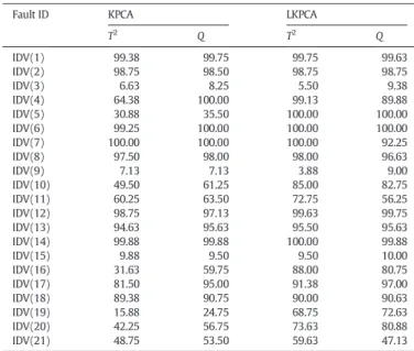
Table 3
Comparison of the fault alarming rates (%) achieved by the KPCA and LKPCA methods.
Fault ID KPCA LKPCA
T2 Q T2 Q IDV(1) 99.38 99.75 99.75 99.63 IDV(2) 98.75 98.50 98.75 98.75 IDV(3) 6.63 8.25 5.50 9.38 IDV(4) 64.38 100.00 99.13 89.88 IDV(5) 30.88 35.50 100.00 100.00 IDV(6) 99.25 100.00 100.00 100.00 IDV(7) 100.00 100.00 100.00 92.25 IDV(8) 97.50 98.00 98.00 96.63 IDV(9) 7.13 7.13 3.88 9.00 IDV(10) 49.50 61.25 85.00 82.75 IDV(11) 60.25 63.50 72.75 56.25 IDV(12) 98.75 97.13 99.63 99.75 IDV(13) 94.63 95.63 95.50 95.63 IDV(14) 99.88 99.88 100.00 99.88 IDV(15) 9.88 9.50 9.50 10.00 IDV(16) 31.63 59.75 88.00 80.75 IDV(17) 81.50 95.00 91.38 97.00 IDV(18) 89.38 90.75 90.00 90.63 IDV(19) 15.88 24.75 68.75 72.63 IDV(20) 42.25 56.75 73.63 80.88 IDV(21) 48.75 53.50 59.63 47.13 Table 4
Comparison of the fault detection time (sample number) achieved by the KPCA and LKPCA methods.
Fault ID KPCA LKPCA
T2 Q T2 Q IDV(1) 167 163 163 166 IDV(2) 171 173 171 175 IDV(3) – – – – IDV(4) 272 161 161 163 IDV(5) 171 161 161 161 IDV(6) 167 161 161 161 IDV(7) 161 161 161 162 IDV(8) 183 177 177 182 IDV(9) 161 – – – IDV(10) 244 208 184 184 IDV(11) 207 167 167 216 IDV(12) 167 163 163 163 IDV(13) 206 197 197 203 IDV(14) 161 162 161 162 IDV(15) 935 – 911 – IDV(16) 356 175 167 169 IDV(17) 189 182 185 182 IDV(18) 249 244 244 244 IDV(19) – – 192 170 IDV(20) 247 245 231 227 IDV(21) 435 409 399 666
Note:–indicates that this fault cannot be detected with the monitoring statistic considered.
0 20 40 60 80 100 T2 Q T2 Q
Average alarming rate (%) 0
20 40 60 80 100
Average alarming rate (%)
KPCA LKPCA KPCA LKPCA
(a)
(b)
Fig. 8.Comparison of the average fault alarming rates achieved by the KPCA and LKPCA schemes: (a) average over Faults IDV(5), IDV(10), IDV(11), IDV(16), IDV(17), IDV(19), IDV(20) and IDV(21), and (b) average over all the 21 fault cases.
0 200 400 600 800 1000 0 2 4 6 Sample Number Q statistic 0 200 400 600 800 1000 0 1 2 3 4 Sample Number T 2 statistic
Fig. 9.On-line monitoring charts of the LKPCA under Fault IDV(4).
0 5 10 15 20 25 30 35 40 45 50 0 10 20 30 Contribution to Q 0 5 10 15 20 25 30 35 40 45 50 0 20 40 60 Variable Number Variable Number Ccontribution to T 2
Fig. 10.Fault identification using the LKPCA-basedT2
andQcontribution plots under Fault IDV(4).
0 100 200 300 400 500 600 700 800 900 1000 35 40 45 50 Sample Number No.51 variable
Fig. 11.The trend of No.51 variable under Fault IDV(4).
0 200 400 600 800 1000 10−1 100 101 102 103 104 105 Sample Number Q statistic 10−1 100 101 102 103 104 105 Q statistic 0 200 400 600 800 1000 Sample Number Fig. 12.On-line monitoring charts of the LKPCA under Fault IDV(6).
0 5 10 15 20 25 30 35 40 45 50 0 500 1000 1500 Variable Number Variable Number Contribution to Q 0 5 10 15 20 25 30 35 40 45 50 0 200 400 600 800 Ccontribution to T 2
Fig. 13.Fault identification using the LKPCA-basedT2
andQcontribution plots under Fault IDV(6).
0 100 200 300 400 500 600 700 800 900 1000 −0.1 0 0.1 0.2 0.3 Sample Number 0 100 200 300 400 500 600 700 800 900 1000 Sample Number No.1 variable 0 50 100 150 No.44 variable
Fig. 14.The trends of No.1 and No.44 variables under Fault IDV(6).
0 200 400 600 800 1000 0 1 2 3 4 Sample Number Q statistic 0 200 400 600 800 1000 0 2 4 6 Sample Number T 2 statistic
0 5 10 15 20 25 30 35 40 45 50 0 20 40 60 Variable Number 0 5 10 15 20 25 30 35 40 45 50 Variable Number Contribution to Q 0 10 20 30 40 Ccontribution to T 2
Fig. 16.Fault identification using the KPCA-basedT2
andQcontribution plots under Fault IDV(4).
0 200 400 600 800 1000 10−1 100 101 102 103 104 10−1 100 101 102 103 Sample Number Q statistic 0 200 400 600 800 1000 Sample Number T 2 statistic
Fig. 17.On-line monitoring charts of the KPCA under Fault IDV(6).
0 5 10 15 20 25 30 35 40 45 50 0 100 200 300 400 Variable Number 0 5 10 15 20 25 30 35 40 45 50 Variable Number Contribution to Q 0 2 4 6 8 Ccontribution to T 2
Fig. 18.Fault identification using the KPCA-basedT2
Afeed. The trends of both the No.1 and No.44 variables are plotted in
Fig. 14. It is clear that the fault identification results correctly reflect the changes of these two variables, which is consistent with the real fault source.
As mentioned in theIntroductionsection, two fault identification methods were proposed in[11,12]for the KPCA based fault diagnosis. The idea presented in[12]is to use variable reconstruction error to iden-tify fault variable, and this method needs the recursive iteration for the reconstructed value of each sample. The method proposed in[11] mea-sures the contribution of each variable using a virtual scale factor meth-od which involves the calculation of a matrix trace for each sample. These two methods are very complex and time-consuming. By contrast, our new contribution plot approach proposed in Subsection 4.2is com-putationally very simple and extremely easy to implement. Moreover, our contribution plot method is very general, and is equally applicable to the KPCA-based scheme. To demonstrate this, we also applied our method to calculate the KPCA-basedT2andQcontribution plots for
fault identification of Faults IDV(4) and IDV(6).
The KPCA-based monitoring charts under Fault IDV(4) are depicted inFig. 15, where it can be seen that the KPCA-basedQ sta-tistic detected this fault at the 161-th sample. Our contribution plot method of Subsection 4.2 was then used to calculate the
KPCA-basedT2andQcontribution plots, which are shown inFig. 16, where
the average contribution value over the 161-th to 165-th samples was used. The KPCA-based monitoring charts under Fault IDV(6) given in
Fig. 17shows that the KPCA-basedQstatistic indicated a fault at the 161-th sample. The KPCA-basedT2andQcontribution plots, averaged
over the 161-th to 165-th samples, were then constructed and shown inFig. 18. The fault identification results ofFigs. 16 and 18are similar to those ofFigs. 10 and 13. More specifically, the quality of the LKPCA-basedT2 contribution plot is slightly better than that of the KPCA-basedT2contribution plot in these two cases. These results confirm
that our contribution plot approach for fault identification is a general one, suitable for both the KPCA and LKPCA.
Although the above simulation results have demonstrated the po-tential of our contribution plot technique in locating fault variables, the power of this technique should not be overstated. For complex fault cases, it is likely that many process variables will be involved and these variables may interact in complicated ways. Therefore, many var-iables may exhibit high contribution values, and it may become difficult to identify real fault variables using the proposed contribution plots. Clearly, further study is warranted to refine the proposed contribution plot approach or to develop alternatives for effectively locating the fault source in complex fault modes.
0 10 20 30 40 50 60 70 80
40 60 80 100
Number of nearest neighbors (K value)
0 10 20 30 40 50 60 70 80
Number of nearest neighbors (K value)
0 10 20 30 40 50 60 70 80
Number of nearest neighbors (K value)
LKPCA Performance (%) 70 80 90 100 110 LKPCA Performance (%) 80 85 90 95 LKPCA Performance (%)
(a) The result under Fault IDV(4)
(b) The result under Fault IDV(5)
(c) The result under Fault IDV(17)
Fig. 19.The LKPCA-based monitoring performance in terms of the average fault alarming rate ofT2
5.3. Selection of K value for adjacency graph
In the LKPCA-based monitoring, the value ofKis an important pa-rameter in determining the weightingswi,jin the optimisation objective
function of local structure analysis. IfKis set to zero or a too small value, the LKPCA optimisation process will not consider the local structure analysis or will consider the local structure of the data set insufficiently. By contrast, ifKis set to a too large value, the LKPCA optimisation pro-cess will over-emphasise the importance of the local structure in the data set. Clearly, there exists an optimal choice ofKvalue, which is prob-lem dependant.
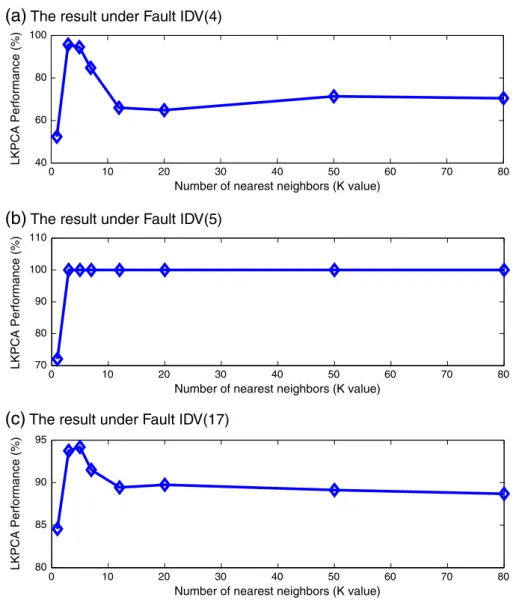
In our simulation study of the TE process, we choseK= 5 empirically. To elaborate further, this value was determined after an experiment of in-vestigating the influence ofKto the LKPCA-based monitoring perfor-mance, in terms of the average fault alarming rate ofT2andQstatistics.
In particular, the value ofKwas set to 1, 3, 5, 7, 12, 20, 50 and 80, and the average fault alarming rates ofT2andQstatistics obtained under
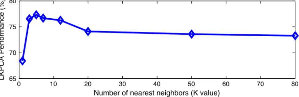
Faults IDV(4), IDV(5) and IDV(17) are shown inFig. 19(a),(b) and (c), respectively. It can be seen that the bestKvalues wereK= 3,K≥3 andK= 5 under Faults IDV(4), IDV(5) and IDV(17), respectively. The average LKPCA-based monitoring performance over all the 21 fault cases was further investigated inFig. 20, where it can be seen that the best choice ofKwasK= 5 on average.
6. Conclusions
A modified kernel principal component analysis, referred to as the LKPCA, has been proposed for process monitoring and fault diagnosis. Our novel contribution has been to integrate the local structure analysis, which is also important for process monitoring and fault diagnosis, into the global optimisation of the standard KPCA technique naturally. Monitoring statistics based on the proposed LKPCA method have been derived for fault detection. Extensive simulation results obtained on the Tennessee Eastman benchmark process have demonstrated that the proposed LKPCA method outperforms the standard KPCA method significantly, in terms of fault detection performance. Furthermore, a contribution plot technique has been developed based on sensitivity analysis of the LKPCA monitoring statistics to identify fault variables. This fault identification technique is computationally very simple and easy to implement, and its potential in locating fault source has been demonstrated in the simulation study. Moreover, the proposed contri-bution plot approach has been shown to be a general method, equally applicable to the standard KPCA based fault diagnosis.
Fault source diagnosis is the most difficult and challenging problem in nonlinear data-driven fault diagnosis, and identifying fault variables in complex fault modes remains an unsolved open problem. Future study is warranted to further enhance the proposed contribution plot approach and to develop more effective fault identification techniques. In particular, it is worth investigating an alternative fault identification approach based on the method of[47,48].
Acknowledgement
This work is supported by the Natural Science Foundation of Shandong Province, China (ZR2011FM014), the Fundamental Research Funds for the Central Universities (10CX04046A), and the National Natural Science Foundation of China (61273160).
References
[1] V. Venkatasubramanian, R. Rengaswamy, S.N. Kavuri, K. Yin, A review of process fault detection and diagnosis Part III: process history based methods, Computers and Chemical Engineering 27 (3) (March 2003) 327–346.
[2] G.A. Cherry, S.J. Qin, Multiblock principal component analysis based on a combined index for semiconductor fault detection and diagnosis, IEEE Transactions on Semi-conductor Manufacturing 19 (2) (May 2006) 159–172.
[3] R. Dunia, S.J. Qin, Joint diagnosis of process and sensor faults using principal compo-nent analysis, Control Engineering Practice 6 (4) (April 1998) 457–469. [4] M.A. Krammer, Nonlinear principal component analysis using autoassociative
neural networks, AICHE Journal 37 (2) (1991) 233–243.
[5] D. Dong, T.J. McAvoy, Nonlinear principal component analysis—based on principal curves and neural networks, Computers and Chemical Engineering 20 (1) (Jan. 1996) 65–78.
[6] H.G. Hiden, M.J. Willis, M.T. Tham, G.A. Montague, Non-linear principal components analysis using genetic programming, Computers and Chemical Engineering 23 (3) (Feb. 1999) 413–425.
[7] Z.-Q. Geng, Q.-X. Zhu, Multiscale nonlinear principal component analysis (NLPCA) and its application for chemical process monitoring, Industrial and Engineering Chemistry Research 44 (10) (2005) 3585–3593.
[8] B. Schölkpof, A.J. Smola, K.-R. Müller, Nonlinear component analysis as a kernel eigenvalue problem, Neural Computation 10 (5) (July 1998) 1299–1319. [9] J.-M. Lee, C.-K. Yoo, S.W. Choi, P.A. Vanrolleghem, I.-B. Lee, Nonlinear process
mon-itoring using kernel principal component analysis, Chemical Engineering Science 59 (1) (Jan. 2004) 223–234.
[10] J.-M. Lee, C.-K. Yoo, I.-B. Lee, Fault detection of batch processes using multiway kernel principal component analysis, Computers and Chemical Engineering 28 (9) (Aug. 2004) 1837–1847.
[11] J.-H. Cho, J.-M. Lee, S.W. Choi, D.-K. Lee, I.-B. Lee, Fault identification for process monitoring using kernel principal component analysis, Chemical Engineering Science 60 (1) (Jan. 2005) 279–288.
[12] S.W. Choi, C.-K. Lee, J.-M. Lee, J.H. Park, I.-B. Lee, Fault detection and identification of nonlinear processes based on kernel PCA, Chemometrics and Intelligent Laboratory Systems 75 (1) (Jan. 2005) 55–67.
[13] X.-G. Deng, X.-M. Tian, Multivariate statistical process monitoring using multi-scale kernel principal component analysis, Proc. 6th IFAC Symp. Fault Detection, Supervi-sion and Safety of Technical Processes (Beijing, China), Aug.29–Sept.1, 2006, 2006, pp. 108–112.
[14] S.W. Choi, J. Morris, I.-B. Lee, Nonlinear multiscale modeling for fault detection and identification, Chemical Engineering Science 63 (8) (April 2008) 2252–2266. [15] Y. Zhang, C. Ma, Fault diagnosis of nonlinear processes using multiscale KPCA and
multiscale KPLS, Chemical Engineering Science 66 (1) (Jan. 2011) 64–72. [16] M. Zvokelj, S. Zupan, I. Prebil, Non-linear multivariate and multiscale monitoring
and signal denoising strategy using kernel principal component analysis combined with ensemble empirical mode decomposition method, Mechanical Systems and Signal Processing 25 (7) (Oct. 2011) 2631–2653.
[17] X.-M. Tian, X.-L. Zhang, X.-G. Deng, S. Chen, Multiway kernel independent component analysis based on feature samples for batch process monitoring, Neurocomputing 72 (7-9) (March 2009) 1584–1596.
[18] P. Cui, J. Li, G. Wang, Improved kernel principal component analysis for fault detec-tion, Expert Systems with Applications 34 (2) (Feb. 2008) 1210–1219.
[19] V.H. Nguyen, J.-C. Golinval, Fault detection based on kernel principal component analysis, Engineering Structures 32 (11) (Nov. 2010) 3683–3691.
[20] M. Jia, F. Chu, F. Wang, W. Wang, On-line batch process monitoring using batch dynamic kernel principal component analysis, Chemometrics and Intelligent Labo-ratory Systems 101 (2) (April 2010) 110–122.
0 10 20 30 40 50 60 70 80
65 70 75 80
Number of nearest neighbors (K value)
LKPCA Performance (%)
Fig. 20.The LKPCA-based monitoring performance in terms of the average fault alarming rate ofT2
[21] Y.-W. Zhang, H. Zhou, S.J. Qin, Decentralized fault diagnosis of large scale processes using multiblock kernel principal component analysis, Act Automatica Sinica 36 (4) (April 2010) 593–597.
[22] I.B. Khediri, M. Limam, C. Weihs, Variable window adaptive kernel principal compo-nent analysis for nonlinear nonstationary process monitoring, Computers and In-dustrial Engineering 61 (3) (Oct. 2011) 437–446.
[23] D.-S. Cao, Y.-Z. Liang, Q.-S. Xu, Q.-N. Hu, L.-X. Zhang, G.-H. Fu, Exploring nonlinear re-lationships in chemical data using kernel-based methods, Chemometrics and Intel-ligent Laboratory Systems 107 (1) (May 2011) 106–115.
[24] G.-H. Fu, D.-S. Cao, Q.-S. Xu, H.-D. Li, Y.-Z. Liang, Combination of kernel PCA and linear support vector machine for modeling a nonlinear relationship between bioactivity and molecular descriptors, Journal of Chemometrics 25 (2) (Feb. 2011) 92–99.
[25] S.T. Roweis, L.K. Saul, Nonlinear dimensionality reduction by locally linear embed-ding, Science 290 (5500) (Dec. 2000) 2323–2326.
[26] M. Belkin, P. Niyogi, Laplacian eigenmaps for dimensional reduction and data repre-sentation, Neural Computation 15 (6) (June 2003) 1373–1396.
[27] X. He, P. Niyogi, Locality preserving projections, in: S. Thrun, L.K. Saul, B. Schölkpf (Eds.), Advances in Neural Information Processing Systems, 16, MIT Press, 2004, pp. 153–160. [28] X. He, D. Cai, W. Min, Statistical and computational analysis of locality preserving
projection, Proc. 22nd Int. Conf. Machine Learning (Bonn, Germany), Aug. 7–11, 2005, 2005, pp. 281–288.
[29] W. Zhang, B. Li, W. Zhou, A LLE-based approach to sensor fault detection, Proc. Int. Joint Conf. Neural Networks (Hong Kong, China), June 1–8, 2008, 2008, pp. 2425–2429. [30] B. Li, Y. Zhang, Supervised locally linear embedding projection (SLLEP) for machinery
fault diagnosis, Mechanical Systems and Signal Processing 25 (8) (Nov. 2011) 3125–3134.
[31] Q. Jiang, M. Jia, J. Hu, F. Xu, Machinery fault diagnosis using supervised manifold learning, Mechanical Systems and Signal Processing 23 (7) (Oct. 2009) 2301–2311. [32] Q. Jiang, M. Jia, J. Hu, F. Xu, Modified Laplacian eigenmap method for fault diagnosis,
Chinese Journal of Mechanical Engineering 21 (3) (2008) 90–93.
[33] K. Hu, J. Yuan, Multivariate statistical process control based on multiway local-ity preserving projections, Journal of Process Control 18 (7–8) (2008) 797–807. [34] J.-D. Shao, G. Rong, J.M. Lee, Generalized orthogonal locality preserving projections for nonlinear fault detection and diagnosis, Chemometrics and Intelligent Laboratory Systems 96 (1) (March 2009) 75–83.
[35] J.-B. Yu, Bearing performance degradation assessment using locality pre-serving projections, Expert Systems with Applications 38 (6) (June 2011) 7440–7450.
[36] J.-B. Yu, Bearing performance degradation assessment using locality preserving projections and Gaussian mixture models, Mechanical Systems and Signal Process-ing 25 (7) (Oct. 2011) 257–2588.
[37] M. Zhang, Z. Ge, Z. Song, R. Fu, Global–local structure analysis model and its application for fault detection and identification, Industrial and Engineering Chemistry Research 50 (11) (April 2011) 6837–6848.
[38] J.-M. Lee, C.K. Yoo, I.-B. Lee, Statistical process monitoring with independent compo-nent analysis, Journal of Process Control 14 (5) (Aug. 2004) 467–485.
[39] E. Parzen, On estimation of a probability density function and mode, Annals of Mathematical Statistics 33 (3) (Sept. 1962) 1066–1076.
[40] B.W. Silverman, Density Estimation, Chapman & Hall, London, 1996.
[41] L.H. Chiang, E.L. Russell, R.D. Braatz, Fault Detection and Diagnosis in Industrial Systems, Springer-Verlag, London, 2001.
[42] J.A. Westerhuis, S.P. Gurden, A.K. Smilde, Generalized contribution plots in multivar-iate statistical process monitoring, Chemometrics and Intelligent Laboratory Systems 51 (1) (May 2000) 95–114.
[43] L. Petzold, S. Li, Y. Cao, R. Serban, Sensitivity analysis of differential-algebraic equations and partial differential equations, Computers and Chemical Engineering 30 (10–12) (Sept. 2006) 1553–1559.
[44] J.J. Downs, E.F. Vogel, A plant-wide industrial process control problem, Computers and Chemical Engineering 17 (3) (March 1993) 245–255.
[45] N. Lu, F. Wang, F. Gao, Combination method of principal component and wave-let analysis for multivariate process monitoring and fault diagnosis, Industrial and Engineering Chemistry Research 42 (18) (July 2003) 4198–4207. [46] J. Lee, B. Kang, S.-H. Kang, Integrating independent component analysis and local
outlier factor for plant-wide process monitoring, Journal of Process Control 21 (7) (July 2011) 1011–1021.
[47] G.J. Postma, P.W.T. Krooshof, L.M.C. Buydens, Opening the kernel of kernel partial least squares and support vector machines, Analytica Chimica Acta 705 (1–2) (Oct. 2011) 123–134.
[48] P.W.T. Krooshof, B. Ustün, G.J. Postma, L.M.C. Buydens, Visualization and recovery of the (bio)chemical interesting variables in data analysis with support vector machine classification, Analytical Chemistry 82 (16) (Aug. 2010) 7000–7007.