econ
stor
www.econstor.eu
Der Open-Access-Publikationsserver der ZBW – Leibniz-Informationszentrum Wirtschaft
The Open Access Publication Server of the ZBW – Leibniz Information Centre for Economics
Nutzungsbedingungen:
Die ZBW räumt Ihnen als Nutzerin/Nutzer das unentgeltliche, räumlich unbeschränkte und zeitlich auf die Dauer des Schutzrechts beschränkte einfache Recht ein, das ausgewählte Werk im Rahmen der unter
→ http://www.econstor.eu/dspace/Nutzungsbedingungen nachzulesenden vollständigen Nutzungsbedingungen zu vervielfältigen, mit denen die Nutzerin/der Nutzer sich durch die erste Nutzung einverstanden erklärt.
Terms of use:
The ZBW grants you, the user, the non-exclusive right to use the selected work free of charge, territorially unrestricted and within the time limit of the term of the property rights according to the terms specified at
→ http://www.econstor.eu/dspace/Nutzungsbedingungen By the first use of the selected work the user agrees and declares to comply with these terms of use.
zbw
Leibniz-Informationszentrum WirtschaftJung, Robert; Liesenfeld, Roman; Richard, Jean-François
Working Paper
Dynamic Factor Models for Multivariate Count Data:
An Application to Stock-Market Trading Activity
Economics working paper / Christian-Albrechts-Universität Kiel, Department of Economics, No. 2008,12
Provided in cooperation with:
Christian-Albrechts-Universität Kiel (CAU)
Suggested citation: Jung, Robert; Liesenfeld, Roman; Richard, Jean-François (2008) : Dynamic Factor Models for Multivariate Count Data: An Application to Stock-Market Trading Activity, Economics working paper / Christian-Albrechts-Universität Kiel, Department of Economics, No. 2008,12, http://hdl.handle.net/10419/22056
Dynamic Factor Models for
Multivariate Count Data: An Application
to Stock-Market Trading Activity
by Robert C. Jung, Roman Liesenfeld and Jean-François Richard
No 2008-12
Economics Working Paper
Dynamic Factor Models for Multivariate Count Data: An
Application to Stock-Market Trading Activity
Robert C. Jung
Universität Erfurt, Department of Economics, Germany Roman Liesenfeld∗
Christian-Albrechts-Universität Kiel, Department of Economics, Germany Jean-François Richard
University of Pittsburgh, Department of Economics, USA (July 22, 2008)
Abstract
We propose a dynamic factor model for the analysis of multivariate time series count data. Our model allows for idiosyncratic as well as common serially correlated latent factors in order to account for potentially complex dynamic interdependence between series of counts. The model is estimated under alternative count distributions (Poisson and negative binomial). Maximum Likelihood estimation requires highdimensional numerical integration in order to marginalize the joint distribution with respect to the unobserved dynamic factors. We rely upon the Monte Carlo integration procedure known as Ecient Importance Sampling which produces fast and numerically accurate estimates of the likelihood function. The model is applied to time series data consisting of numbers of trades in 5 minutes intervals for ve NYSE stocks from two industrial sectors. The estimated model accounts for all key dynamic and distributional features of the data. We nd strong evidence of a common factor which we interpret as reecting marketwide news. In contrast, sectorspecic factors are found to be statistically insignicant.
Keywords: Dynamic latent variables, Importance sampling, Mixture of distribution models, Poisson distribution, Simulated Maximum Likelihood;
∗Corresponding author. Tel.: +49-431-8803810; fax: +49-431-8807605. E-mail address:
1. Introduction
Modelling of dispersion and serial correlation for univariate count series has received much attention over recent years. Existing approaches can be broadly classied as either observation or parameter driven. The monographs of Kedem and Fokianos (2002) and McKenzie (2003) provide excellent overviews. More recent contributions include Jung et al. (2006), Neal and Subba Rao (2007) and Jung and Tremayne (2008).
Multivariate dynamic models for count data remain few. As discussed by Cameron and Trivedi (1998, Section 8.1), this might be explained by the fact that classical inference in multivariate count data models has proven to be analytically as well as computationally very demanding. This is par-ticularly relevant for models attempting to capture the complex correlation structure characterizing many multivariate count time series. Three pioneering multivariate applications are found in Jør-gensen et al. (1999), Held et al. (2005), and Heinen and Rengifo (2007). The specication proposed by Jørgensen et al. (1999) belongs to the class of parameterdriven models. It is a multivariate Poisson statespace model with a common factor following a gamma Markov process. These specic distributional assumptions produce a model which can be analyzed by a Kalman lter. The model is used to assess the impact of air pollution on daily emergency admission counts in an hospital for four sickness categories. Held et al. (2005) propose an observationdriven multivariate model which imposes a simple vectorautoregressive structure for the means. This model can be estimated by standard Maximum Likelihood (ML). It is applied to infectious disease surveillance counts from a measle epidemic. Heinen and Rengifo (2007) also adopt an observationdriven approach extending the univariate autoregressive conditional Poisson model of Heinen (2003). A copula approach is used to represent contemporaneous correlations among time series counts. Since ecient joint ML estima-tion is not feasible, the authors rely upon a consistent though less ecient twostage ML approach for separate estimation of the parameters of the marginal distributions and those of the copula. Their model is then used to analyze comovements in the number of trades for stocks traded at the New York Stock Exchange (NYSE). Other multivariate count models rely upon panel data techniques, with emphasis on unobserved heterogeneity in the individual series. See Winkelmann (2008) for a recent survey.
In the present paper we adopt a parameterdriven approach and propose a new exible, parsi-monious and easy to interpret dynamic factor model for multivariate count series. It builds upon and generalizes earlier models by Jørgensen et al. (1999) and Wedel et al. (2003). The former model includes a single dynamic common factor only and no dynamic idiosyncratic components. The latter model is a static multivariate Poisson factor model for cross-sectional analyses. Our model allows for serially correlated common as well as idiosyncratic factors driving the conditional means of the count distributions. Therefore, it can represent nontrivial contemporaneous and temporal interactions across count series. It can also accommodate dierent distributional assumptions for the conditional distribution of the counts given the factors. This can be critical since the commonly used Poisson distribution has an index of dispersion equal to one (the latter being dened as the ratio between the variance and the mean). However, count data often exhibit strong overdispersion (index signi-cantly larger than one) which can not be fully captured by a conditional Poisson distribution even if a varying conditional mean generates by itself an overdispersed unconditional distribution. Hence, it is important to allow for conditional distributions which can accommodate overdispersion, such as the negative binomial (here after Negbin) and the double Poisson.
Our model depends nonlinearly upon its dynamic latent factors. Whence, likelihood evaluation requires highdimensional numerical integration, for which we use the Ecient Importance Sampling (hereafter EIS) procedure developed by Richard and Zhang (2007). EIS is a generic, exible and easy to implement Monte Carlo integration procedure specically designed to maximize numerical accuracy. It also facilitates exploring alternative model specications which typically require only minor modications of a baseline EIS implementation. Last but not least, EIS can be used to compute ltered and/or smoothed estimates of the latent factors themselves. Several diagnostic test statistics are based upon such estimates.
Our model is then applied to a multivariate time series consisting of numbers of trades in 5minutes intervals for ve stocks traded at the NYSE. We implicitly adopt the information ow interpretation associated with the mixture-of-distribution model of Tauchen and Pitts (1983). See also Andersen (1996) and Liesenfeld (2001). In this context, numbers of trades are directly inuenced by the arrival of new information, whether specic to a single stock (idiosyncratic factor), to an industry (sector
factor), or to the market (market factor).
The paper is organized as follows. The multivariate dynamic factor model is introduced in Section 2, Section 3 discusses ML estimation, ltering and smoothing based upon EIS. The application to NYSE data is presented in Section 4. Section 5 concludes. Technical derivations are regrouped in an Appendix.
2. Dynamic Factor Model for Multivariate Count Data
The econometric model we propose consists of a dynamic extension of the static multivariate Poisson factor model introduced by Wedel et al. (2003). Consider a Jdimensional vector of counts yt =
(yt1, ..., ytJ)0 recorded at time t, (t= 1, ..., T). Dynamics will be introduced at the level of the latent factors. Whence, counts are assumed to be conditionally independently distributed with Poisson distributions p(ytj|θtj) = exp(−θtj)θ ytj tj ytj! , t= 1, .., T, j= 1, ..., J, (1)
whose meansθtj are latent random variables. We assume the existence of a link functionb(·), whereby the mean vector θt = (θt1, ..., θtJ)0 can be expressed as a linear function of a Pdimensional vector of latent random factorsft, say
b(θt) =µ+ Γft, (2)
where µ denotes a vector of xed intercepts and Γ a (J ×P) matrix of factor loadings. The P
latent factors in ft are assumed to be independent of each other. A log-link functionb(θt) = ln(θt) is convenient since it implies positivity of θt without parametric restrictions on (µ,Γ). Alternative link functions will not be considered here.
In the context of our NYSE application considering the joint behavior of the number of trades for dierent stocks, we allow for a single common market factorλt, S < J industryspecic factors τt = (τt1, ..., τtS)0, and J stockspecic factors ωt = (ωt1, ..., ωtJ)0. Whence, ft is partitioned into
ft= (λt, τt0, ωt0)0 and P =J +S+ 1. The matrix of factor loadings is partitioned conformably with
ftintoΓ = (Γλ,Γτ,Γω), whereΓλ = (γjλ) is aJdimensional vector, Γτ = (γjτs)aJ×S matrix with
matrix. Whence, the log-mean function for stockj, belonging to industry sis given by lnθtj =µj+γjλλt+γ τsj j τtsj+γ ωj j ωtj, (3)
where the index sj denotes the industry of rm j.
In order to account for possible serial and cross-correlation in the counts, we assume that the factors follow independent gaussian AR(1) processes, say
λt|λt−1 ∼ N(κλ+δλλt−1 , [νλ]2) (4) τts|τt−1s ∼ N(κτs+δτsτt−1s, [ντs]2), (5)
ωtj|ωt−1j ∼ N(κωj+δωjωt−1j , [νωj]2). (6) To ensure stationarity of the factors, it is assumed that |δλ| < 1, |δτs| < 1, and |δωj| < 1. Other distributional and dynamic specications for the factors are easily accommodated. Under an identity linkb(·), for example, a Gamma transition distribution or a log-normal transition distribution would
be suitable factor specications (see, Jørgensen et al., 1999, and Jung and Liesenfeld, 2001).
The model as specied is unidentied. Identication for the static case with i.i.d. factors is discussed in Wedel et al. (2003) and can be extended to the dynamic model introduced here. We impose the restrictions thatκλ =κτs =κωj = 0for s= 1, ..., S and j = 1, ..., J in order to identify the µj's (see Equations 46). Furthermore, we set γ1λ = 1, γ
ωj
j = 1 for j = 1, ..., J, and γ τs
j = 1
for one arbitrarily selected stock j in industry s for s = 1, ..., S (see Equation 3). This eliminates
indeterminacies in the factor scales.
Under the assumed Poisson distribution, whose dispersion index equals one, overdispersion of the counts can only originate from the unconditional variances of the factors, which themselves critically depend on the persistence parameters(δλ, δτs, δωj). In order to relax this close relationship between overdispersion and persistence, we can substitute a more exible distribution for the Poisson. One
such distribution which we shall apply below is the negative binomial (Negbin), which is given by p(ytj|θtj) = Γ(ytj+ 1/σ2j) Γ(1/σj2)Γ(ytj+ 1) 1 1 +σj2θtj !1/σ2j θtj θtj+ 1/σj2 !ytj , (7)
whereΓ(·) denotes the Gamma function. Its mean and variance are given by θtj and θtj(1 +σj2θtj), respectively. The overdispersion is a monotone increasing function of σj > 0 and the Poisson distribution in Equation (1) obtains as the limit for σj → 0. The double Poisson distribution proposed by Efron (1994) or the generalized Poisson distribution proposed by Consul (1989) oer alternatives to capture (conditional) overdispersion but will not be considered here.
3. EIS Based Inference
3.1 EIS
The evaluation of the likelihood function for the model described by Equations (1) to (6) requires integrating the joint density of counts and factors with respect to the T ·P latent factor variables
(in our application below T·P ranges from 22,875 to 36,600!). For likelihood evaluation counts are
kept xed at their observed values and are, therefore, omitted from notation except for the fact that densities need to be time indexed to reect their dependence on the data.
The likelihood integral to be evaluated is of the following form:
L(ψ) = Z · · · Z T Y t=1 ϕt(ft, ft−1;ψ)dfT· · ·df1, (8)
whereψregroups the parameters of the model. ϕt denotes the product of the timet densities foryt givenftand forftgiven ft−1 as dened by Equations (1) to (6). The initial condition f0 is assumed
to be a known constant, which we set in our application tof0 =E(ft) = 0. If all relevant integrals had analytical solutions, L(ψ) would obtain from the following (backward) recursive sequence of
Pdimensional integrals
L (f− ;ψ) =
Z
withLT+1(fT;ψ)≡1, andL(ψ)≡L1(f0;ψ). When these integrals are analytically intractable, EIS,
as proposed by Richard and Zhang (2007), essentially amounts to constructing a sequence of auxiliary parametric density kernels {kt(ft, ft−1;at), at ∈ At}Tt=1, which (i) are analytically integrable in ft given ft−1, and (ii) are amenable to MC simulation. The corresponding importance samplers are
then given by mt(ft|ft−1;at) = kt(ft, ft−1;at) χt(ft−1;at) , with χt(ft−1;at) = Z kt(ft, ft−1;at)dft. (10) The integral in Equation (8) is then rewritten as
L(ψ) =χ1(f0;a1) Z · · · Z T Y t=1 ϕt(ft, ft−1;ψ)χt+1(ft;at+1) kt(ft, ft−1;at) mt(ft|ft−1;at)dfT · · ·df1, (11)
withχT+1(·)≡1. Hereχt+1 essentially substitutes for the analytically intractableLt+1 in Equation
(9). EIS then aims at selecting {ˆat}Tt=1 which minimizes the MC sampling variances of the ratios ϕt ·χt+1/kt as functions of ft and ft−1, not just ft. An MC-EIS approximate solution of this
minimization problem obtains from the following backward sequence of auxiliary Least Squares (LS) problems: (ˆct,ˆat) = arg min ct∈R,at∈At N X i=1 ( lnhϕt f˜t(i),f˜ (i) t−1;ψ ·χt+1 f˜t(i); ˆat+1 i (12) −ct−lnkt f˜t(i),f˜ (i) t−1;at )2 , where {f˜t(i)}T
t=1 denotes a trajectory drawn from the (forward) sequence of auxiliary samplers
{mt(ft|f˜t(−i)1; ˆat)}Tt=1 with i = 1, ..., N (i.i.d.). In order to account for the fact that the {f˜ (i)
t } in Equation (12) also depends on{ˆat}, the latter obtains as xed-point solutions of the following iter-ated sequences of auxiliary backward LS problems:
· · · → {ˆa(tk−1)}Tt=1 → forward draws :{{ ˜ ft(i),(k−1)}Tt=1}Ni=1} → backward LS :{ˆa (k) t }Tt=1 → · · · .
At convergence the EIS estimate ofL(ψ) is given by: ¯ LN(ψ) =χ1(f0; ˆa1) 1 N N X i=1 T Y t=1 " ϕt( ˜ft(i),f˜ (i) t−1;ψ)χt+1( ˜ft(i); ˆat+1) kt( ˜ft(i),f˜ (i) t−1; ˆat) # . (13)
For smooth convergence of the EIS xed-point sequence as well as subsequent continuity of L¯N(ψ)
w.r.t.ψ, it is critical that alli-th trajectories{f˜t(i),(k)}T
t=1 be obtained by transforming a single set of
Common Random Numbers (CRNs), say{u˜(ti)}T
t=1. CRNs are N(0,1)for gaussian EIS samplers and U(0,1)for EIS-sampling densities simulated by cdf inversion. Most importantly, EIS-density kernels
within the exponential family of distributions are linear in the auxiliary parameters at under their natural parametrization as well as closed under multiplication. As detailed in the Appendix, these two properties considerably simplify the application of EIS to our model. Note nally that {ˆat}Tt=1
is an implicit function ofψ. Therefore, maximal numerical eciency requires complete reruns of the
EIS algorithm for any new value ofψ. See Richard and Zhang (2007) for details.
3.2 EIS likelihood for the dynamic count data model
EIS estimation of the likelihood function of the model dened by Equations (1) to (6) turns out to be conceptually straightforward and numerically accurate though notationally tedious. In this section we only outline the EIS implementation. All relevant algebraic details are regrouped in the Appendix.
Under the loglink function, the Poisson density in Equation (1) is rewritten as
p(ytj |φtj) =
exp ytjφtj−eφtj
ytj!
, (14)
withφtj= lnθtj. Equations (2) and (3) are rewritten in matrix form as
withφ0t= (φt1, . . . φtJ), ft0= (λt, τt1, . . . τtS, ωt1, . . . , ωtJ,), and Γ = γ1λ γ2λ ... γJλ γτ1 0 . . . 0 0 γτ2 . . . 0 ... ... ... 0 0 γτS γω1 1 0 . . . 0 0 γω2 2 . . . 0 ... ... ... 0 0 γωJ J , (16) whereγτs = (γτsj
j ), for j=Js+ 1, . . . , Js+1 (J1= 0,JS+1=J) denotes the vector of factor loadings on the industry factor τts for all stocks which belong to sector s. Equations (4) to (6) imply that
p(ft|ft−1)∼N ∆ft−1, H−1
, (17)
where ∆ and H are both diagonal and H denotes the inverse of the covariance matrix of ft given
ft−1.
In order to apply sequential EIS to this model, we rst note that the factorϕt(ft, ft−1;ψ) in the
likelihood integral (8) and (11) is given by
ϕt(ft, ft−1;ψ) =p(ft|ft−1)· J Y j=1 p(ytj |φtj) , (18)
wherep(ft|ft−1)is linear gaussian andφtjis a linear function offt. Next, note that ifkt(ft, ft−1;at) is a gaussian kernel in bothft and ft−1, then its integrating constant w.r.t. ft given byχt(ft−1;at) is a gaussian kernel inft−1. By recursion this implies that the sole nongaussian term in the product ϕtχt+1 to be approximated bykt is the product of theJ densitiesp(ytj |φtj). It follows that all we have to do is to construct gaussian approximates in φtj to the latter densities in order to produce a gaussian kernel kt for (ft, ft−1). The kernel kt then consists of the product of p(ft|ft−1) by J
univariate gaussian kernels in the φtj's and by χt+1. Moreover, the factors p(ft|ft−1) and χt+1
appear in logs on both sides of the auxiliary EIS regressions in Equation (12) and cancel out. All in all, the EIS auxiliary regression for the approximation of ϕtχt+1 byktsimplies into J independent bivariate linear LS regressions of {lnp(ytj | φ˜tj(i))}Ni=1 on {( ˜φ
(i)
tj , [ ˜φ
(i)
auxiliary regressions run fast and produce numerically very accurate evaluations of the likelihood function, rendering ML-EIS estimation of the model fully operational.
The corresponding matrix algebra, which essentially consists of regrouping three gaussian kernels in (ft, ft−1) and integrating out ft, is conceptually straightforward. Details are regrouped in the
Appendix.
Last but not least, note that if we replace the Poisson density by the Negbin density in Equation (7), we only need to modify accordingly the dependent variables in the auxiliary EIS regressions, a trivial adjustment all together.
3.3 Filtering and smoothing
In many state-space applications such as the one analyzed here, interest lies also in the estimation of the latent states (i.e. in our application the factors) whether for diagnostic checking, interpreta-tion and/or forecasting. Since, however, factors are one-time occurrences (incidental in statistical jargon) they obviously cannot be consistently estimated. Nevertheless, their moments conditional upon alternative information sets are functions of the parameters of the model and can therefore be consistently estimated.
The ltered moments offtare dened as being conditional upon information available up to time
t−1denoted byYt−1. In the present paper we shall compute means and variances ofexp(γj0ft), where
γj0 denotes thejth row ofΓ. These moments are instrumental in the computation of the standardized
Pearson residuals
ztj = ytj−E(ytj|Yt−1)
Var(ytj|Yt−1)1/2
. (19)
These residuals are critical components of a variety of diagnostic statistics since they should have zero mean and unit variance and should be serially uncorrelated if the model is correctly specied. Under the Poisson model the relevant conditional moments ofytj are given by
and
Var(ytj|Yt−1) = exp{µj} ·E(exp{γ0jft}|Yt−1) + exp{2µj} ·Var(exp{γj0ft}|Yt−1), (21)
respectively. The ltered moments ofexp(γj0ft) take the form of ratios of integrals in{fr}tr=1 which
are functionally similar to the likelihood integral in Equation (8) with products running only up to period t−1. Both numerator and denominator can be accurately approximated by EIS. Moreover,
both EIS approximations should use the same set of CRNs in order to induce positive correlation between numerator and denominator, resulting in additional eciency gains.
Smoothed moments of ft are dened as being conditional on the entire sample YT and are also computed by EIS (and are typically very close to the moments of the EIS samplers since the latter can be interpreted as approximations of the posterior densities of the factors). Smoothed moments provide, therefore, an ex-post image of the factor history over the sample period.
4. Application to Stock-Market Trading Volume
4.1 The data
Dierent versions of the dynamic factor model introduced in Section 2 are applied to the number of trades in 5-minute intervals between 9:45 AM and 4:00 PM for J = 5 stocks traded at the
NYSE: Two companies - P.H. Glatfelter Company (GLT) and Wausau Paper Corporation (WPP) belong to the industry subsector paper; three companies Empire District Electric Company (EDE), Northeast Utilities (NU) and Westar Energy, Inc. (WR) belong to the industry subsector conventional electricity. Data are taken from the TAQ (Trades and Quotes) data set, provided by the NYSE. The time period covered is the rst quarter of 2005 (January 3, 2005 March 31, 2005) with 61 trading days. As there are 75 5-minute intervals per day, the sample size isT = 4575. See the top
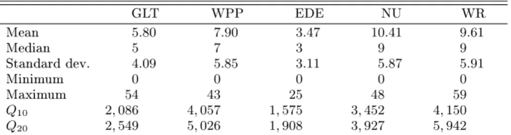
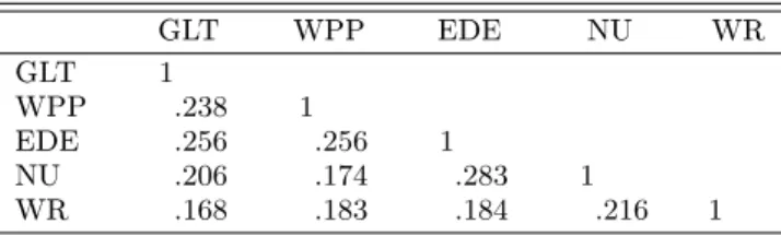
panel of Figure 3 for time series plots of the number of trades. Descriptive statistics are provided in Table 1, and Table 2 reports the sample correlations across the ve stocks. As one can see, the empirical distribution of the number of trades is clearly overdispersed. The LjungBox statistics for the number of trades Q10 and Q20 including 10 and 20 lags, respectively, indicate strong serial
ve stocks are all positive.
4.2 Daily trading pattern
It is wellknown that daily trading activity has a distinctive U-shape pattern (see, e.g., Admati and Peiderer, 1988). In order to capture it we introduce a Fourier series for the intercept of the logmean function (see Equation 3). Specically,µj is replaced by a cyclical termµtj dened as
µtj =µj+α0jxt, (22)
with α0j = (α1j, . . . , α4j) and x0t = (cos(2πt/75),sin(2πt/75),cos(4πt/75),sin(4πt/75)), accounting for the fact that there are 75 5-minutes intervals in a trading day. EIS trivially accommodates this extension. The ltering equations (20) and (21) are modied as follows:
E(ytj|Yt−1, xt) = exp{µj+α0jxt} ·E(exp{γj0ft}|Yt−1, xt), (23)
Var(ytj|Yt−1, xt) = exp{µj +αj0xt} ·E(exp{γj0ft}|Yt−1, xt) (24)
+ exp{2(µj+α0jxt)} ·Var(exp{γj0ft}|Yt−1, xt).
4.3 Univariate Analysis
As initial step, we rst estimate a univariate dynamic Poisson model for each of the ve stocks separately. This model is dened by Equations (1) and (6) withκωj = 0 together with
lnθtj =µtj+ωtj, (25)
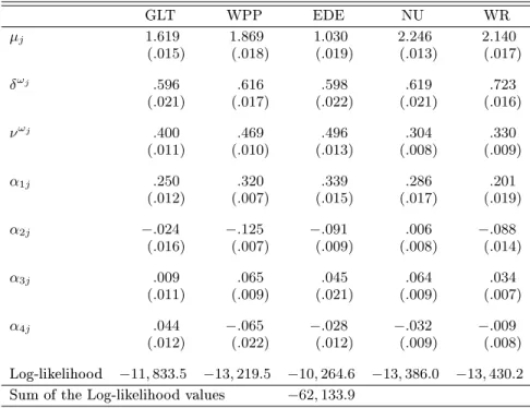
and Equation (22). This univariate (parameterdriven) dynamic Poisson model was introduced by Zeger (1988) and analyzed by Chan and Ledolter (1995), Kuk and Cheng (1997), Jung and Liesenfeld (2001), and Jung et al. (2006). The ML-EIS estimation results based on a MC sample size of N = 50are found in Table 3. Most importantly, we nd that the parameters governing the
stochastic latent processes {ωtj}5j=1 and those characterizing the diurnal patterns are quite similar
across the ve stocks. In particular, estimates of δωj range from 0.60 to 0.72 and are indicative of strong persistence, while the estimates ofνωj range from 0.30 to 0.50. These ndings motivate our subsequent multivariate analysis where we shall aim at identifying common factors. They also allow us to impose in Equation (22) a common diurnal pattern to the ve stocks obtained by setting the vectors α0j = α0 = (α1, . . . , α4) for j = 1, ..., J , thereby preserving parsimony in the multivariate
specication.
4.4 Multivariate Factor Models
4.4.1 Poisson Model with one common factor
Allowing for a single common factor λt in addition to the idiosyncratic factors ωtj, the log-mean function in the conditional Poisson distribution (1) for stockj is now given by
lnθtj=µtj+γjλλt+ωtj, (26)
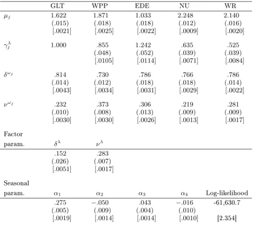
withγ1λ = 1, together with Equations (4), (6) and (22) under the restriction αj =α. Joint ML-EIS estimates based upon N = 50 trajectories are found in Table 4. ML-EIS estimation requires
approximately 65 BFGS iterations and takes of the order of 100 minutes on a Core 2 Duo Intel 2.7 GHz processor using GAUSS on Windows XP. (We also experimented with the Nelder-Mead simplex method for maximizing the log-likelihood functions (see, e.g., Press et al., 1988). It turned out that it produces the same results and requires about the same computing time as the BFGS algorithm. However, for higher dimensional factor models and/or less well-behaved likelihood functions we advise the use of this gradient free simplex algorithm.) MC numerical standard deviations of the EIS parameter estimates used as measures of numerical precision are obtained from 20 i.i.d. ML-EIS estimations conducted under dierent CRN seeds (see Richard and Zhang, 2007 for details). They indicate that the parameter estimates are numerically very accurate. The fact that such high accuracy obtains with as little as N = 50 trajectories indicates that the likelihood integrands
accurately approximated by the EIS-sampler (using 54,900 auxiliary parameters). In particular, the
R2s of the EIS auxiliary LS-problems (12) are typically larger than 0.99.
All parameter estimates are reasonable and apart fromα4 signicant at the 1% signicance level.
The estimates of the parameters for the common processδλ and νλ indicate a substantial variation
and a slight, yet signicant, persistence. The estimates of the factor loadings ranging from 0.53 to 1.24 suggest that the trading activity of all stocks load signicantly on the common factor, which is not surprising as trading is positively correlated across stocks. The estimates of the parameters characterizing the idiosyncratic factors indicate substantially more persistence than for the common factor as well as uniformly more persistence than their univariate counterparts in Table 3. Hence, the idiosyncratic factors capture the persistent movements of the trading process, whilst the common factor accounts for the more transitory variation. Note, furthermore, that the estimatedα-parameters
governing the deterministic seasonal eects are similar in magnitude to those obtained under the univariate models (see Table 3). Figure 1 shows the estimated diurnal seasonal eects for the number of trades obtained under the dynamic factor model. They exhibit the well-documented U-shape
pattern. The sum of the individual log-likelihood values for the ve independent univariate models equals -62,134 (see Table 3) which is substantially smaller than the log-likelihood value of -61,631 for the multivariate factor model. This large dierence reects the fact that, as shown below, the common factor model fully accounts for observed correlations between trading activities, in sharp contrast with the univariate models which ignore them.
In order to assess the reliability and the statistical properties of the ML-EIS estimator in this multivariate factor model we conducted a small simulation experiment, in which we drew 20 ctitious samples of size 4575 from that model setting the parameters equal to their estimates obtained from the real data. MC mean and standard deviation of the ML-EIS estimates obtained for the ctitious samples are provided in Table 5 and indicate that the ML-EIS estimation procedure is statistically very well behaved. Figure 2 shows the time series of the true log conditional mean lnθtj of the rst count data series for the rst 500 time periods together with its smoothed estimates E(lnθtj|Y) obtained for simulated data. Unsurprisingly, the series of smoothed estimates closely follows the true value.
The parameter estimates in Table 4 can be used to compute the implied estimates of the means and the covariance of the unconditional distribution for the number of trades, to be compared with their sample counterparts. In the presence of deterministic diurnal eects, the unconditional means and variances for the trades of stockj under the factor model are
E(ytj) =ET exp{µtj+ 0.5γj0Σfγj}
(27) and
Var(ytj) = VarT exp{µtj+ 0.5γj0Σfγj}
(28) +ET exp{2µtj+γj0Σfγj} exp{γj0Σfγj} −1 + exp{µtj+ 0.5γj0Σfγj} ,
where γj represents the vector of the factor loadings for stock j and Σf the covariance matrix of the vector of factorsft. The notation ET and VarT indicate sample mean and sample variance com-puted w.r.t. the deterministic variation of the diurnal seasonal eects. The corresponding covariance between trading of stockj and stock k is obtained from the cross moments
E(ytjytk) =ET exp{µtj+µtk+ 0.5(γj+γk)0Σf(γj +γk)}
, j6=k. (29)
The estimates of the unconditional mean and covariance matrix of ytare given by
ˆ E(yt) = 5.83 7.93 3.45 10.41 9.72 and Varˆ (yt) = 16.93 5.46 38.70 3.11 3.76 9.55 5.94 7.40 4.02 33.11 4.99 6.27 3.34 7.19 39.07 ,
respectively. The corresponding sample moments are given by ¯ y= 5.80 7.90 3.47 10.41 9.61 and Σy¯= 16.75 5.68 34.17 3.26 4.65 9.65 4.95 5.97 5.17 34.41 4.09 6.32 3.37 7.47 34.89 ,
respectively. The close match between those two sets of moments indicates that the common factor model provides an excellent parsimonious representation of the contemporaneous correlation across the ve stocks.
In order to assess the relative importance of the common factor, idiosyncratic factors and the diurnal component we computed their relative contribution to the overall variance of the log-link function for the individual stockslnθtj. The implied estimates of the contributions to the variation
of the log-link function are reported in the upper panel of Table 8. The fraction of variation explained by the common factor varies between 8% (WR) and 31% (EDE) while that of the idiosyncratic factors range between 56% (GLT) and 76% (WR). Even though the idiosyncratic factors explain a larger fraction of variation inlnθtj than the common factor, it is important to remember that the latter is indispensable to capture observed contemporaneous correlations.
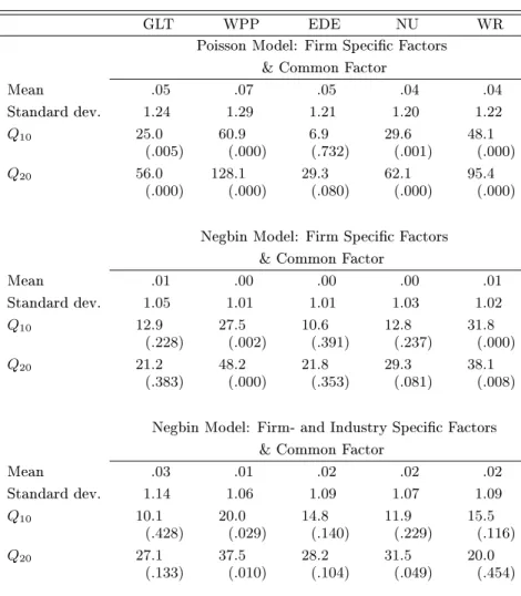
For diagnostic checking we computed the standardized Pearson residuals ztj as dened by Equa-tions (19), (23) and (24). The conditional moments of exp{γj0ft} appearing in the Equations (23) and (24) are ltered moments and are evaluated by EIS as described in Section 3.3 above. The upper panel of Table 9 summarizes the properties of the Pearson residuals. Their sample means are all close to zeros. However, their standard deviations are all substantially larger than 1. This indicates that there is more variation and overdispersion in the data than the model accounts for. Furthermore, the Ljung-Box statistics for the residuals including 10 and 20 lags indicates that the model does not fully capture the dynamic behavior of the trading activity even though it dramatically reduces the Ljung-Box statistic for the raw data as given in Table 1. The bottom row of Figure 3 displays the time series of the standardized residuals for the 5 stocks. The comparison with the time series plot
of the raw data (see top row of Figure 3) reveals that the model accounts for a substantial fraction of the variation in the data.
4.4.2 Negbin Model with one common factor
In order to better account for overdispersion and to allow for more exibility to capture the serial correlation we replace the conditional Poisson density in Equation (1) by the more exible Negbin density in Equation (7). As explained in Section 3.2 above, this substitution only requires minor modications of the baseline EIS-ML algorithm.
The results of the ML-EIS estimation of the Negbin factor model with one common and J
id-iosyncratic factors are reported in Table 6. Note that the substitution of the Negbin for the Poisson distribution increases the value of the maximized likelihood function by 381, indicative of a much better t. Moreover, the additionalσ-parameters measuring the deviation from the Poisson
distribu-tion are in each case statistically signicantly larger than zero at any convendistribu-tional signicance level. On the other hand the estimates of the intercept parameters (µj), the factor loadings (γλj), and of the
seasonal parameters (αi) obtained under the Poisson and the Negbin specication are very similar to each other, indicating a fairly robust factor structure. Note, however, that theδ-coecients have
increased under the Negbin model while the ν-parameters have decreased. This indicates that the
factors, whether common or idiosyncratic evolve more smoothly over time and with greater persis-tence under the Negbin. These dierences also suggest that a substantial part of the variation in trading activities, which was attributed to persistent shocks in the factor processes under the Poisson model, is now interpreted as transitory and attributed to conditional overdispersion (σj >0) under the Negbin model. (Such a substitution eect can also be observed for applications of the stochastic volatility models when the usual gaussian density for the conditional distribution of the returns is, in the presence of outliers, substituted by a fat-tailed student-t assumption, see, e.g., Liesenfeld and Jung, 2000). Note also that the MC numerical standard errors for the parameters common to both models are much smaller under the Negbin model, consistent with the fact that the latter better accounts for observed overdispersion.
for the individual stocks obtained under the Negbin model are reported in the middle panel of Table 8. Note that the relative contribution of the common factor has increased slightly for all ve stocks under the Negbin.
The middle panel of Table 9 summarizes the properties of the Pearson residualsztj obtained from the Negbin factor model. The values shown for the means (close to zero) and standard deviations (close to one) for all ve stocks are indicative of a valid specication. Whence, the Negbin factor model appears to fully account for overdispersion in the data, in contrast to the Poisson specication. Moreover, the Ljung-Box statistics for the residuals indicate that the Negbin model successfully accounts for serial correlation in the number of trades for GLT, EDE and NU. However, there remain diculties capturing the full dynamics in trading activity for WPP and WR.
4.4.3 Negbin Model with a common and industryspecic factors
Since the ve stocks considered here belong to two dierent industries, their trading volumes might be aected by industryspecic news in addition to marketwide news which are already captured by the common factor. Therefore, we now add two sector-specic factors to the Negbin model introduced in Section 4.4.2. The log-mean function for stockj is now given by
lnθtj=µtj+γjλλt+γ τsj
j τtsj +ωtj, (30)
withsj = 1 for j ={1,2} (GLT,WPP) and sj = 2 for j ={3,4,5} (EDE,NU,WR). Accounting for normalization (γτ1
1 =γ
τ2
3 = 1) this amounts to introducing seven additional parameters in the model:
three loading factors (γτ1 2 ,γ
τ2 4 ,γ
τ2
5 ) and four factor parameters (δτ1,ντ1,δτ2,ντ2).
The ML-EIS estimation results are summarized in Table 7. Note that the addition of the two in-dustry factors (seven parameters) produces an additional signicant increase of the likelihood function by 40. Moreover, most of the parameters common to both Negbin models are very similar, providing evidence of robustness in the factor specications (see Tables 6 and 7). Two signicant dierences are observed forσ1 (GLT) andνω5 (WR). The addition of industry factors has noticeably decreased
paperindustry factor τt1 is essentially a GLT factor while that of the electricservice industry τt2
is dominated by WR. This is conrmed by the nding that the industry factors account for 29% (GLT) and 27% (WR) of the variation in the conditional means of these two stocks, and only for 3% or less for the other three stocks (see bottom panel of Table 8). The negative signs of the NU and WR loadings on the electricservice factor reported in Table 7 are indicative of a `substitution eect' in the trading activities of this sector, though both coecients are statistically insignicant. All in all, our analysis suggests that the two industryspecic factors we have introduced actually capture additional rmspecic variations for GLT and WR, rather than genuine industry-specic factors. In particular, τt1 captures mostly transitory movements in GLT trading, while τt2 reects
mostly persistent movements in WR trading. Such interpretation is supported further by the nding that the overdispersion parameter σ1 (GLT) and the idiosyncratic volatility parameter νω5 (WR)
have both decreased following the addition of the two industry factors.
The properties of the Pearson residualsztj for the factor model with industryspecic factors are summarized in the bottom panel of Table 9. The model clearly accounts for most of the observed overdispersion except possibly for GLT with a standard deviation of 1.14. However, closer inspection of the GLTresiduals indicate that this large standard deviation is essentially due to a single outlier. The LjungBox statistics indicate that the model successfully accounts for most of the observed serial correlation except possibly for WPP, whose dynamics have been dicult to parsimoniously capture under all three model specications.
5. Conclusion
We can draw three sets of conclusions from the application we have presented in this paper. With respect to modelling multivariate time series of counts, we have illustrated that our proposed parsi-monious and easy to interpret dynamic factor model is able to represent non-trivial contemporaneous and temporal interdependencies across count series. Hence, we expect that it provides a useful frame-work for the analysis of high-dimensional time series of counts.
In regard to our application to the number of trades for ve NYSE stocks itself, we found robust evidence for a common factor reecting marketwide news and accounting for observed comovements
in trading activities across the ve individual stocks analyzed here. While the two industryspecic factors we added to the model do capture additional variations in trading activities, they appear to represent additional rmspecic factors for two stocks rather than genuine industryspecic factors. Last but not least, the Negbin clearly dominates the Poisson distribution in terms of accounting for observed overdispersion and serial correlation of trading volumes.
From a numerical viewpoint, we have demonstrated that EIS enables one to analyze complex factor structures in the context of dynamic multivariate discrete models, at least as long as the dynamics of the model is specied in the form of gaussian autoregressive factors. (Work in progress should allow us to relax such restrictions but goes beyond the objectives of the present paper.) In the current application, EIS simplies into a sequence ofJ ·T bivariate auxiliary linear LS regressions,
irrespective of the number P of factors and of the complexity of the factor structure. Moreover,
numerically highly accurate ML-EIS parameter estimates obtain under very small numbers of draws (N = 50 trajectories for the present application). Last but not least, the baseline EIS algorithm
requires only minor adjustments to accommodate alternative specications (factor structure and/or discrete distribution) providing thereby unparalleled exibility for the analysis of complex dynamic factor structures.
Acknowledgements
The second author acknowledges support by the Deutsche Forschungsgemeinschaft (Grant HE 2188/1-1), and the third author acknowledges support by the National Science Foundation (Grants SES-9223365 and SES-0516642).
Appendix: EIS Implementation
This appendix details the functional forms of the EIS implementation for the dynamic count data model given by Equations (1) and (3)(6).
Let the integrating constant of the EIS gaussian kernel kt(ft, ft−1; ˆat) w.r.t.ft be parameterized as χt+1(ft; ˆat+1) = exp− 1 2 f 0 tPt+1ft−2ft0qt+1+rt+1 , (A.1)
where (Pt+1, qt+1, rt+1) denote appropriate functions of the EIS auxiliary parameter ˆat+1, to be
obtained by backward recursions as described below. (SinceχT+1≡1, the `initial values' arePT+1=
0,qT+1 = 0,rT+1 = 0.) Let the EISLS approximation of the product QJ j=1p(ytj |φtj)in Equation (18) be denoted as k1t(ft; ˆat) = exp− 1 2 φ0tBˆtφt−2φ0tˆct , (A.2)
withφt =µ+ Γft. Bˆt =diag(ˆbtj) denotes a J×J positive denite diagonal matrix and ˆct = (ˆctj) a Jdimensional vector. The EIS auxiliary parameter ˆat is dened as ˆa0t = (vech( ˆBt)0,ˆc0t). The EIS gaussian kernelkt is then given by
kt(ft, ft−1; ˆat) =k1t(ft; ˆat)p(ft|ft−1)χt+1(ft; ˆat+1). (A.3)
Combining together Equations (17), (A.1) and (A.2) we have
−2 lnkt(ft, ft−1; ˆat) = (µ+ Γft)0Bˆt(µ+ Γft)−2 (µ+ Γft)0ˆct (A.4)
+ (ft−∆ft−1)0H(ft−∆ft−1) +ft0Pt+1ft−2ft0qt+1+rt+1.
Completing the quadratic form in ft(given ft−1) we rewrite −2 lnkt as
−2 lnkt(ft, ft−1; ˆat) = [ft−(dt+Gtft−1)]0Mt[ft−(dt+Gtft−1)] (A.5)
+µ0Bˆtµ−2µ0ˆct+ft0−1∆0H∆ft−1+rt+1
with Mt = Γ0BˆtΓ +H+Pt+1, (A.6) dt = Mt−1 h qt+1+ Γ0 ˆ ct−Bˆtµ i , (A.7) Gt = Mt−1H∆. (A.8)
It immediately follows that the gaussian EIS sampler forft|ft−1 is given by mt(ft|ft−1; ˆat)∼N dt+Gtft, Mt−1
. (A.9)
The log integrating constant −2 lnχt(ft−1; ˆat) obtains by regrouping all remaining factors in Equation (A.5) and is, therefore, of the form introduced in Equation (A.1) together with
Pt = ∆0H∆−G0tMtGt, (A.10)
qt = G0tMtdt, (A.11)
rt = µ0Bˆtµ−2µ0ˆct+rt+1−d0tMtdt. (A.12) Hence, Equations (A.6)(A.8) and (A.10)(A.12) fully characterize the EIS recursion whereby the coecients (Pt+1, qt+1, rt+1) are combined with the period t EIS coecients ( ˆBt,ˆct) in order to produce (back recursively) the coecients(Mt, dt, Gt) characterizing the EIS-sampling densities.
Based on these functional forms the computation of the EIS estimate of the likelihood requires the following simple steps:
Step (1). GenerateN independentPdimensional trajectories {{f˜t(i)}T
t=1}Ni=1 from a sequence of
initial samplers{m(ft|ft−1, a(0)t )}. Such a sequence is obtained, e.g., by using askt1in Equation (A.2) a second-order Taylor-series approximation (TSA) in φtj to
QJ
j=1p(ytj | φtj) around E(φtj) = µj. The resulting TSA values of the auxiliary parameters (a(0)t )0 = (vech(Bt(0))0,(c(0)t )0) can be used to
construct according to Equation (A.9) together with the recursions (A.6)(A.8) and (A.10)(A.12) an initial EIS sampler, which obtains by setting Bˆt=B(0)
t andcˆt=c(0)t .
N independentJdimensional φttrajectories according toφt=µ+ Γft. Use the latter trajectories to solve for each period t the LSproblem dened in Equation (12). This requires to run for each
periodt the followingJ independent linear auxiliary regressions:
lnp(yt1 |φ˜t(1i)) = constant− 1 2bt1[ ˜φ (i) t1]2+ct1φ˜(t1i)+ζ (i) 1t, i= 1, ..., N, (A.13) ... lnp(ytJ |φ˜(tJi)) = constant− 1 2btJ[ ˜φ (i) tJ] 2+c tJφ˜(tJi)+ζJ t(i), i= 1, ..., N, (A.14)
whereζjt(i) denotes the regression error term of regression j.
Step (3). Use the LS estimates Bˆt = diag(ˆbtj) and ˆct = (ˆctj) obtained in Step (2) to construct
back-recursively the sequence of EIS-sampling densities{m(ft|ft−1,ˆat)} as given by Equation (A.9) together with the recursions (A.6)(A.8) and (A.10)(A.12).
Step (4). GenerateN independent trajectories from the sequence of EIS samplers constructed in
Step (3) and use them either to repeat Step (2) and (3) or (at convergence) to compute the EIS-MC estimate of the likelihood according to Equation (13).
References
Admati, A.R., Peiderer, P., 1988. A theory of intraday patterns: volume and price variability. The Review of Financial Studies 1, 340.
Andersen, T., 1996. Return volatility and trading volume: an information ow interpretation of stochastic volatility. Journal of Finance 51, 146153.
Cameron, A.C., Trivedi, P.K., 1998. Regression Analysis of Count Data. Cambridge University Press, Cambridge.
Consul, P.C., 1989. Generalized Poisson distribution: Properties and Applications. Marcel Dekker, New York.
Chan, K.S., Ledolter, J., 1995. Monte Carlo EM estimation for time series models involving counts. Journal of the American Statistical Association 90, 242251.
Efron, B., 1986. Double exponential families and their use in generalized linear regression. Journal of the American Statistical Association 81, 709721
Heinen, A., 2003. Modelling time series count data: An autoregressive conditional Poisson model. Working paper.
Heinen, A., Rengifo, E., 2007. Multivariate autoregressive modeling of time series count data using copulas. Journal of Empirical Finance 14, 564583.
Held, L., Höhle, M., Hofmann, M., 2005. A statistical framework for the analysis of multivariate infectious disease surveillance counts. Statistical Modelling 5, 187-199.
Jørgensen, B., Lundbye-Christensen, S., Song, P., Sun, L., 1999. A state space model for multivariate longitudinal count data. Biometrika 86, 169181.
Jung, R.C., Liesenfeld, R., 2001. Estimating time series models for count data using ecient importance sampling. Allgemeines Statistisches Archiv 85, 387407.
Jung, R.C., Kukuk, M., Liesenfeld, R., 2006. Time series of count data: modeling estimation and diagnostics. Computational Statistics & Data Analysis 51, 23502364.
Jung R.C., Tremayne, A.R., 2008. Count time series with overdispersed data. Working paper.
Kedem, B., Fokianos, K., 2002. Regression models for time series analysis. John Wiley & Sons, Hoboken, NJ.
Kuk, A.Y.C., Chen, Y.W., 1997. The Monte Carlo Newton-Raphson algorithm. Journal of Statistical and Computational Simulation 59, 233250.
Liesenfeld, R., 2001. A generalized bivariate mixture model for stock price volatility and trading volume. Journal of Econometrics 104, 141178.
Liesenfeld, R., Jung, R.C., 2000, Stochastic volatility models: conditional normality versus heavy-tailed distributions. Journal of Applied Econometrics 15, 137160.
McKenzie, E., 2003. Discrete variate time series, in Shanbhag, D.N., Rao, C.R. (eds) Handbook of Statistics, Vol. 21, Elsevier Science, Amsterdam, Chapter 16.
Neal, P., Subba Rao, T., 2007. MCMC for integer-valued ARMA processes. Journal of Time Series Analysis 28, 92-110.
Press, H.W., Flannary, B.P., Teukolsky, S.A., Vettereing, W.T., 1988. Numerical Recipes in C. Cambridge University Press, Cambridge, UK.
Richard, J.-F., Zhang, W., 2007. Ecient high-dimensional importance sampling. Journal of Econometrics 141, 13851411.
Tauchen, G.E., Pitts, M. 1983. The price variability-volume relationship on speculative markets. Economet-rica 51, 485505.
Wedel, M., Böckenholt, U., Wagner, A.K., 2003. Factor models for multivariate count data. Journal of Multivariate Analysis 87, 356369.
Winkelmann, R., 2008. Econometric analysis of count data. Springer, Heidelberg. Zeger, S.L., 1988. A regression model for time series of counts. Biometrika 75, 621629.
Table 1. Descriptive Statistics for the Number of Trades. GLT WPP EDE NU WR Mean 5.80 7.90 3.47 10.41 9.61 Median 5 7 3 9 9 Standard dev. 4.09 5.85 3.11 5.87 5.91 Minimum 0 0 0 0 0 Maximum 54 43 25 48 59 Q10 2,086 4,057 1,575 3,452 4,150 Q20 2,549 5,026 1,908 3,927 5,942
NOTE: The number of observations per stock isT= 4575. The Ljung-Box StatisticsQ10andQ20include 10 and 20 lags.
Table 2. Sample Correlation Matrix of the Number of Trades.
GLT WPP EDE NU WR GLT 1 WPP .238 1 EDE .256 .256 1 NU .206 .174 .283 1 WR .168 .183 .184 .216 1
Table 3. ML-EIS Estimates for the Univariate Dynamic Poisson Count Data Model for the TAQ Data.
GLT WPP EDE NU WR µj 1.619 1.869 1.030 2.246 2.140 (.015) (.018) (.019) (.013) (.017) δωj .596 .616 .598 .619 .723 (.021) (.017) (.022) (.021) (.016) νωj .400 .469 .496 .304 .330 (.011) (.010) (.013) (.008) (.009) α1j .250 .320 .339 .286 .201 (.012) (.007) (.015) (.017) (.019) α2j −.024 −.125 −.091 .006 −.088 (.016) (.007) (.009) (.008) (.014) α3j .009 .065 .045 .064 .034 (.011) (.009) (.021) (.009) (.007) α4j .044 −.065 −.028 −.032 −.009 (.012) (.022) (.012) (.009) (.008) Log-likelihood −11,833.5 −13,219.5 −10,264.6 −13,386.0 −13,430.2
Sum of the Log-likelihood values −62,133.9
NOTE: The reported numbers are the ML-EIS estimates for the parameters, asymptotic standard errors obtained from a numerical approximation to the Hessian are in parentheses. ML-EIS estimates are based on a MC sample size ofN= 50and three EIS iterations.
Table 4. ML-EIS for the Poisson Factor Model with Firm Specic Factors and a Common Factor for the TAQ Data.
GLT WPP EDE NU WR µj 1.622 1.871 1.033 2.248 2.140 (.015) (.018) (.018) (.012) (.016) [.0021] [.0025] [.0022] [.0009] [.0020] γλ j 1.000 .855 1.242 .635 .525 (.048) (.052) (.039) (.039) [.0105] [.0114] [.0071] [.0084] δωj .814 .730 .786 .766 .786 (.014) (.012) (.018) (.018) (.014) [.0043] [.0034] [.0031] [.0029] [.0022] νωj .232 .373 .306 .219 .281 (.010) (.008) (.013) (.009) (.009) [.0030] [.0030] [.0026] [.0013] [.0017] Factor param. δλ νλ .152 .283 (.026) (.007) [.0051] [.0017] Seasonal param. α1 α2 α3 α4 Log-likelihood .275 −.050 .043 −.016 -61,630.7 (.005) (.009) (.004) (.010) [.0019] [.0014] [.0014] [.0010] [2.354]
NOTE: The reported numbers are the ML-EIS estimates for the parameters, asymptotic standard errors obtained from a numerical approximation to the Hessian are in parentheses and MC (numerical) standard deviations obtained from 20 ML-EIS estimations conducted under dierent sets of CRNs are in brackets. ML-EIS estimates are based on a MC sample size ofN= 50and three EIS iterations.
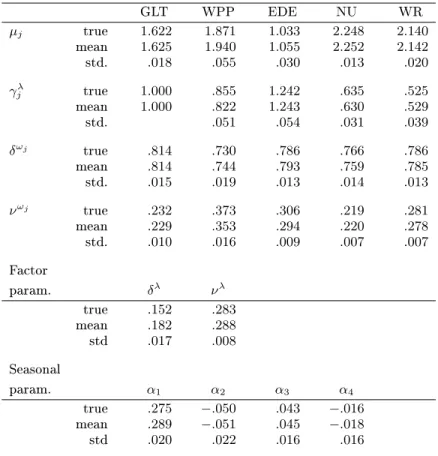
Table 5. ML-EIS for the Poisson Factor Model with Firm Specic Factors and a Common Factor for Simulated Data.
GLT WPP EDE NU WR µj true 1.622 1.871 1.033 2.248 2.140 mean 1.625 1.940 1.055 2.252 2.142 std. .018 .055 .030 .013 .020 γλ j true 1.000 .855 1.242 .635 .525 mean 1.000 .822 1.243 .630 .529 std. .051 .054 .031 .039 δωj true .814 .730 .786 .766 .786 mean .814 .744 .793 .759 .785 std. .015 .019 .013 .014 .013 νωj true .232 .373 .306 .219 .281 mean .229 .353 .294 .220 .278 std. .010 .016 .009 .007 .007 Factor param. δλ νλ true .152 .283 mean .182 .288 std .017 .008 Seasonal param. α1 α2 α3 α4 true .275 −.050 .043 −.016 mean .289 −.051 .045 −.018 std .020 .022 .016 .016
NOTE: The reported numbers are the MC mean and standard deviation of 20 repeated ML-EIS estimates for the parameters for dierent simulated data set and a xed set of CRNs for EIS estimation. ML-EIS estimates are based on a MC sample size ofN= 50and three EIS iterations.
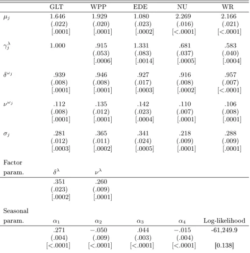
Table 6. ML-EIS for the Negbin Factor Model with Firm Specic Factors and a Common Factor for the TAQ Data.
GLT WPP EDE NU WR µj 1.646 1.929 1.080 2.269 2.166 (.022) (.020) (.023) (.016) (.021) [.0001] [.0001] [.0002] [<.0001] [<.0001] γλ j 1.000 .915 1.331 .681 .583 (.053) (.083) (.037) (.040) [.0006] [.0014] [.0005] [.0004] δωj .939 .946 .927 .916 .957 (.008) (.008) (.017) (.008) (.007) [.0001] [.0001] [.0003] [.0002] [<.0001] νωj .112 .135 .142 .110 .106 (.008) (.012) (.023) (.007) (.008) [.0001] [.0001] [.0004] [.0001] [.0001] σj .281 .365 .341 .218 .288 (.012) (.011) (.024) (.009) (.009) [.0003] [.0002] [.0005] [.0001] [.0001] Factor param. δλ νλ .351 .260 (.023) (.009) [.0002] [.0001] Seasonal param. α1 α2 α3 α4 Log-likelihood .271 −.050 .044 −.015 -61,249.9 (.004) (.009) (.003) (.004) [<.0001] [<.0001] [<.0001] [<.0001] [0.138]
NOTE: The reported numbers are the ML-EIS estimates for the parameters, asymptotic standard errors obtained from a numerical approximation to the Hessian are in parentheses and MC (numerical) standard deviations obtained from 20 ML-EIS estimations conducted under dierent sets of CRNs are in brackets. ML-EIS estimates are based on a MC sample size ofN= 50and three EIS iterations.
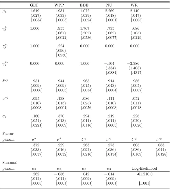
Table 7. ML-EIS for the Negbin Factor Model with Firm- and Industry Specic Factors and a Common Factor for the TAQ Data.
GLT WPP EDE NU WR µj 1.619 1.931 1.072 2.269 2.140 (.027) (.033) (.039) (.018) (.047) [.0034] [.0003] [.0024] [.0001] [.0005] γλ j 1.000 .955 1.767 .735 .686 (.067) (.202) (.062) (.105) [.0022] [.0536] [.0077] [.0229] γτ1 j 1.000 .224 0.000 0.000 0.000 (.096) [.0230] γτ2 j 0.000 0.000 1.000 −.504 −2.386 (.334) (1.408) [.0884] [.4317] δωj .951 .944 .965 .914 .986 (.009) (.009) (.015) (.043) (.005) [.0006] [.0003] [.0034] [.0004] [.0007] νωj .095 .138 .086 .111 .052 (.010) (.013) (.025) (.010) (.011) [.0008] [.0004] [.0056] [.0003] [.0018] σj .160 .370 .294 .219 .226 (.054) (.013) (.041) (.011) (.020) [.0221] [.0009] [.0116] [.0005] [.0026] Factor param. δλ νλ δτ1 ντ1 δτ2 ντ2 .372 .229 .263 .273 .608 .083 (.033) (.016) (.092) (.036) (.086) (.044) [.0037] [.0032] [.0216] [.0134] [.0169] [.0128] Seasonal param. α1 α2 α3 α4 Log-likelihood .262 −.056 .042 −.014 -61,210.0 (.012) (.011) (.009) (.009) [.0005] [.0001] [.0001] [.0001] [1.001]
NOTE: The reported numbers are the ML-EIS estimates for the parameters, asymptotic standard errors obtained from a numerical approximation to the Hessian are in parentheses and MC (numerical) standard deviations obtained from 20 ML-EIS estimations conducted under dierent sets of CRNs are in brackets. ML-EIS estimates are based on a MC sample size ofN= 50and three EIS iterations.
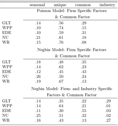
Table 8. Relative Contributions of the Factors to the Overall Variance of the Log Conditional Mean.
seasonal unique common industry
Poisson Model: Firm Specic Factors & Common Factor
GLT .14 .56 .29
WPP .10 .74 .15
EDE .10 .59 .31
NU .21 .61 .18
WR .15 .76 .08
Negbin Model: Firm Specic Factors & Common Factor
GLT .18 .48 .35
WPP .14 .62 .23
EDE .12 .45 .43
NU .26 .50 .24
WR .19 .67 .13
Negbin Model: Firm- and Industry Specic Factors & Common Factor
GLT .14 .35 .22 .29
WPP .14 .64 .21 .01
EDE .11 .30 .55 .03
NU .25 .51 .22 .02
Table 9. Diagnostics Based on the Pearson Residuals.
GLT WPP EDE NU WR
Poisson Model: Firm Specic Factors & Common Factor
Mean .05 .07 .05 .04 .04 Standard dev. 1.24 1.29 1.21 1.20 1.22 Q10 25.0 60.9 6.9 29.6 48.1 (.005) (.000) (.732) (.001) (.000) Q20 56.0 128.1 29.3 62.1 95.4 (.000) (.000) (.080) (.000) (.000)
Negbin Model: Firm Specic Factors & Common Factor
Mean .01 .00 .00 .00 .01 Standard dev. 1.05 1.01 1.01 1.03 1.02 Q10 12.9 27.5 10.6 12.8 31.8 (.228) (.002) (.391) (.237) (.000) Q20 21.2 48.2 21.8 29.3 38.1 (.383) (.000) (.353) (.081) (.008)
Negbin Model: Firm- and Industry Specic Factors & Common Factor
Mean .03 .01 .02 .02 .02 Standard dev. 1.14 1.06 1.09 1.07 1.09 Q10 10.1 20.0 14.8 11.9 15.5 (.428) (.029) (.140) (.229) (.116) Q20 27.1 37.5 28.2 31.5 20.0 (.133) (.010) (.104) (.049) (.454)
Figure 1. Estimated diurnal seasonal eects for the number of trades obtained under the dynamic Poisson factor model with one common factor given byexp{0.275 cos(2πt/75)−0.050 sin(2πt/75)
Figure 2. Truelnθt1 (dashed line) and its smoothed estimates (solid line) for the rst 500 time periods
Figure 3. Time series of the number of trades in 5-minute intervalsytj (top row) and of the standardized