Article No. ectj??????
Time Series Modeling with Duration Dependent
Markov-Switching Vector Autoregressions:
MCMC Inference, Software and Applications
Matteo M. Pelagatti1
Department of Statistics, Universit`a degli Studi di Milano–Bicocca E-mail:[email protected]
Received: February, 2004
Summary Duration dependent Markov-switching VAR (DDMS-VAR) models are time series models with data generating process consisting in a mixture of two VAR processes, which switches according to a two-state Markov chain with transition prob-abilities depending on how long the process has been in a state. In the present paper I propose a MCMC-based methodology to carry out inference on the model’s parameters and introduce DDMSVAR for Ox, a software written by the author for the analysis of time series by means of DDMS-VAR models. An application of the methodology to the U.S. business cycle concludes the article.
Keywords: Markov-switching, business cycle, Gibbs sampling, duration dependence, vector autoregression
1. INTRODUCTION AND MOTIVATION
Since the path-opening paper of Hamilton (1989), many applications of the Markov switching autoregressive model (MS-AR) to the analysis of business cycle have demon-strated its usefulness particularly in dating the cycle in an “objective” way. The basic MS-AR model has, nevertheless, some limitations: (i) it is univariate, (ii) the probability of transition from one state to the other (or to the other ones) is constant. Since busi-ness cycles are fluctuations of the aggregate economic activity, which express themselves through the comovements of many macroeconomic variables, point (i) is not a negligible weakness. The multivariate generalization of the MS model was carried out by Krolzig (1997), in his excellent work on the MS-VAR model. As far as point (ii) is concerned, it is reasonable to believe that the probability of exiting a contraction is not the same at the very beginning of this phase as after several months. Some authors, such as Diebold and Rudebusch (1990), Diebold et al. (1993) and Watson (1994) have found evidence of duration dependence in the U.S. business cycles, and therefore, as Diebold et al. (1993) point out, the standard MS model results miss-specified. In order to face the latter limita-tion, Durland and McCurdy (1994) introduced the duration-dependent Markov switching autoregression, designing an alternative filter for the unobservable state variable. In the present article the duration-dependent switching model is generalized in a multivariate manner, and it is shown how the standard tools of MS-AR model, such as Hamilton’s 1An earlier version of this paper was presented at the 1stOxMetrics User Conference, London 2003.
I would like to thank Prof. David Hendry for useful comments and his encouragement. This work was partially supported by a grant of the Italian Ministry of Education, University and Research (MIUR).
c
°Royal Economic Society 2004. Published by Blackwell Publishers Ltd, 108 Cowley Road, Oxford OX4 1JF, UK and 350 Main Street, Malden, MA, 02148, USA.
filter and Kim’s smoother can be used to model also duration dependence. While Dur-land and McCurdy (1994) carry out their inference on the model by exploiting maximum likelihood estimation, here a multi-move Gibbs sampler is implemented to allow Bayesian (but also finite sample likelihood) inference. The advantages of this technique are that (a) it does not relay on asymptotics1, and in latent variable models, where the unknowns are many, asymptopia can be very far to reach, (b) inference on the latent variables is not conditional on the estimated parameters, but incorporates also the uncertainty on the parameters’ values.
The work is organized as follows: the duration-dependent Markov switching VAR model (DDMS-VAR) is defined in section 2, while the MCMC-based inference is explained in section 3; section 4 briefly illustrates the features of DDMSVAR for Ox, and an applica-tion of the model and of the software to the U.S. business cycle is carried out in secapplica-tion 5.
2. THE MODEL The duration-dependent MS-VAR model2is defined by
yt=µ0+µ1St+A1(yt−1−µ0−µ1St−1) +. . .
+Ap(yt−p−µ0−µ1St−p) +εt (2.1) where yt is a vector of observable variables, St is a binary (0-1) unobservable random variable following a Markov chain with varying transition probabilities,A1, . . . ,Ap are coefficient matrices of a stable VAR process, andεt is a gaussian (vector) white noise with covariance matrixΣ.
In order to achieve duration dependence forSt, the pair (St, Dt) is considered, where Dtis the duration variable defined by
Dt= 1 ifSt6=St−1 Dt−1+ 1 ifSt=St−1 andDt−1< τ Dt−1 ifSt=St−1 andDt−1=τ . (2.2)
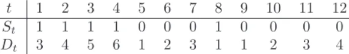
It easy to see that (St, Dt) is also a Markov chain, since conditioning on (St−1, Dt−1) makes (St, Dt) independent of (St−k, Dt−k) with k = 2,3, . . . An example of a possible sample path of (St, Dt) is shown in table 1. The valueτis the maximum that the duration
t 1 2 3 4 5 6 7 8 9 10 11 12
St 1 1 1 1 0 0 0 1 0 0 0 0
Dt 3 4 5 6 1 2 3 1 1 2 3 4
Table 1.A possible realization of the process (St, Dt).
variableDtcan reach and must be fixed so that the Markov chain (St, Dt) is defined on 1Actually MCMC techniques do relay on asymptotic results, but the size of the sample is under control of the researcher and some diagnostics on convergence are available, although this is a field still under development. Here it is meant that the reliability of the inference does not depend on the sample size of the real-world data.
2Using Krolzig’s terminology, we are defining a duration dependent MSM(2)-VAR, that is, Markov-Switching in Mean VAR with two states.
the finite state space
{(0,1),(1,1),(0,2),(1,2), . . . ,(0, τ),(1, τ)}, with finite dimensional transition matrix3
P= 0 p0|1(1) 0 p0|1(2) 0 p0|1(3) . . . 0 p0|1(τ) p1|0(1) 0 p1|0(2) 0 p1|0(3) 0 . . . p1|0(τ) 0 p0|0(1) 0 0 0 0 0 . . . 0 0 0 p1|1(1) 0 0 0 0 . . . 0 0 0 0 p0|0(2) 0 0 0 . . . 0 0 0 0 0 p1|1(2) 0 0 . . . 0 0 .. . ... ... ... ... ... . .. ... ... 0 0 0 0 0 0 . . . p0|0(τ) 0 0 0 0 0 0 0 . . . 0 p1|1(τ) wherepi|j(d) = Pr(St=i|St−1=j, Dt−1=d).
WhenDt=τ, only four events are given non-zero probabilities: (St=i, Dt=τ)|(St−1=i, Dt−1=τ) i= 0,1
(St=i, Dt= 1)|(St−1=j, Dt−1=τ) i6=j, i, j= 0,1 ,
with the interpretation that, when the economy has been in state i at least τ times, the additional periods in which the state remainsiinfluence no more the probability of transition.
As pointed out by Hamilton (1994, section 22.4), it is always possible to write the likelihood function ofyt, depending only on the state variable at timet, even though in the model ap-order autoregression is present; this can be done using the extended state variableS∗
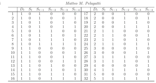
t = (Dt, St, St−1, . . . , St−p), which comprehends all the possible combinations of the states of the economy in the last p periods. In table 2 the state space of non-negligible states4 S∗
t, withp= 4 andτ = 5, is shown. Ifτ ≥pthe maximum number of non-negligible states is given byu=Ppi=12i+ 2(τ−p). The transition matrixP∗of the Markov chainS∗
t is a (u×u) matrix, although rather sparse, having a maximum number 2τ of independent non-zero elements.
In order to reduce the number (2τ) of elements inP∗ to be estimated, a more parsi-monious probit specification is used. Consider the linear model
St•= [β1+β2Dt−1]St−1+ [β3+β4Dt−1](1−St−1) +²t (2.3) with²t∼ N(0,1), and S•
t latent variable defined by Pr(S•
t ≥0|St−1, Dt−1) = Pr(St= 1|St−1, Dt−1) (2.4) Pr(S•
t <0|St−1, Dt−1) = Pr(St= 0|St−1, Dt−1). (2.5)
3The transition matrix is here designed so that the elements of each column, and not of each row, sum to one.
4“Negligible states” stands here for ‘states always associated with zero probability’. For example the state (Dt= 5, St= 1, St−1 = 0, St−2 =s2, St−3 =s3, St−4 =s4), wheres2,s3 ands4 can be either
0 or 1, is negligible as it is not possible forSt to have been 5 periods in the same state, if the state at timet−1 is different from the state at timet.
Dt St St−1 St−2 St−3 St−4 Dt St St−1 St−2 St−3 St−4 1 1 0 1 0 0 0 17 2 0 0 1 0 0 2 1 0 1 0 0 1 18 2 0 0 1 0 1 3 1 0 1 0 1 0 19 2 0 0 1 1 0 4 1 0 1 0 1 1 20 2 0 0 1 1 1 5 1 0 1 1 0 0 21 2 1 1 0 0 0 6 1 0 1 1 0 1 22 2 1 1 0 0 1 7 1 0 1 1 1 0 23 2 1 1 0 1 0 8 1 0 1 1 1 1 24 2 1 1 0 1 1 9 1 1 0 0 0 0 25 3 0 0 0 1 0 10 1 1 0 0 0 1 26 3 0 0 0 1 1 11 1 1 0 0 1 0 27 3 1 1 1 0 0 12 1 1 0 0 1 1 28 3 1 1 1 0 1 13 1 1 0 1 0 0 29 4 0 0 0 0 1 14 1 1 0 1 0 1 30 4 1 1 1 1 0 15 1 1 0 1 1 0 31 5 0 0 0 0 0 16 1 1 0 1 1 1 32 5 1 1 1 1 1
Table 2.State space ofSt∗= (Dt, St, St−1, . . . , St−p) forp= 4, τ= 5.
It’s easy to show that it holds
p1|1(d) = Pr(St= 1|St−1= 1, Dt−1=d) = (2.6) = 1−Φ(−β1−β2d)
p0|0(d) = Pr(St= 0|St−1= 0, Dt−1=d) = Φ(−β3−β4d) (2.7) where d = 1, . . . , τ, and Φ(.) is the standard normal cumulative distribution function. Now four parameters completely define the transition matrixP∗.
3. BAYESIAN INFERENCE ON THE MODEL’S UNKNOWNS In this section it is shown how Bayesian inference on the model’s unknowns
θ= (µ,A,Σ,β,{(St, Dt)}Tt=1), whereµ= (µ0
0,µ01)0 andA= (A1, . . . ,Ap), can be carried out using MCMC methods.
3.1. Priors
In order to exploit conditional conjugacy, the prior joint distribution used is p(µ,A,Σ,β,(S0, D0)) =p(µ)p(A)p(Σ)p(β)p(S0, D0), p(
.
) denoting the generic density or probability function, whereµ∼ N(m0,M0), (3.8) vec(A)∼ N(a0,A0), (3.9) p(Σ)∝ |Σ|−1 2(rank(Σ)+1), (3.10) β∼ N(b0,B0), (3.11) (3.12) andp(S0, D0) is a probability function that assigns a prior probability to every element of the state-space of (S0, D0). Alternatively it is possible to letp(S0, D0) be the ergodic probability function of the Markov chain{(St, Dt)}.
3.2. Gibbs sampling in short
Let θi, i = 1, . . . , I, be a partition of the set θ containing all the unknowns of the model, andθ−i represent the setθ without the elements in θi. In order to implement a Gibbs sampler to sample from the joint posterior distribution of all the unknowns of the model, it is sufficient to find the full conditional posterior distributionp(θi|θ−i,Y), with
Y = (y1, . . . ,yT) and i= 1, . . . , I. A Gibbs sampler step is the generation of a random variate fromp(θi|θ−i,Y),i= 1, . . . , I, where the elements ofθ−iare substituted with the newest values previously generated. Since, under mild regularity conditions, the Markov chain defined for θ(i), where θ(i) is the value of θ generated at the ith iteration of the Gibbs sampler, converges to its stationary distribution, and this stationary distribution is the “true” posterior distributionp(θ|Y), it is sufficient to fix an initial burn-in period of M iterations, such that the Markov chain virtually “forgets” the arbitrary starting values
θ(0), to sample form (an approximation of) the joint posterior distribution. The values obtained for each element of θ are samples from the marginal posterior distribution of each parameters.
3.3. Gibbs sampling steps Step 1. Generation of {S∗
t}Tt=1 It is used an implementation of the multi-move Gibbs sampler originally proposed by Carter and Kohn (1994), which, suppressing the condi-tioning on the other parameters from the notation, exploits the identity
p(S∗ 1, . . . , S∗T|YT) =p(ST∗|YT) TY−1 t=1 p(S∗ t|St+1∗ ,Yt), (3.13) withYt= (y1, . . . ,yt).
Let ˆξt|r be the vector containing the probabilities ofSt∗ being in each state (the first element is the probability of being in state 1, the second element is the probability of being in state 2, and so on) givenYr and the model’s parameters. Letηt be the vector containing the likelihood of each state givenYtand the model’s parameters, whose generic element is (2π)−n/2|Σ|−1/2exp ½ −1 2(yt−yˆt) 0Σ−1(y t−yˆt) ¾ , where ˆ yt=µ0+µ1St+A1(yt−1−µ0−µ1St−1) +. . .+Ap(yt−p−µ0−µ1St−p) changes value according to the state ofS∗
t.
The filtered probabilities of the states can be calculated using Hamilton’s filter ˆ ξt|t= ˆ ξt|t−1¯ηt ˆ ξ0 t|t−1ηt ˆ ξt+1|t=P∗ξˆt|t
with the symbol¯indicating element by element multiplication. The filter is completed with the prior probabilities vector ˆξ1|0, that, as already noticed, can be set equal to the vector of ergodic probabilities of the Markov chain{S∗
To sample from the distribution of{S∗
t}T1 given the full information setYT, it can be used the result
Pr(S∗ t =j|S∗t+1=i,Yt) = Pr(S∗ t+1=i|St∗=j) Pr(St∗=j|Yt) Pm j=1Pr(St+1∗ =i|St∗=j) Pr(St∗=j|Yt) = pi|j ˆ ξ(j)t|t Pm j=1pi|jξˆ(j)t|t ,
wherepi|j is the transition probability of moving to stateifrom statej(element (i, j) of the transition matrixP∗) andξ(j)
t|t is thej-th element of vectorξt|t. In matrix notation the same can be written as
ˆ ξt|(S∗ t+1=i,YT)= pi.¯ξˆt|t p0i.ξˆ t|t (3.14) wherep0i. denotes thei-th row of the transition matrixP∗.
Now all the probability functions in equation (3.13) have been given a form, and the states can, thus, be generated starting from the filtered probability ˆξT|T and proceeding backward (T−1, . . . ,1), using equation (3.14) where iis to be substituted with the last generated values∗
t+1.
Once a set of sampled {S∗
t}Tt=1 has been generated, it is automatically available a sample for{St}T
t=1 and{Dt}Tt=1.
The advantage of using the described multi-move Gibbs sampler, compared to the sin-gle move Gibbs sampler that can be implemented as in Carlin et al. (1992), or using the software BUGS, is that the whole vector of states is sampled at once, improving signifi-cantly the speed of convergence of the Gibbs samper’s chain to its ergodic distribution. Kim and Nelson (1999, section 10.3), in their outstanding monograph on state-space models with regime switching, use a single-move Gibbs sampler (12000 sample points) to achieve (almost) the same goal as in this paper, but my experience with the slow con-vergence properties of the single-move sampler does not convince me on the reliability of their estimates.
Step 2. Generation of (A,Σ) Conditionally on {St}T
t=1 and µ equation (2.1) is just a multivariate normal (auto-)regression model for the variable y∗
t = yt−µ0−µ1St, whose parameters, given the discussed prior distribution, have the following posterior distributions, known in literature. LetX be the matrix, whosetth column is
x
.t
= y∗ t y∗ t−1 .. . y∗ t−p ,fort= 1, . . . , T, and letY∗= (y∗
1, . . . ,yT∗).
The posterior for (vec(A),Σ) is, suppressing the conditioning on the other parameters, the normal–inverse Wishart distribution
p(vec(A),Σ|Y,X) =p(vec(A)|Σ,Y,X)p(Σ|Y,X) p(Σ|Y,X) density of aIWk(V, n−m)
with
V =Y∗Y∗0−Y∗X0(XX0)−1XY∗0 A1= (A−01+XX0Σ−1)−1
a1=A1[A−01a0+ (X⊗Σ−1)vec(Y)].
Step 3. Generation ofµ Conditionally onAandΣ, by multiplying both sides of equa-tion (2) times
A(L) = (I−A1L−. . .−ApLp), where L is the lag operator, we obtain
A(L)yt=µ0A(1) +µ1A(L)St+εt,
which is a multivariate normal linear regression model with known varianceΣ, and can be treated as shown in step 2., with respect to the specified prior forµ.
Step 4. Generation ofβ Conditionally on{S∗
t}Tt=1, consider the probit model described in section 2. Albert and Chib (1993) have proposed a method based on a data augmenta-tion algorithm to draw from the posterior of the parameters of a probit model. Given the parameter vectorβ of last iteration of the Gibbs sampler, generate the latent variables
{S•
t} from the respective truncated normal densities S• t|(St= 0,xt,β)∼ N(x0tβ,1)I(−∞,0) S• t|(St= 1,xt,β)∼ N(x0tβ,1)I[0,∞) with β= (β1, β2, β3, β4)0 xt= (St−1, Dt−1,(1−St−1),(1−St−1)Dt−1)0 (3.15) andI{
.
} indicator function used to denote truncation.With the generatedS•
t’s the probit regression equation (2.3) becomes, again, a normal linear model with known variance.
The former Gibbs samper’s steps were numbered from 1 to 4, but any ordering of the steps would eventually bring to the same ergodic distribution.
4. THE SOFTWARE
DDMSVAR for Ox5 is a software for time series modeling with DDMS-VAR processes that can be used in three different ways: (i) as a menu driven package6, (ii) as an Ox object class, (iii) as a software library for Ox. The DDMSVAR software is freely available7at the author’s internet sitewww.statistica.unimib.it/utenti/p matteo/. In this section I give a brief description of the software and in next section I illustrate its use with a real-world application.
5Ox (Doornik, 2001) is an object-oriented matrix programming language freely available for the aca-demic community in its console version.
6If run with the commercial version of Ox (OxProfessional).
7The software is freely available and usable (at your own risk): the only condition is that the present article should be cited in any work in which the DDMSVAR software is used.
4.1. OxPack version
The easiest way to use DDMSVAR is adding the package8to OxPack giving DDMSVAR as class name. The following steps must be followed to load the data, specify the model and estimate it.
Formulate
Open a database, choose the time series to model and give them theY variablestatus. If you wish to specify an initial series of state variables, this series has to be included in the database and, once selected in the model variables’ list, give it theState variable init
status; otherwise DDMSVAR assigns the state variable’s initial values automatically.
Model settings
Chose the order of the VAR model (p), the maximal duration (tau), which must be at least9 2, and write a comma separated list of percentiles of the marginal posterior distributions, that you want to read in the output (default is2.5,50,97.5).
Estimate/Options
At the moment only the illustrated Gibbs sampler is implemented, but EM algorithm based maximum-likelihood estimation is in the to-do list for the next versions of the software. So choose the sample of data to model and pressOptions.... The options window is divided in three areas.
iterations
Here you choose the number of iteration of the Gibbs sampler, and the number of burn in iteration, that is, the amounts of start iterations that will not be used for estimation, because too much influenced by the arbitrary starting values. Of course the latter must be smaller than the former.
priors & initial values
If you want to specify prior means and variances of the parameters to estimate, do it in a .in7 or .xls database following these rules: prior means and variances for the vectorization of the autoregressive matrixA= [A1,A2, . . . ,Ap] must be in fields with namesmean a andvar a; prior means and variances for the mean vectorsµ0 andµ1 must be in fields with namesmean mu0, var mu0, mean mu1andvar mu1; the fields for the vectorβ are to be namedmean beta andvar beta. The file name is to be specified with extension. If you don’t specify the file, DDMSVAR uses priors that are vague for typical applications. The file containing the initial values for the Gibbs sampler needs also to be a database in .in7 or .xls format, with fieldsafor vec(A),mu0forµ0,mu1forµ1,sigmafor vech(Σ) andbetaforβ. If no file is specified, DDMSVAR assigns initial values automatically. saving options
In order to save the Gibbs sample generated by DDMSVAR, specify a file name (you 8At the moment the DDMSVAR03.oxo file.
9If you wish to estimate a classical MS-VAR model, choosetau = 2and use priors for the parameters
β2 andβ4 that put an enormous mass of probability around 0. This will prevent the duration variable
from having influence in the probit regression. The maximal usable value fortau depends only on the power of your computer, but have care that the dimensions of the transition matrixu×udon’t grow too much, or the waiting time may become unbearable.
don’t need to write the extension, at the moment the only format available is .in7) and checkSave also state seriesif the specified file should contain also the samples of the state variables. CheckProbabilities of state 0 infilename.extto save the smoothed probabilities
{Pr(St= 0|YT)}Tt=1 in the database from which the time series are taken.
Program’s Output
Since Gibbs sampling may take a long time, after five iterations the program prints an estimate of the waiting time. The user is informed of the progress of the process every 100 iterations.
At the end of the iteration process, the estimated means, standard deviations (in the output named standard errors), percentiles of the marginal posterior distributions are given.
The output consists also in a number of graphs: 1 probabilities ofSt being in state 0 and 1,
2 mean and percentiles of the transition probabilities distributions with respect to the duration,
3 autocorrelation function of every sampled parameter (the faster it dies out, the higher the speed of the Gibbs sampler in exploring the posterior distribution’s sup-port, and the smaller the number of iteration needed to achieve the same estimate’s precision),
4 kernel density estimates of the marginal posterior distributions,
5 Gibbs sample graphs (to check if the burn in period is long enough to ensure that the initial values have been “forgot”),
6 running means, to visually check the convergence of the Gibbs sample means.
4.2. The DDMSVAR() object class
The second simplest way to use the software is creating an instance of the object DDMSVAR and using its member functions. The best way to illustrate the most relevant member functions of the class DDMSVAR is showing a sample program and commenting it.
#include "DDMSVAR.ox" main() {
decl dd = new DDMSVAR(); dd->LoadIn7("USA4.in7");
dd->Select(Y_VAR, {"DLIP", 0, 0, "DLEMP", 0, 0,
"DLTRADE", 0, 0, "DLINCOME",0 ,0}); dd->Select(S_VAR,{"NBER", 0, 0}); dd->SetSelSample(1960, 1, 2001, 8); dd->SetVAROrder(0); dd->SetMaxDuration(60); dd->SetIteration(21000); dd->SetBurnIn(1000); dd->SetPosteriorPercentiles(<0.05,50,99.5>);
dd->SetPriorFileName("prior.in7"); dd->SetInitFileName("init.in7"); dd->SetSampleFileName("prova.in7",TRUE); dd->Estimate(); dd->StatesGraph("states.eps"); dd->DurationGraph("duration.eps"); dd->Correlograms("acf.eps", 100); dd->Densities("density.eps"); dd->SampleGraphs("sample.eps"); dd->RunningMeans("means.eps"); }
ddis declared as instance of the object DDMSVAR. The first four member functions are an inheritance of the class Database and will not be commented here10. Notice only that the variable selected in theS VARgroup must contain the initial values for the state variable time series. Nevertheless, if no series is selected asS VAR, DDMSVAR calculates initial values for the state variables automatically.
SetVAROrder(const iP)sets the order of the VAR model to the integer valueiP. SetMaxDuration(const iTau)sets the maximal duration to the integer valueiTau. SetIteration(const iIter)sets the number of Gibbs sampling iterations to the inte-ger valueiIter.
SetBurnIn(const iBurn) sets the number of burn in iterations to the integer value iBurn.
SetPosteriorPercentiles(const vPerc) sets the percentiles of the posterior distri-butions that have to be printed in the output. vPerc is a row vector containing the percentiles (in %).
SetPriorFileName(const sFileName),
SetInitFileName(const sFileName)are optional; they are used to specify respectively the file containing the prior means and variances of the parameters and the file with the initial values for the Gibbs sampler (see the previous subsection for the format that the two files need to have). If they are not used, priors are vague and initial values are automatically calculated.
SetSampleFileName(const sFileName, const bSaveS)is optional; if used it sets the file name for saving the Gibbs sample and if bSaveSisFALSEthe state variables are not saved, otherwise they are saved in the same file sFileName. sFileNamedoes not need the extension, since the only available format is .in7.
Estimate() carries out the iteration process and generates the textual output (if run within GiveWin-OxRun it does also the graphs). After 5 iteration the user is informed of the expected waiting time and every 100 iterations also about the progress of the Gibbs sampler.
StatesGraph(const sFileName), DurationGraph(const sFileName),
Correlograms(const sFileName, const iMaxLag), Densities(const sFileName),
SampleGraphs(const sFileName),
RunningMeans(const sFileName)are optional and used to save the graphs described in the last subsection.sFileNameis a string containing the file name with extension (.emf, .wmf, .gwg, .eps, .ps) and iMaxLag is the maximum lag for which the autocorrelation funtcion should be calculated.
4.3. DDMSVAR software library
The last and most complicated (but also flexible) way to use the software is as library of functions. The DDMS-VAR library consists in 25 functions, but the user need to know only the following 10. Throughout the function list, it is used the notation below. p scalar order of vector autoregression (VAR(p))
tau scalar maximal duration (τ)
k scalar number of time series in the model
T scalar number of observations of thek time series u scalar dimension of the state space of{S∗
t} (u=Ppi=12i+ 2(τ−p))
Y (k×T) matrix of observation vectors (YT) s (T×1) vector of current state variable (St) mu0 (k×1) vector of means when the state is 0 (µ0)
mu1 (k×1) vector of mean-increments when the state is 1 (µ1) A (k×pk) VAR matrices side by side ([A1, . . . ,Ap])
Sig (k×k) covariance matrix of VAR error (Σ)
SS (u×p+2) state space of the complete Markov chain{S∗}(tab. 2) pd (tau×4) matrix of the probabilities [p00(d), p01(d), p10(d), p11(d)] P (u×u) transition matrix relative to SS (P∗)
xi flt (u×T−p) filtered probabilities ([ ˆξt|t]) eta (u×T−p) matrix of likelihoods ([ηt])
ddss(p,tau)
Returns the state space SS (see table 2). A sampler(Y,s,mu0,mu1,p,a0,pA0)
Carry out step 2. of the Gibbs sampler, returning a sample point from the posterior of vec(A) witha0andpA0being respectively the prior mean vector and the prior precision matrix (inverse of covariance matrix) of vec(A).
mu sampler(Y,s,p,A,Sig,m0,pM0)
Carry out step 3. of the Gibbs sampler, returning a sample point from the posterior of [µ0
0,µ01]0withm0andpM0being respectively the prior mean vector and the prior precision matrix (inverse of covariance matrix) of [µ0
0,µ01]0. probitdur(beta,tau)
Returns the matrix pd containing the transition probabilities for every duration d = 1,2, . . . , τ. pd = p0|0(1) p0|1(1) p1|0(1) p1|1(1) p0|0(2) p0|1(2) p1|0(2) p1|1(2) .. . ... ... ... p0|0(τ) p0|1(τ) p1|0(τ) p1|1(τ) . ddtm(SS,pd)
Puts the transition probabilitiespdinto the transition matrix relative to the chain with state spaceSS.
ergodic(P)
Returns the vectorxi0of ergodic probabilities of the chain with transition matrixP. msvarlik(Y,mu0,mu1,Sig,A,SS)
Returnseta, matrix ofT columns of likelihood contributions for every possible state in SS.
ham flt(xi0,P,eta)
Returns xi flt, matrix of T columns of filtered probabilities of being in each state in SS.
state sampler(xi flt,P)
Carry out step 1. of the Gibbs sampler. It returns a sample time series of values drawn from the chain with state spaceSS, transition matrixPand filtered probabilitiesxi flt. new beta(s,X,lastbeta,diffuse,b,B0)
Carry out step 4. of the Gibbs sampler. It returns a new sample point from the posterior of the vectorβ, given the dependent variables in X, where the generic row is given by (3.15). If diffuse6= 0, a diffuse prior is used.
5. DURATION DEPENDENCE IN THE U.S. BUSINESS CYCLE
The model and the software illustrated in the previous sections have been applied to 100 times the difference of the logarithm of the four time series, on which the NBER relays to date the U.S. business cycle, dating from January 1960 to August 2001: i) industrial production (IP), ii) total nonfarm-employment (EMP), iii) total manufacturing and trade sales in million of 1996$ (TRADE), iv) personal income less transfer payments in billions of 1996$ (INCOME).
The model, with p = 2 did not work too well, while the results in absence of the VAR part (p= 0) and maximal durationτ= 120 (10yrs) are rather encouraging: this is
Figure 1.(Smoothed) probability of recession (line) and NBER dating (gray shade) 1960 1965 1970 1975 1980 1985 1990 1995 2000 0.1 0.2 0.3 0.4 0.5 0.6 0.7 0.8 0.9 1.0
probably due to the fact that the duration dependent MS model is a stationary process, which, therefore, can be arbitrarily well approximated by an autoregressive process. As a result the duration dependent switching part and the VAR part of the model try to “explain” almost the same features (autocorrelation) of the series, and the model is not too well identified.
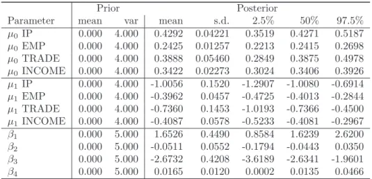
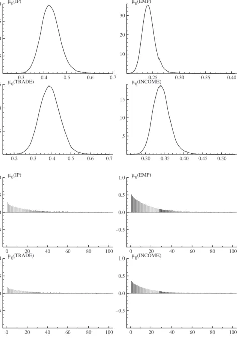
The inference on the model unknowns is based on a Gibbs sample of 21000 points, the first 1000 of which were discarded. In appendix the correlograms and the kernel density estimates for each parameter are reported. All the correlograms die out before the 100th lag, thus the choice of a burn-in sample of 1000 points seems quite reasonable11.
An earlier experiment withτ= 60 (5yrs) was carried out, but it is not reported here: the results were quite similar to the ones reported below and the conclusions the same.
Summaries of the marginal posterior distributions are shown in table 3, while figure 1 compares the probability of the U.S. economy being in recession resulting from the estimated model with the official NBER dating: the signal “probability of being in re-cession” extracted by the model here presented matches the official dating rather well, and is less noisy than the signal extracted by Hamilton (1989), based on the IP series only. The NBER dating seems to be best matched if, every time the model’s probability of being in recession exceeds 0.5, the peak date is set equal the time the line crosses a low probability level (say 0.1) from below and the trough date is set equal the time the probability line crosses a high probability level (say 0.9) from above. NBER trough dates seem to be matched more frequently by the model than the peaks.
Figure 2 shows how the duration of a state (recession or expansion) influences the tran-sition probabilities: while the probability of moving from a recession into an expansion seems to be influenced by the duration of the recession, the probability of falling into a recession appears to be independent of the length of the expansion.
Table 3.Description of the prior and posterior distributions of the model’s parameters.
Prior Posterior
Parameter mean var mean s.d. 2.5% 50% 97.5% µ0 IP 0.000 4.000 0.4292 0.04221 0.3519 0.4271 0.5187 µ0 EMP 0.000 4.000 0.2425 0.01257 0.2213 0.2415 0.2698 µ0 TRADE 0.000 4.000 0.3888 0.05460 0.2849 0.3875 0.4978 µ0 INCOME 0.000 4.000 0.3422 0.02273 0.3024 0.3406 0.3926 µ1 IP 0.000 4.000 -1.0056 0.1520 -1.2907 -1.0080 -0.6914 µ1 EMP 0.000 4.000 -0.3962 0.0457 -0.4725 -0.4013 -0.2844 µ1 TRADE 0.000 4.000 -0.7360 0.1453 -1.0193 -0.7366 -0.4500 µ1 INCOME 0.000 4.000 -0.4087 0.0578 -0.5233 -0.4081 -0.2967 β1 0.000 5.000 1.6526 0.4490 0.8584 1.6239 2.6200 β2 0.000 5.000 -0.0511 0.0552 -0.1794 -0.0443 0.0350 β3 0.000 5.000 -2.6732 0.4208 -3.6189 -2.6341 -1.9601 β4 0.000 5.000 0.0165 0.0120 0.0002 0.0135 0.0466 6. CONCLUSIONS
The model proved to have a good capability of discerning recessions and expansions, as the probabilities of recession tend to assume very low or very high values and, the resulting dating of the U.S. business cycle is very close to the official one.
As far as duration-dependence is concerned, my results are similar to those of Diebold and Rudebusch (1990), Diebold et al. (1993), Sichel (1991) and Durland and McCurdy (1994): U.S. recessions are duration dependent, while expansions seem to be not duration dependent. This could be simply due to the fact that governments are interested in exiting
Figure 2.Mean (solid), median (dash) and 95% credible interval (dots) of the posterior
distribution of the probability of moving a) from a recession into an expansion after d months of recession b) from an expansion to a recession afterdmonths of expansion
0 10 20 30 40 50 60 70 80 90 100 110 120 0.25 0.50 0.75 1.00 a) 0 10 20 30 40 50 60 70 80 90 100 110 120 0.25 0.50 0.75 1.00 b) c
contractions, while the opposite is not true, and the policies they put in practice in order to achieve this goal seem effective.
The DDMSVAR software has demonstrated to work fine, even though I must recognize that it is far from being fully optimized: there is too much looping in the code for an interpreted, although very efficient, language as Ox. Future versions will be more efficient. The Gibbs sampling approach has many advantages but also a big disadvantage: the former are that (i) it allows prior information to be exploited, (ii) it avoids the computa-tional problems pointed out by Hamilton (1994) that can arise with maximum likelihood estimation, (iii) it does not relay on asymptotic inference (read note 1.), (iv) the infer-ence on the state variables is not conditional on the set of estimated parameters. The big disadvantage is a long computation time: the 21000 Gibbs sampler iterations generated for last section’s results took more than 13 hours12.
REFERENCES
Albert, J. H. and S. Chib (1993). Bayesian analysis of binary and polychotomous responce data. Journal of the American Statistical Association 88, 669–79.
Carlin, B. P., N. G. Polson, and D. S. Stoffer (1992). A Monte Carlo approach to nonnormal and nonlinear state-space modeling. Journal of the American Statistical Association 87, 493–500.
Carter, C. K. and R. Kohn (1994). On Gibbs sampling for state space models.
Biometrika 81, 541–53.
Diebold, F. and G. Rudebusch (1990). A nonparametric investigation of duration depen-dence in the American business cycle. Journal of Political Economy 98, 596–616. Diebold, F., G. Rudebusch, and D. Sichel (1993). Further evidence on business cycle
duration dependence. In J. Stock and M. Watson (Eds.), Business Cycles, Indicators and Forcasting. The University of Chicago Press.
Doornik, J. A. (2001).Ox. An object-oriented matrix programming language. Timberlake Consultants Ltd.
Durland, J. and T. McCurdy (1994). Duration–dependent transitions in a Markov model of U.S. GNP growth. Journal of Business and Economic Statistics 12, 279–288. Hamilton, J. D. (1989). A new approach to the economic analysis of nonstationary time
series and the business cycle. Econometrica 57, 357–384.
Hamilton, J. D. (1994). Time Series Analysis. Princeton University Press.
Kim, C. J. and C. R. Nelson (1999). State-space models with regime switching: classical and Gibbs-sampling approches with applications. The MIT Press.
Krolzig, H.-M. (1997). Markov-Switching Vector Autoregressions. Modelling, Statistical Inference and Application to Business Cycle Analysis. Springer-Verlag.
Sichel, D. E. (1991). Business cycle duration dependence: a parametric approach.Review of Economics and Statistics 73, 254–256.
Watson, J. (1994). Business cycle durations and postwar stabilization of the U.S. econ-omy. American Economic Review 84, 24–46.
APPENDIX
Figure 3.Kernel density estimates and correlograms ofµ0.
0.3 0.4 0.5 0.6 0.7 2.5 5.0 7.5 10.0 µ0(IP) 0.25 0.30 0.35 0.40 10 20 30 µ0(EMP) 0.2 0.3 0.4 0.5 0.6 0.7 2.5 5.0 7.5 µ0(TRADE) 0.30 0.35 0.40 0.45 0.50 5 10 15 µ0(INCOME) 0 20 40 60 80 100 −0.5 0.0 0.5 1.0 µ0(IP) 0 20 40 60 80 100 −0.5 0.0 0.5 1.0 µ0(EMP) 0 20 40 60 80 100 −0.5 0.0 0.5 1.0 µ0(TRADE) 0 20 40 60 80 100 −0.5 0.0 0.5 1.0 µ0(INCOME)
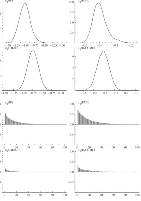
Figure 4.Kernel density estimates and correlograms ofµ1. −1.50 −1.25 −1.00 −0.75 −0.50 −0.25 0.00 1 2 µ1(IP) −0.5 −0.4 −0.3 −0.2 2.5 5.0 7.5 10.0 µ1(EMP) −1.50 −1.25 −1.00 −0.75 −0.50 −0.25 0.00 1 2 µ1(TRADE) −0.6 −0.5 −0.4 −0.3 −0.2 −0.1 2 4 6 µ1(INCOME) 0 20 40 60 80 100 −0.5 0.0 0.5 1.0 µ1(IP) 0 20 40 60 80 100 −0.5 0.0 0.5 1.0 µ1(EMP) 0 20 40 60 80 100 −0.5 0.0 0.5 1.0 µ1(TRADE) 0 20 40 60 80 100 −0.5 0.0 0.5 1.0 µ1(INCOME)
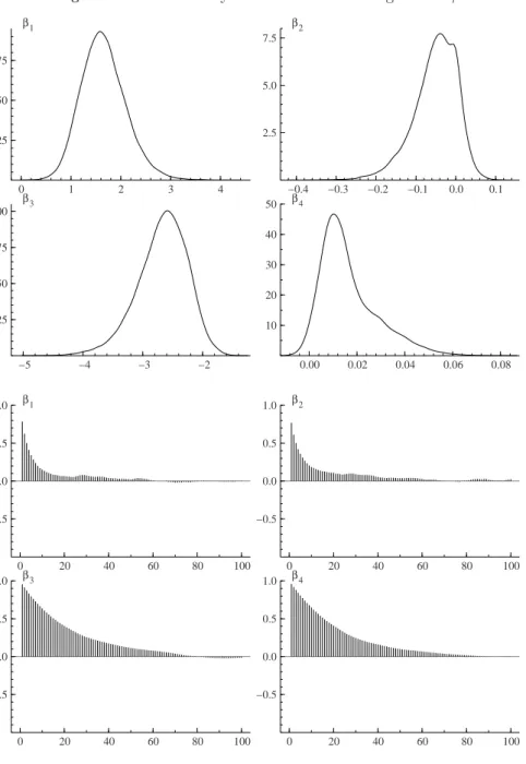
Figure 5.Kernel density estimates and correlograms ofβ. 0 1 2 3 4 0.25 0.50 0.75 β1 −0.4 −0.3 −0.2 −0.1 0.0 0.1 2.5 5.0 7.5 β2 −5 −4 −3 −2 0.25 0.50 0.75 1.00 β3 0.00 0.02 0.04 0.06 0.08 10 20 30 40 50 β4 0 20 40 60 80 100 −0.5 0.0 0.5 1.0 β1 0 20 40 60 80 100 −0.5 0.0 0.5 1.0 β2 0 20 40 60 80 100 −0.5 0.0 0.5 1.0 β3 0 20 40 60 80 100 −0.5 0.0 0.5 1.0 β4
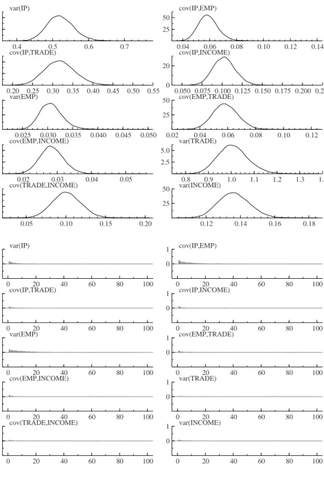
Figure 6.Kernel density estimates and correlograms ofΣ. 0.4 0.5 0.6 0.7 5 10 var(IP) 0.04 0.06 0.08 0.10 0.12 0.14 25 50 cov(IP,EMP) 0.20 0.25 0.30 0.35 0.40 0.45 0.50 0.55 5 10 cov(IP,TRADE) 0.050 0.075 0.100 0.125 0.150 0.175 0.200 0.225 0 20 cov(IP,INCOME) 0.025 0.030 0.035 0.040 0.045 0.050 100 200 var(EMP) 0.02 0.04 0.06 0.08 0.10 0.12 25 50 cov(EMP,TRADE) 0.02 0.03 0.04 0.05 50 100 cov(EMP,INCOME) 0.8 0.9 1.0 1.1 1.2 1.3 1.4 2.5 5.0 var(TRADE) 0.05 0.10 0.15 0.20 10 20 cov(TRADE,INCOME) 0.12 0.14 0.16 0.18 25 50 var(INCOME) 0 20 40 60 80 100 0 1 var(IP) 0 20 40 60 80 100 0 1 cov(IP,EMP) 0 20 40 60 80 100 0 1 cov(IP,TRADE) 0 20 40 60 80 100 0 1 cov(IP,INCOME) 0 20 40 60 80 100 0 1 var(EMP) 0 20 40 60 80 100 0 1 cov(EMP,TRADE) 0 20 40 60 80 100 0 1 cov(EMP,INCOME) 0 20 40 60 80 100 0 1 var(TRADE) 0 20 40 60 80 100 0 1 cov(TRADE,INCOME) 0 20 40 60 80 100 0 1 var(INCOME)