Research Paper
Outlier Detection using Graph Mining
On individuals in the Enron email datasetAuthor:
B.Sc. Tessa van der Eems
Supervisors:
Dr. Evert Haasdijk
Vrije Universiteit Amsterdam
Drs. Scott Mongeau
Deloitte Nederland Nyenrode Business Universiteit
Computational Intelligence Group Department of Computer Science
I have written this research paper as part of the Master’s program Business Analytics at the Vrije Universiteit Amsterdam. The Master’s program consists of three main parts: applied mathematics, computer science and economics. The aim of this research is to perform research using the knowledge gained during the Master’s program on a particular practical problem.
In this paper, we conducted research on the topic of outlier detection using graph min-ing. More precise, using graph visualization, statistics and querymin-ing. I chose this topic because of several reasons. First of all, I gained some experience in fraud analysis at my work at Deloitte, which is part of the Dual Master’s program. Furthermore, I followed multiple courses concerning graphs at both the Vrije Universiteit and Deloitte, and these courses elevated my interest. Finally, the topic is rather new and unexplored, making it an interesting topic for research.
I conducted this research at Deloitte, at the Analytics and Discovery team of the Risk Services service line. This team supports other teams of Risk Services with data analytics but also performs analytics directly for clients. Currently, we are expanding to more advanced analytics, among others, graph databases, machine learning and text mining. Whereas, I focus, together with Scott Mongeau, Manager Analytics at Deloitte, on the techniques of graph mining.
Hereby, I want to thank my supervisors, Dr. Evert Haasdijk of the Vrije Universiteit Am-sterdam and Drs. Scott Mongeau, Analytics Manager at Deloitte Netherlands, for their support and dedication. Furthermore, I would like to thank Patrick van Rietschoten, my boyfriend, for his extended help to get this paper to the way it is now.
Outlier detection is an important method for finding possible fraudulent individuals or transactions in a large dataset. When we convert a dataset to the form of a graph, we can use graph mining to allocate outliers.
Graph mining consists of multiple techniques to analyze the graph. Examples are chang-ing the layout of the graph, the rankchang-ing of the nodes, the partitionchang-ing of the nodes and the filtering on the nodes. Other techniques include link analysis, cluster analysis, clas-sification of edges or characteristics of nodes and anomaly detection on edges and nodes of the graph. Furthermore, we can use graph querying to find particular patterns in the graph which can indicate possible fraudulent activities.
In this paper, we investigate whether it is possible to detect outliers by using the com-ponents of graph mining. For this purpose we have used the Enron email dataset, which contains all emails sent between Enron employees between 1998 and 2002. Note that, we only look at the sender and receivers of the email to create the corresponding network. We created a network based on the senders and receivers in the Enron email dataset, whereas, the weight of the edge between two individuals is the sum of the number of emails between them. First, we use visualization techniques to analyze the graph. Second we use statistics, where we use the generated graph of visualization. With each technique, we try to use information gathered by previously.
Main findings
We used the techniques ranking and partitioning, which are visualization techniques. We found three possible fraudulent individuals (one is debatable) out of five individuals for the ranking technique. For the indication, whether, someone is possible fraudulent we used a web search. Furthermore, the two individuals who had a much higher ranking value than the others, were both indicated as possible fraudulent. However, for the tech-nique partitioning, the three individuals that were selected were not possible fraudulent.
a web search we indicated her as possible fraudulent. Furthermore, we looked at hubs and authorities using statistics, of the nine individuals we found, we indicated four as possible fraudulent. Therefore, we conclude that it is possible to perform outlier detec-tion on a network using graph mining to indicate possible fraudulent individuals in a communication network.
Recommendations
We have found that visualization and statistics work well by themselves. However, when we use the components and their results together the real value of graph mining comes forward. Furthermore, we recommend creating attributes for the nodes because then more techniques can be used to analyze the graph. At last, we recommend starting with the layout of the graph because this technique gives a good first overview of the structure of the data.
Preface i Executive Summary ii Main findings . . . ii Recommendations . . . iii Contents iv List of Figures vi List of Tables vii 1 Introduction 1 1.1 Goal and research question . . . 2
1.2 Research company . . . 2 1.3 Outline . . . 2 2 Techniques 3 2.1 Graph visualization. . . 4 2.1.1 Layout. . . 4 2.1.2 Ranking . . . 7 2.1.3 Partitioning . . . 8 2.1.4 Filtering. . . 9 2.1.5 Further reading . . . 9 2.2 Graph statistics . . . 10 2.2.1 Link analysis . . . 10 2.2.2 Cluster analysis. . . 10 2.2.3 Classification . . . 11 2.2.4 Anomaly detection . . . 11 2.2.5 Further reading . . . 11 2.3 Graph querying . . . 12 2.3.1 Patterns . . . 12 2.3.2 NoSQL Databases . . . 13 2.3.3 Further reading . . . 14 iv
3 Related Research 15
3.1 Research regarding graph mining . . . 15
3.2 Research regarding outlier detection . . . 16
3.3 Research regarding the Enron corpus . . . 16
4 Experimental Data 18 4.1 Case . . . 18 4.2 Description . . . 19 4.3 Preparation . . . 20 4.4 Characteristics . . . 21 5 Experimental Setup 22 5.1 Graph visualization. . . 23 5.2 Graph statistics . . . 24 5.3 Graph querying . . . 25
6 Results and Interpretations 26 6.1 Graph visualization. . . 26
6.2 Graph statistics . . . 31
7 Conclusions and Future Research 34 7.1 Conclusions . . . 34 7.2 Limitations . . . 35 7.3 Future research . . . 36 A Terminology 37 B Tools 40 B.1 Graph visualization. . . 40 B.2 Graph statistics. . . 41 B.3 Graph querying . . . 41 C Mailboxes 43 D Fraudulent References 44 Bibliography 46
2.1 Example of an undirected graph . . . 4
2.2 Example of a graph with circular layout . . . 5
2.3 Example of a graph with concentric layout. . . 5
2.4 Example of a graph with force atlas layout. . . 6
2.5 A complex undirected graph, with ranking applied . . . 7
2.6 A complex undirected graph, with partitioning applied . . . 8
2.7 A complex undirected graph, with filtering applied . . . 9
2.8 Examples of patterns . . . 12
2.9 An example of a graph with relations. . . 13
4.1 Enron’s logo by Paul Rand . . . 18
4.2 Histogram of the number of mails sent and received for each individual in the Enron dataset . . . 21
5.1 Interaction between the graph mining techniques . . . 22
6.1 Results of graph visualization after adjusting the layout . . . 26
6.2 Results of graph visualization after applying filtering on the graph of Figure 6.1 . . . 27
6.3 Results of graph visualization after adjusting the layout on the graph of Figure 6.2 . . . 27
6.4 Results of graph visualization after using ranking on the nodes of the graph in Figure 6.3 . . . 28
6.5 Results of graph visualization after using partitioning on the nodes, with the outliers circled, on the graph of Figure 6.4 . . . 29
6.6 Results of graph visualization after using partitioning on the nodes, with the outliers circled, on the graph of Figure 6.5 . . . 30
A.1 Example of a undirected graph . . . 37
A.2 Example of a directed graph. . . 37
B.1 Examples of graph visualization tools . . . 41
2.1 Legend of Figure 2.5 . . . 7
2.2 Distribution of classes of Figure 2.6. . . 8
5.1 Parameter settings graph visualization setup . . . 23
5.2 Parameter settings graph statistics setup. . . 24
6.1 Individuals with the highest eigenvalue centrality and an indication if they were fraudulent . . . 28
6.2 Outliers of Figure 6.6 and an indication if they were fraudulent . . . 30
6.3 Individuals that both belong to the egocentric network of Louise Kitchen and John Lavorato . . . 31
6.4 Individuals with the strongest connection to both Louise Kitchen and John Lavorato and an indication if they were fraudulent . . . 31
6.5 Individuals with the highest authority score and an indication if they were fraudulent . . . 32
6.6 Individuals with the highest hub score and an indication if they were fraudulent . . . 32
A.1 Degree, In-degree and Out-degree of the graphs in Figures A.1 and A.2 . 39 C.1 Mailboxes present in the Enron dataset . . . 43
D.1 Employees and their functions of Enron (1) . . . 44
D.2 Employees and their functions of Enron(2). . . 45
Introduction
Graph mining is analyzing a dataset, represented as a graph, which consists of nodes (entities) and edges (relationships). It consists of several components; the most promi-nent are visualization, statistics and querying. Each of these techniques can be used by itself, however, the real value of graph mining comes forward when these are combined. The techniques used by Facebook and LinkedIn are, amongst others, famous examples of graph mining. These websites use the network of friendships and connections to sug-gest likely new ones. They use predictive methods based on graphs to calculate the probability of each connection to exist in the future.
Another possible application of graph mining is outlier detection. Outlier detection is identifying transactions, individuals, etc. from a large search space, which differentiate in some way from the total population. Research on outlier detection focuses mostly on fraudulent outliers. Examples of this are credit card fraud and ATM card skimming. Moreover, large banks spend a significant amount of money on online outlier detection. When a transaction differs from the natural pattern of the card and of the overall pattern, the card will be disabled.
In this research paper, we use graph mining to detect outliers in the Enron email dataset. Enron was an American company that went bankrupt in 2001. After a thorough investi-gation, multiple fraudulent activities were discovered. We will only focus on the network, represented by the emails, in the dataset. The content of the emails is, therefore, out of scope for us.
1.1
Goal and research question
In this research paper, we will be investigating in what manner we can use graph mining, consisting of visualization, statistics and querying as a tool for outlier analysis. We look at how these parts perform separately and how they can be combined to achieve an interaction effect between them. For example, some things cannot (easily) be found with visualization, but can be accomplished with statistics. Furthermore, when we find possible fraudulent individuals with one technique, we can look more closely at this particular individual with another technique. To research this, we have formulated the following research question.
Can graph mining, consisting of visualization, statistics and querying, and their interaction, be used in the context of outlier analysis based on a communication
network?
1.2
Research company
Deloitte is an accountants firm, they work on the areas of accountancy, consulting, financial advisory, risk management, tax advisory and related services. Deloitte has over 200.000 professionals in more than 150 countries, including the Netherlands were more than 4.500 professionals work for Deloitte. Deloitte belongs together with EY, KPMG and PwG to the Big Four Accounting Firms, whereas, Deloitte is according to Gartner, currently the leading company on analytics.
1.3
Outline
The outline of this research paper is as follows. We begin with the description of the techniques of graph mining in Chapter 2. This chapter can be ignored for those who are already familiar with the techniques of graph mining. In Section 2.1we describe graph visualization and we then go into detail about graph statistics in Section 2.2. We end this chapter by discussing graph querying in Section2.3.
Chapter 3 describes the research related to our research question. Next we discuss the Enron dataset and the preprocessing that we have done in Chapter4. After that, we go on to the experimental setup in Chapter 5, where we describe the setup for each of the components of graph mining. At last, Chapter 6 describes the results and our interpretations. We conclude this paper with our conclusion, limitations and future research in Chapter7.
Techniques
This chapter begins with an extensive background on the techniques that we have used in our research. We assume that the reader has some working knowledge of graphs. If not, we recommend reading Appendix A for a concise summary and [1] for a more extensive explanation.
We start with describing the graph visualization techniques in Section 2.1. Followed by an explanation of the different techniques of graph statistics (Section 2.2). This chapter ends with the description of graph querying and graph databases in Section2.3.
Furthermore, we have described three tools for each graph mining technique in AppendixB.
2.1
Graph visualization
Graph visualization can be used to visually analyze graphs. There are multiple layout algorithms available, discussed in Section 2.1.1. Ranking algorithms are discussed in Section2.1.2, which are used to highlight more important nodes and edges in the graph. Partitioning, discussed in Section 2.1.3, is used to highlight clusters in the graph. Finally, we look at filtering options, which can be used to remove non important nodes or to look at a particular subset of the graph. In Section2.1.4we explain this further.
A
P
K
N
R
H
M
O
T
Q
C
D
E
I
L
S
J
F
B
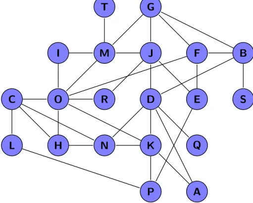
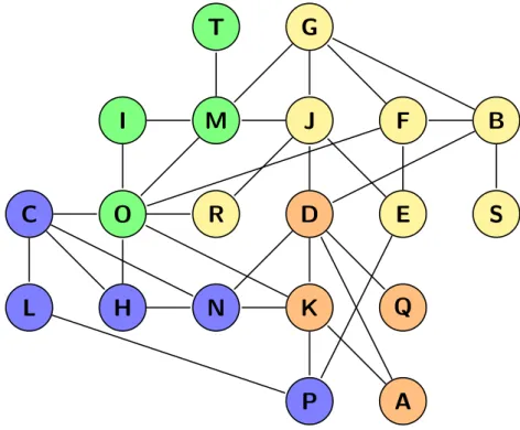
G
Figure 2.1: Example of an undirected graph
2.1.1 Layout
Layouts can be used to rearrange the position of nodes in the graph in such a way that the shape of the graph becomes meaningful. There are multiple algorithms to change the layout of a graph. Some of the algorithms change the graph in a way that they are arranged to show the shape of the graph, others highlight properties of groups of nodes or a single node. We will describe a few of these layout algorithms in this section, to give a glimpse of what is possible.
Circular The circular layout algorithm places all nodes on a circle, with the edges crossing through the circle. This layout is in most cases not very practical, but can be useful for some smaller examples. An example of this layout is given in Figure2.2.
A
B
C
D
E
F
G
Figure 2.2: Example of a graph with circular layout.
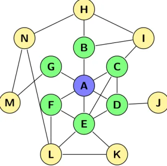
Concentric The concentric layout focuses on a singular node; it places this node in the middle and calculates the shortest path to each of the other nodes. Based on this statistic the nodes are placed on a ring with the value of the shortest path as distance. From this layout, we can easily see which nodes are far away from a particular root node. In Figure2.3, we show aconcentric layout, where node A is the root node. The green nodes are a distance of one away, and the yellow nodes are a distance of two away.
A
B
C
D
E
F
G
H
I
J
K
L
M
N
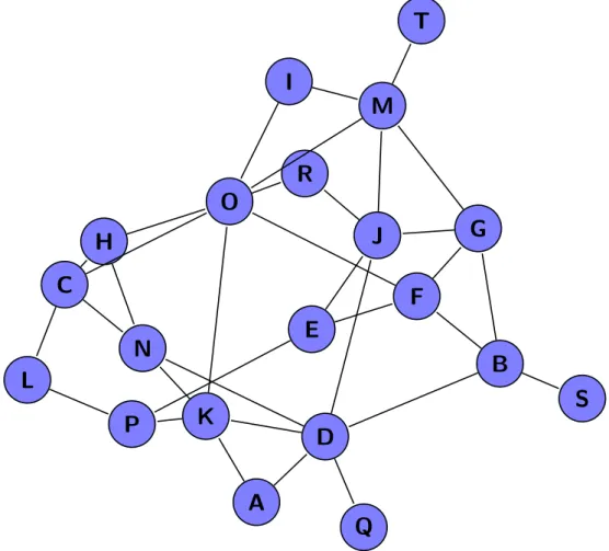
Force atlas The force atlas algorithm is a force-directed algorithm that rearranges the nodes based on repulsion and attraction between nodes. Nodes that have an high weight value between them, will be placed more closely to each other, than nodes with a low or zero weight value between them. By tuning the repulsion strength, we can force the layout of the graph to be more wider. By tuning the attraction strength, we can force the algorithm to place nodes, which, are connected with an high weight value, to place these close to each other. An example of this algorithm is given in Figure2.4, the force atlas layout algorithm is applied to the graph of Figure 2.1.
S
B
G
T
F
M
J
Q
D
E
R
I
A
O
K
N
P
H
C
L
2.1.2 Ranking
Ranking on a graph can be done in many different ways, it can be used to highlight characteristics of nodes or edges of the graph. Ranking on nodes can be done using different statistics, examples of these are: authority, betweenness centrality, closeness centrality,degree,hub andweighted degree. We could also rank the edges of a graph and, for example, use the weight of an edge as ranking statistic.
Example: degree of nodes Below we give an example of the use of ranking as a visualization tool. For this example, we have chosen for the statistic degree as ranking variable. In Figure 2.5we show this ranking for the graph of Figure2.1. We have applied the colors shown in Table 2.1, these colors indicate thedegree of a node, the warmer the color, the higher the degree. Using this visualization, we can see which nodes have the highestdegree and their connections.
A
P
K
N
R
H
M
O
T
Q
C
D
E
I
L
S
J
F
B
G
Figure 2.5: The graph of Figure2.1with ranking applied on the nodes. Ranking is based on the degree of the nodes.
Degree 1 2 3 4 5 7
Color Blue Cyan Green Yellow Orange Red
2.1.3 Partitioning
Partitioning is dividing a graph into clusters. We can use different algorithms to define them; examples of these are the number of triangles, the degree and the modularity. Whereas, the number of triangles stands for the number of triangles where the node part of is.
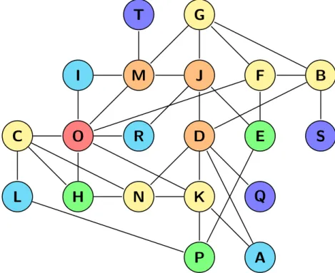
Example: Modularity Below we give an example of the use of partitioning as a visu-alization tool. For this example we have chosen the statisticmodularity as partitioning variable, which is explained in Appendix A. In Figure 2.6, we show this partitioning of the nodes for the graph of Figure 2.1. The distribution of the classes is shown in Table2.2.
A
P
K
N
R
H
M
O
T
Q
C
D
E
I
L
S
J
F
B
G
Figure 2.6: The graph of Figure 2.1with partitioning applied on the nodes.
Parti-tioning is based on the modularity of the nodes.
Class 1 2 3 4
Percentage 25% 20% 35% 20%
2.1.4 Filtering
Filtering is based on keeping and removing nodes and edges, with a particular property or statistic. Some filters are more complex and use the topology of the graph, for example, all nodes with a distance towards the root node less than five.
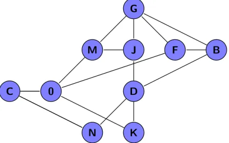
Example: degree filter Below we give an example of the use of filtering as a visu-alization tool. For this example, we have chosen to use the statistic degree as filtering variable. In Figure 2.7 we show this filtering for the graph from Figure 2.1. We have filtered the nodes with a degree higher than three.
K
N
D
J
M
0
C
F
B
G
Figure 2.7: The graph of Figure2.1with filtering applied on the nodes. The applied filter is all nodes with a degree higher than three.
2.1.5 Further reading
For further reading about graph visualization we recommend the following books:
ä Network Graph Analysis and Visualization with Gephiby Ken Cherven [2]
2.2
Graph statistics
Graph statistics are an useful way to get insight in graphs and to compare subgraphs. In this section we will describe the statistics that we will use in our research. We will begin by describing link analysis in Section2.2.1. Next, we will describe cluster analysis in Section2.2.2. At last we will describe classification and graph-based anomaly detection in Sections 2.2.3and 2.2.4, however, these two will not be used in our research.
2.2.1 Link analysis
Link analysis is a graph analysis that uses the edges of a graph. There exist two types of link analysis. The first is the analysis of the nodes by using the edges. The second is the analysis of edges that are highly likely to exist in the future. For example, the suggested friends/ and connections lists from Facebook and LinkedIn.
An example of link analysis is the egocentric network metric. This algorithm looks, until a certain specified depth, at the neighbors of a particular node. This algorithm is particularly useful if already interesting nodes are found; it is then possible to look at nodes that are close to the interesting nodes.
A more complicated algorithm is theHITS (Hyperlink-Induced Topic Search) algorithm, it calculates the importance of a node or its connections in the graph. The HITS
algorithm calculates two scores; the authority score and the hub score. Whereas, a node is called an authority if many hubs, which are also important, are adjacent to it. A hub is the contrary of an authority; a node is called a hub when its connections are important. An extensive description can be found in [4].
2.2.2 Cluster analysis
Cluster analysis is the task of dividing the input data in (overlapping) groups. We differentiate between within-graph clustering and between-graph clustering. In this re-search paper, we will only use within-graph clustering, which is separating the nodes in (overlapping) clusters. Whereas, between-graph clustering is clustering graphs in (overlapping) clusters.
These cluster algorithms can differ a lot from each other, the most important charac-teristics of a cluster algorithm are: Overlapping versus non overlapping; Optimization of connectivity within clusters versus minimization of connectivity between clusters; If there are predefined clusters; And if all nodes are required to belong to a cluster.
An example of a clustering algorithm isHighly connected subgraph clustering. This algo-rithm produces clusters, wherefore; the connectivity within the cluster is high. However, a drawback is that the algorithm is known to create singleton clusters (clusters consisting of one node).
2.2.3 Classification
Classification can be divided into two types of classification, the classification of indi-vidual graphs and the classification of nodes in a graph. Classification is often used in combination with machine learning algorithms, where we use examples to train the algorithm, so we can apply the algorithm to an unclassified dataset. An example would be, where we have a dataset of materials and their properties and we know, which sub-stances are toxic. We could then use this dataset to predict if unknown subsub-stances are toxic or not.
We can use classification for classifying nodes or edges as fraudulent or any other label, as long as we have a train set, which, we can use to train the algorithm, most often with machine learning techniques.
2.2.4 Anomaly detection
Graph-based anomaly detection is the task of finding anomalies in a graph based on the attributes of the nodes, where we differentiate between outliers and in-disguise anomalies. To find outliers, also called ‘white crows,’ we can usecosine similarity, andrandom walks, whereas, the first is not applicable for large graph because of the computing time. For the second, we can use the GBAD algorithm. We will not explain these algorithms further, because these will not be used in our research (see [5]).
2.2.5 Further reading
For further reading about graph statistics we recommend the following book:
ä Practical Graph Mining with R by Nagiza F. Samatova, William Hendrix, John Jenkins, Kanchana Padmanabhan and Arpan Chakraborty [5]
2.3
Graph querying
Graph querying stands for retrieving patterns from a graph. Which patterns are inter-esting depends on the use case. Usually, a domain expert is needed to indicate which patterns could be interesting.
We begin to explain some basic patterns. After that, we describe the NoSQL databases. A form of NoSQL databases is the graph database, this database can be used for graph querying. We focus on this database because we use this database in our research.
2.3.1 Patterns
When we use graph querying, we are looking for patterns. In our case we are looking for strange kinds of relationships between multiple entities, which can indicate possible fraud. By using domain knowledge and using graph visualization to determine patterns, we can query on the database in search for these particular patterns.
C
D
F
E
A
B
C
D
F
E
A
B
C
D
F
E
A
B
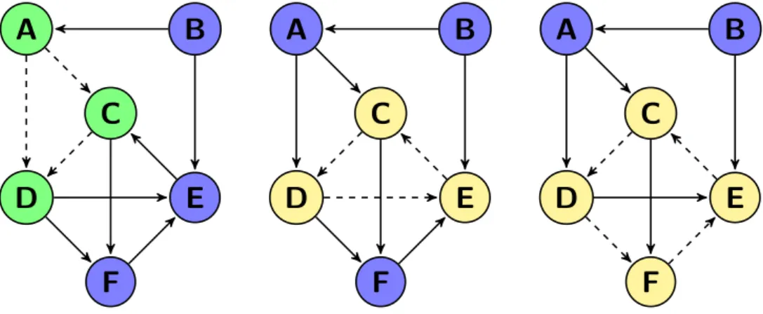
Figure 2.8: Examples of patterns.
In Figure2.8we show three patterns in a graph. In each of the three graphs an example of a pattern is given in green or yellow. The green pattern could be strange if it represents for example leadership roles, where person A is the leader of person C and D, and person C is the leader of person D. This would be strange, because are persons C and D of the same function or has person C an higher function than person D. The yellow patterns could indicate fraud if the edge would mean ‘owner of’, because we would not expect cycles in such a graph.
2.3.2 NoSQL Databases
NoSQL1 stands for ‘Not only SQL’. They are an alternative of traditional relational databases. Compared to relational databases, the advantages can be: Faster data re-trieval; More flexibility; Simpler programming model; And the ability to perform more advanced queries, such as graph queries. However, NoSQL databases are not always the best choice for an application, for example, it can be more difficult to perform a query to select all the rows of a database. Examples of NoSQL databases are: column databases2, key-value stores3, document databases4, and finally, graph databases, which we have used in our research.
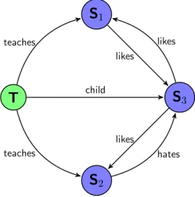
Graph databases Graph databases are databases, where data is represented in graph structures. These graph structures consist of nodes and edges, information of the objects are stored in the nodes, relations and their properties are stored in the edges. If we have, for example, a database with students and teachers, we can model which teachers teach which students and what connections there are between persons, like friendships, family relations or groups. For example, the graph in Figure 2.9could be our graph database.
S
1T
S
2S
3 likes child teaches teaches hates likes likesFigure 2.9: An example of a graph, with a teacher (green) and three students (blue),
where multiple relations exist between them.
The main advantage of graph databases in contrast to other databases is that relations and connections are modeled and queried easily. We can use query languages to search for patterns. If we would use a relational database to search, for example, third-degree friends, we would have to perform multiple joins and would have multiple temporary
1http://en.wikipedia.org/wiki/NoSQL 2 http://en.wikipedia.org/wiki/Column-oriented DBMS 3http://en.wikipedia.org/wiki/Key-value store 4 http://en.wikipedia.org/wiki/Document-oriented database
tables. With a small database, this would not be a big issue, but with a large database (Facebook and LinkedIn networks), this would be disastrous.
2.3.3 Further reading
For further reading about NoSQL, graph databases and graph querying we recommend the following books:
ä NoSQL Distilled, A Brief Guide to the Emerging World of Polyglot Persistenceby Pramodkumar J Sadalage and Martin Fowler [6]
ä Graph Databasesby Ian Robinson, Jim Webber and Emil Eifrem [7]
Related Research
In this chapter we try to give an overview of the research already been done in the fields of graph mining, outlier detection and the Enron email data. This chapter is not an extensive list, we only looked into a selection of the available research. This is based on the articles that we have read, prior to writing this paper.
3.1
Research regarding graph mining
There have been a variety of research studies on the topic of graph mining, treating the topic from several perspectives. Yang and Hwang (2006) [9] propose a data mining framework to detect health care fraud by using the concept of clinical pathways in the form of a network. Clinical pathways are the regular way a patient goes through the process of health care. So, patterns differentiating significantly from a clinical pathway are suspicious.
Subelj, Furlan and Bajec (2011) [10] propose an expert system for the detection of au-tomobile insurance fraud, which uses graphs as the representation of the data. Further-more, they make use of theIterative Assessment Algorithms (IAA)to allocate fraudulent networks.
Jedrzejek, Falkowski and Bak (2009) [11] developed a tool that searches for chain graphs. These graphs can represent flows of money, invoices, goods or services. They target financial crimes that have to use a circular flow of transactions. These circular flows of transactions represent the money that has returned to the fraudulent individual.
3.2
Research regarding outlier detection
The area of outlier detection is very broad. Hodge and Austin (2004) [12] give an overview of outlier detection methodologies in their paper. Some of the techniques they describe are applicable for fraud detection. They partition outlier detection in three types: determining outliers when there is no knowledge about normality and abnormality; model normality and abnormality; model only one of them.
There also exists research on detecting outliers in a graph-based structure. Chakrabarti and Mellon (2004) [13] developed a tool, which uses no parameters, to find clusters in a graph. Furthermore, they propose a novel algorithm to find outliers in the graph and calculate distances between the clusters. The results they achieved were by their words ’excellent and intuitive’.
Also, Shekhar and Zhang (2001) [14] describe algorithms and applications of detecting outliers in a graph. They have tested their algorithms on the Minneapolis-St. Paul (Twin-Cities) traffic dataset. Furthermore, they have compared their results with other clustering methods, and their algorithm provides the best overall performance.
3.3
Research regarding the Enron corpus
A lot of research has been done on the Enron email dataset since it became publicly available in 2002, especially in the first few years following the release. The Enron corpus is unique in its size and its content; there is currently no other corpus available with the same characteristics.
Klimt and Yang (2004) [15] analyze the Enron corpus in their research. They investigate whether the Enron corpus is suitable for email folder prediction. They usesupport vector machines1 as machine learning algorithm to evaluate the suitability of the Enron corpus, furthermore, they also provide a brief analysis of the corpus itself. They also used the CMU dataset, which had similar results to the Enron dataset. In comparison with the CMU dataset the Enron dataset most likely uses more diverse folders.
Chapanond, Krishnamoorthy and Yener (2005) [16] used different filtering methods on the Enron corpus in their research. They filtered the Enron email data based on threshold-based noise filtering and SVD-based noise filtering. Furthermore, they per-formed an analysis to group email addresses similar to each other, and most likely belonging to the same employee. They also did an analysis of the connection of Enron
to the White House, however, after the threshold-based noise filtering and SVD-based noise filtering there was no connection left.
Gloor and Niepel (2004) [17] give an overview of the possibilities of TeCFlow, a tool for temporal visualization and analysis of networks, on the Enron email data. They produce three different analysis, whereas, they start by selecting only the emails with suspicious content and perform an analyses on the resulting network. Second, they use the employees found to allocate more interesting individuals in the total network. At last they create clusters of suspicious activity. Especially, these clusters could be useful in the context of our research.
Experimental Data
In this chapter, we describe the data that we have used and the preparation that we have applied to this data. We have used the email data from Enron, where an enormous fraud was committed and which was revealed in October 2001. These emails were acquired by Federal Energy Regulatory Commission. After their investigation these emails were sold to Andrew McCallum, who released them to researchers.
4.1
Case
Figure 4.1: Enron’s
logo by Paul Rand.
HNG/Internorth merged from Internorth and HNG in 1985 and later became Enron. The former Chief Executive Officer of HNG was Kenneth Lay, he became Chief Executive Officer of Enron only six months after the merger, whereas, Internorth was the larger company. HNG/Internorth was a producer of natural gas and electricity, which was then a regulated market by state. Before working at HNG, Kenneth Lay used to work for the state, where he had been a supporter of deregulated energy markets. When this finally happened, Enron created a business model to buy and sell energy like financial instruments.
Not much later the first Enron scandal was discovered, which involved traders that traded with amounts way above the fixed trading limits. For a long time they expected the price of natural gas to go down, but it only went up. This led to significant losses; they attempted to hide these losses in their books, but were unable to when the losses became too big. That is when the scandal became public.
However, Enron recovered from this scandal, and for a time it went well. Jeffrey skilling was hired initially via McKinsey as Chief Executive Officer of Enron Finance, later promoted to Chief Operation Officer, and Enron became America’s most innovative company for a few years, with many new ideas and large investments. Among other companies, they thought they were in the new age of accounting, and they booked the possible future profits of their ideas.
Only, there was one problem, Jeffrey Skilling’s ideas were creative, but unusual and sometimes questionable financial constructions and accounting principles. The willing-ness to circumvent standard accouting and reporting practices led the firm to hide and take on greater and greater risks. Because of this, it became harder for Enron to look like a profitable company, which it needed to raise the price of their stock and to get loans. Among others, Andrew Fastow, hired by Jeffrey Skilling, created multiple shell company’s to hide their losses and to make it look like if money was coming in.
Eventually, Enron collapsed and declined for bankruptcy on 2 December 2001; it had then approximately 20,000 employees in service. Also, their accountant Arthur Anderson declared bankruptcy, because they did not supervise Enron adequately. The Sarbanes-Oxley Act of 2002 was created after bankruptcy of Enron, WorldCom1 and others. There are various books written about the Enron scandal, like The Smartest Guys in the Room [18], also a well known documentary film, and Enron, the Rise and Fall [19].
4.2
Description
The email data consists of all the emails from Enron employees between 1991 and 2002. For each person, we have all the emails and know to which folder the email belongs. An example of such an email is:
Message - ID : < 1 8 7 8 2 9 8 1 . 1 0 7 5 8 5 5 3 7 8 1 1 0 . J a v a M a i l . e v a n s @ t h y m e > D a t e : Mon , 14 May 2 0 0 1 1 6 : 3 9 : 0 0 -0700 ( PDT ) F r o m : p h i l l i p . a l l e n @ e n r o n . com To : tim . b e l d e n @ e n r o n . com S u b j e c t : Mime - V e r s i o n : 1.0 Content - T y p e : t e x t / p l a i n ; c h a r s e t = us - a s c i i Content - T r a n s f e r - E n c o d i n g : 7 bit X - F r o m : P h i l l i p K A l l e n X - To : Tim B e l d e n < Tim B e l d e n / E n r o n @ E n r o n X G a t e > X - cc : X - bcc : X - F o l d e r : \ P h i l l i p _ A l l e n _ J a n 2 0 0 2 _ 1 \ Allen , P h i l l i p K .\ ’ S e n t M a i l 1 http://en.wikipedia.org/wiki/MCI inc.
X - O r i g i n : Allen - P
X - F i l e N a m e : p a l l e n ( Non - P r i v i l e g e d ). pst
H e r e is our f o r e c a s t
4.3
Preparation
We have used a Java program calledJavaMail2, which was used to format these emails. We use this program to automatically parse the emails and retrieve the sender, the receiver(s), the date and the subject. We have selected all the folders, which indicated sent emails ( sent mail, sent, sent items and sent) to use in our dataset. We assume that by using these folders that we have the complete network of emails sent and received, because what has been sent should also been received. To remove noise from the dataset, we have left out the other email boxes, for example, discussion threads. These emails contain a lot of receivers and, therefore, the connection between the sender and receiver is weak. We have listed the frequently used email boxes in AppendixC.
We have used the email addresses instead of the names for our dataset because these are less prone to typing errors. The four folders that we selected, contained a total of 52,301 emails. However, an email can be sent to multiple receivers, so we created a separate entry in our dataset for each receiver. After this step, we had a total of 82,626 entries. After deduplication by date, subject, sender and receiver, there were 60,226 entries left. Next, we have removed all the emails, wherefore, the receiver was not known, because these would not lead to additional information. After this step, there were 60,083 emails left. Next, we removed all emails, which were to someone outside Enron, which led to a resulting dataset of 45,937 emails. Finally, we removed all the emails, where the sender was equal to the receiver. We ended with a total of 45,781 emails with 5,083 unique email addresses.
The last part is to create a list of nodes and edges from these emails. We have selected all unique email addresses, senders and receivers, and created a list of nodes with these. To create the edges we made a list of all existing combinations of senders and receivers and calculated how many emails there were between the sender and the receiver and given that value as the weight to the edge. The graph that we created now represents the communication network of the emails.
4.4
Characteristics
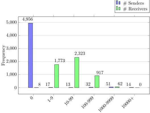
The dataset that we created consists of 5,083 nodes and 10,752 edges. We have created a histogram of the number of emails sent and received for each person, which is shown in Figure4.2. Whereas, the average degree of the graph is equal to 2.12, which is very low for a graph with more than 5000 nodes. Furthermore, the dataset has a range from May, 1991 till June 2002.
0 1-9 10-99 100-999 1000-9999 10000+ 0 1,000 2,000 3,000 4,000 5,000 4,956 17 13 32 51 14 8 1,773 2,323 917 62 0 F requency # Senders # Receivers
Figure 4.2: Histogram of the number of mails sent and received for each individual in
the dataset. Where each bar represents the number of individuals that sent/received a particular number of emails.
Experimental Setup
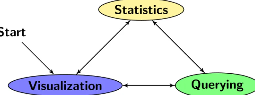
In this chapter, we discuss our experimental setup for each graph mining technique sepa-rately. However, graph mining is not a straight forward process, but an iterative process, as shown in Figure5.1. Furthermore, the start phase is frequently graph visualization, because it is an easy way to get a first feeling with the graph.
Start
Visualization
Statistics
Querying
Figure 5.1: Interaction between the graph mining techniques.
We discuss for each technique the steps that we perform in the analysis. To maintain a readable and scientific structure we divided the analysis of the graph data in experimen-tal setup (this chapter) and the results and the interpretations together in Chapter6. In most of the steps, we use the information that we have found in previous steps. This method was developed iteratively, but is being presented in terms of an experimental framework. We have performed a web search on the individuals that we found to in-dicate whether they are possible fraudulent. Detailed results of this can be found in AppendixD.
5.1
Graph visualization
In this section, we explain how we analyze the graph using visualization techniques. We use the program Gephi to perform the analysis. The values of the parameters are in Table5.1, for the remainder we used the default values. The figures resulting from these steps can be found in Chapter6.
Layout (1)
To get a first impression of the graph, we use the force atlas layout algorithm to rearrange the nodes of the graph. This algorithm creates a layout, where the nodes that are connected are close to each other and vice versa; this is based on the repulsion and attraction strength parameters. We first use a high value for
speed, which, leads to a lower accuracy and then use a low value forspeed, so that we will get close to the optimal structure.
Filtering
The average degree of the graph is only 2.115, therefore, we filter the data to get a more densely connected graph.
Layout (2)
To rearrange the nodes of the filtered graph, we use theforce atlaslayout algorithm, in the same way, as the first step.
Ranking
We use the statisticeigenvector centrality to rank the nodes; the output will be a graph where we can see the most influential nodes in the network.
Partitioning
We use the statistic modularity to create clusters in the graph. Modularity is a measure that calculates the denseness in a cluster and the sparseness between clusters. This way, the distribution of nodes in clusters with the highest value for modularity, will result in a graph with strong interconnectedness and weak between connectedness. Furthermore, we look for visible outliers and the clusters of the individuals found in the previous step.
Technique Algorithm Parameter Value(s)
Layout Force atlas Repulsion strength 100,000
Speed 100 & 1
Filtering Degree range Range [10, max]
5.2
Graph statistics
In this section we explain how we analyze the graph data using statistics techniques. We use the programR to perform the analysis. Furthermore, we use the filtered graph created in graph visualization. Because, some of the algorithms that we use only work on undirected graphs, we created an undirected version.
We perform the techniques of link and cluster analysis from Section 2.2. Moreover, we do not use the techniques of classification and anomaly detection, because we need nodes with attributes, which, are out of scope for this research paper. The used parameters are listed in Table5.2.
Link analysis (1)
We look at the egocentric networks of the individuals with a high eigenvector centrality found with the technique ranking in graph visualization. By extracting these individuals, which, are in both networks we try to indicate more possible fraudulent individuals.
Link analysis (2)
We use theHITS algorithm to allocatehubs andauthorities in the directed graph. These scores indicate important nodes and nodes with important connections.
Cluster analysis (3)
We usehighly connected subgraph clustering algorithm on the undirected graph to find clusters in the graph.
Cluster analysis (4)
We usebetweenness centrality based clustering algorithm on the undirected graph to find clusters in the graph.
Cluster analysis (5)
We use shared nearest neighbor clustering algorithm on the undirected graph to find clusters in the graph.
Technique Algorithm Parameter Value(s)
Link analysis Egocentric network Depth 2
Link analysis HITS Kappa 2
Cluster analysis Highly connected subgraph clustering Kappa 1, 2, 3
Cluster analysis Betweenness centrality based clustering Threshold 0.25, 0.5, 0.75
Cluster analysis Shared nearest neighbor Tau 1, 2, 3
5.3
Graph querying
Because of the scope that we selected for this research paper, namely, only looking at the network itself and not at the content of the emails, we cannot perform graph querying. A more elaborate study could give attributes based on the text in the emails to the nodes. This would create different types of nodes, for which, we could define patterns of interest.
Results and Interpretations
In this chapter we describe the results that we have obtained from the experimental setup (see Chapter5) on the Enron dataset (see Chapter4). We begin with describing the results obtained through graph visualization, followed by the results from the graph statistics. As explained in Chapter5, we will not perform graph querying in this research paper. Note that, not all the steps show interesting results, but we will show them for completeness.
6.1
Graph visualization
Layout (1)
In Figure 6.1the results are shown for using theforce atlas algorithm, with repul-sion strength equal to 100.000. However, the graph is hard to analyze, because it is very dense.
Figure 6.1: Results of graph visualization after adjusting the layout.
Filtering
In Figure 6.2 the results are shown for using the the filter degree range with the range [10, max]. From the original 5,083 nodes and 10,752 edges are 164 (3.23%) nodes and 1,390 (12.93%) edges left. The graph is, therefore, a lot smaller than the previous graph. A lot more edges than nodes are left, therefore, the filtered graph is more connected than the original graph.
Figure 6.2: Results of graph visualization after adjusting filtering on the graph of
Figure6.1.
Layout (2)
In Figure6.3 the results are shown for using the force atlas algorithm, with re-pulsion strength equal to 100.000 on the filtered graph of the previous step. The graph is a lot more organized than the graph of the first step. Therefore, we use this graph for further analysis.
Figure 6.3: Results of graph visualization after adjusting the layout on the graph of
Ranking
In Figure6.4, the results are shown for using ranking with the statisticeigenvector centrality(see Appendix A) on the color and size of the nodes. Whereas, the bigger the node and the warmer its color, the higher the value of eigenvector centrality.
Eigenvector centrality is an important statistic to determine the influence of a node on the network. By finding the most influential nodes in the network, we allocate individuals who standout from the rest.
Figure 6.4: Results of graph visualization after using ranking on the nodes of the
graph in Figure6.3.
In Table6.1 the email addresses are shown, that belong to the five highest values of eigenvector centrality. Furthermore, we have given an indication if they were involved in fraudulent activities concerning Enron. To determine this, we have done a web search. If we found an indication that an individual was involved in fraudulent activities concerning Enron, we have put them on ’Yes’. Furthermore, for the positive cases, we have given a reference in AppendixD.
Email address Eigenvector centrality Fraudulent
1. [email protected] 1.000 Yes
2. [email protected] 0.934 Yes
3. [email protected] 0.696 No
4. [email protected] 0.694 Maybe
5. [email protected] 0.640 No
Table 6.1: Individuals with the highest eigenvalue centrality and an indication if they
Theeigenvector centrality values of Louise Kitchen and John Lavorato differ a lot from the other individuals. Both were most likely involved in fraudulent activities concerning Enron. Also David Delaney, who only scored 0.694, might be involved in fraudulent activities concerning Enron.
Partitioning
In Figure 6.5the results are shown for using partitioning with the statistic modu-larity on the color of the nodes, the size is still determined by the ranking in the previous step. The colors indicate different clusters.
Figure 6.5: Results of graph visualization after using partitioning on the nodes, with the outliers circled, on the graph of Figure6.4.
We can now analyze the nodes of the graph based on three characteristics, the ranking of the nodes, the clusters and the layout. Therefore, we can look at outliers, which can be individuals that appear to be part of a cluster based on their position, but belong to another cluster based on partitioning. We can also look at the large nodes, which indicates a high eigenvector centrality, and look more closely at the cluster to which they belong.
We have allocated three outliers, these are annotated in Figure6.6. The first outlier belongs to the dark blue cluster but lies within the light blue cluster. The second outlier belongs to the red cluster. The nodes from the red cluster lie closely to each other, except this node. The last outlier belongs to the pink cluster, the reason we selected this node as outlier is the same as for the second node, except now for the pink cluster. Regarding the other clusters we did not select other nodes
as outliers. Mainly because multiple nodes of the cluster where spread across the graph.
Louise Kitchen and John Lavorato, the individuals with the highest eigenvalue centrality values from the previous step, both belong to the dark blue cluster. However, the nodes of this cluster are very widespread across the graph, so we do not select any more nodes for further investigation.
Figure 6.6: Results of graph visualization after using partitioning on the nodes, with the outliers circled, on the graph of Figure6.5.
In Table 6.2 the email addresses of the indicated outliers are shown. We found no indication on the web that Geoff Storey or Joe Hartsoe were involved in any fraudulent activities concerning Enron. Furthermore, the second email address does not belong to an individual, it is likely a company service email for the IT group managing email. Thus, this email was likely highly connected because they were sending out notices concerning email service to many users.
Email address Fraudulent
1. [email protected] No
2. [email protected] Not an individual 3. [email protected] Unknown
6.2
Graph statistics
Link analysis (1)
We have created; theegocentric networks, with a depth of two, of Louise Kitchen and John Lavorato, the individuals with the highest values ofeigenvector centrality. There are nineteen individuals, which belong to both egocentric networks. Sally Beck has a strong connection to both Louise Kitchen and John Lavorato, the other eighteen individuals have no strong connection to both. Therefore, there is a large probability that Sally Beck is involved in fraudulent activities.
Email address Louise Kitchen John Lavorato
[email protected] 2 2 [email protected] 2 5 [email protected] 2 4 [email protected] 10 8 [email protected] 2 15 [email protected] 1 1 [email protected] 3 7 [email protected] 1 1 [email protected] 1 1 [email protected] 52 34 [email protected] 1 9 [email protected] 8 4 [email protected] 1 1 [email protected] 2 3 [email protected] 2 10 [email protected] 2 8 [email protected] 4 3 [email protected] 1 1 [email protected] 2 10
Table 6.3: Individuals that both belong to the egocentric network of Louise Kitchen and John Lavorato.
The results are given in Table6.4, we found by web search that Sally Beck was likely involved in fraudulent activities concerning Enron.
Email address Weights Fraudulent
[email protected] 52 and 34 Yes
Table 6.4: Individuals with the strongest connection to both Louise Kitchen and John
Link Analysis (2)
We have used the HITS algorithm on the directed graph with the number of iterations equal to six. The HITS algorithm gives each node an authority and a
hub score. Whereas, the authority score stands for the importance of the node, and thehub score stands for the importance of the connections from that node.
In Tables 6.5and 6.6the results for individuals with the five highestauthority and
hub scores are shown. Furthermore, we show if we found an indication on the web if they were involved in fraudulent activities concerning Enron.
Email address Authority score Fraudulent
1. [email protected] 0.170 No
2. [email protected] 0.138 No
3. [email protected] 0.133 No
4. [email protected] 0.114 Maybe
5. [email protected] 0.112 Yes
Table 6.5: Individuals with the highest authority score and an indication if they were fraudulent.
Email address Hub score Fraudulent
1. [email protected] 0.347 Yes
2. [email protected] 0.319 Unknown
3. [email protected] 0.297 Yes
4. [email protected] 0.272 Yes 5. [email protected] 0.235 No
Table 6.6: Individuals with the highest hub score and an indication if they were
fraudulent.
Of the total of nine individuals we found, we have identified four of them as fraudulent; one as maybe; and for one, we could not find enough information on the web to make an substantiated indication. The remaining three we indicated as non fraudulent. There are more positive results for the hub than for the authority score, which indicates that fraudulent individuals themselves are not very important, but operate from the background.
Cluster Analysis (1)
The highly connected subgraph clustering algorithm withκ equal to one, two and three only detects singleton clusters. Therefore, we cannot conclude anything.
Cluster Analysis (2)
The betweenness centrality based clustering algorithm with the threshold equal to 0.25, 0.5 and 0.75 only detects singleton clusters. Therefore, we cannot conclude anything.
Cluster Analysis (3)
The shared nearest neighbor clustering algorithm with τ equal to one, two and three detects only one large cluster. Therefore, we cannot conclude anything.
Conclusions and Future Research
In this chapter, we first describe the conclusions that we have made, according to our re-search. Furthermore, we discuss the limitations that our research had and opportunities for future research.
7.1
Conclusions
First, we will restate our research question and sub research questions mentioned in Chapter 1.
Can graph mining, consisting of graph visualization, statistics and querying, and their interaction be used in the context of outlier analysis based on a communication
network?
Because we only used graph visualization and statistics, we can only look at these and their interaction. The primary results came from ranking (visualization), partitioning (visualization) and link analysis (statistics).
First we used a filter on the graph, where nodes with a degree less than ten were removed. Secondly, we rearranged the layout of the nodes using a force atlas algorithm. After these preparation steps, we applied ranking on the color and size of the nodes. As a final step, we selected the five individuals with the highest value for eigenvector centrality. From these, we indicated two as fraudulent and one as possible fraudulent after a web search. Next, we used partitioning on the graph with the statisticsmodularity to create clusters. This created a graph, where the size of the nodes was still determined by the ranking, but the color was determined by the partitioning. Furthermore, the layout showed the
repulsion and attraction of the nodes of the traditional network. We indicated three outliers, which lay in another cluster or where relatively far away from the base of the cluster, in the resulting graph. In this case we were unable to find an indication on the web that one of these were fraudulent concerning Enron. Furthermore, one of the nodes was not even a person.
Finally, we have used two types of link analysis. First, we looked at the egocentric networks (with depth two) of Louise Kitchen and John Lavorato and indicated the individuals, who were connected to both. From these individuals we selected Sally Beck, who had a very strong connection to both. After a web search, we indicated her as fraudulent.
The second type of link analysis was the HITS algorithm. We selected the five indi-viduals with the highest authority and the five individuals with the highest hub score, this resulted in nine unique individuals. From these, we indicated four as fraudulent, one as might be fraudulent and one as unknown. The remainder of the individuals we indicated as nonfraudulent. Furthermore, there were more fraudulent individuals from the list of the hub scores than the authority scores.
So, answering our research question, outlier detection using graph mining on a commu-nication network can certainly be done given our results. In total we did a web search on eighteen individuals, we indicated nine of them as possible fraudulent. However, still more research is needed to take into account classification and anomaly detection from graph statistics, and graph querying. Furthermore, the techniques should be tested on other datasets to verify our results.
7.2
Limitations
Because we had only limited time (one month) to perform this research, our research has some limitations. We selected the scope only to look at the network itself and not at the content of the emails. Therefore, we disregarded a substantial amount of information. Furthermore, this paper is focussed on researching outlier detection using graph mining specifically on the Enron email dataset. Therefore, we can only give an indication of the quality and effectiveness of the graph mining techniques on outlier detection.
At last, we have done a web search to indicate if individuals are fraudulent concerning Enron. However, these indications do not have to be true. Furthermore, we found too little information for some of the individuals to make an indication.
7.3
Future research
We have researched a small part of the possibilities of outlier detection using graph mining. Therefore, there are a lot of opportunities to follow up and extend this research. First, we have calculated the weight between two individuals as the number of emails between them. However, emails that are send from one individual to another are in most cases more valuable than from one individual to many individuals. It would be more advanced, when we take the importance of the sender into account; we would then get an algorithm similar to Google Pagerank.
Furthermore, we have only looked at the network itself while there is a major amount of information available in the emails. We could, for example, create attributes for the nodes based on a keyword search in the emails on relevant words.
However, we could also create or use if available reference material from other networks with fraudulent activities. With this reference material, we could use classification to classify if a network or its nodes are fraudulent. It will be necessary for the nodes to have attributes because only classifying on the network itself is not possible if there are not different types of nodes.
Moreover, we have now tested the graph mining techniques only on the Enron email dataset. This makes our research limited, however, further research could be done on other datasets.
Lastly, there also exist programs, which, can show the evolving graph over time. For our case this could be done on the basis of the send date in the emails. This way, the beginning of a scheme can be spotted, and outliers over time can be found.
Terminology
In this appendix, we describe the commonly used terminology in the field of graphs. Graphs consist of two types of objects, namely nodes and edges. Whereas, nodes repre-sent entities, which can be persons, company’s, addresses, etc. Edges reprerepre-sent relations, which can reach from family relations to company ownership. There are two types of edges, undirected and directed. Undirected edges indicate that the two nodes stand equal in the relation, whereas, with directed edges this does not have to be the case. In FiguresA.1 andA.2 two graphs are shown, on the left an undirected graph and on the right a directed graph.
B
D
G
F
H
E
A
C
Figure A.1: Example of a undirected
graph.
B
D
G
F
H
E
A
C
Figure A.2: Example of a directed
graph.
Simple graphs A simple graph is a graph of which its edges are undirected and where between each pair of nodes there exist at most one edge. Furthermore, in a simple graph there are no self-loops, which are edges that start and end at the same node.
Connected graphs A connected graph is a graph, where each node can be reached from all the other nodes. In other words, there exists a path between all nodes. If there are nodes with no connections, we call them isolated nodes.
Modularity Modularity is a measure that can be applied to a graph divided into clusters. It indicates the number of edges that fall within a particular cluster compared to the number of edges that would fall within that cluster if the edges were randomly distributed. A more precise definition is given at1.
Eigenvector centrality Eigenvector centrality is a relative measure that calculates the influence of the node on the graph. It is not a measure of direct centrality, but a measure of being highly connected to nodes with high centrality. This statistic is used by the PageRank algorithm at Google2.
Spanning tree A spanning tree is a subgraph of a graph, which includes all the nodes of the original graph and some (or all) of its edges, such that the new subgraph becomes a tree. Furthermore, in a spanning tree all nodes are reachable, in other words, a spanning tree is connected.
Authority and hub An authority node is a node, which is referenced by many dif-ferent hubs, nodes with a high hub score. Whereas, ahub node is a node with valuable connections to other nodes. A more precise definition is given at3.
Betweenness centrality Betweenness centralityis a relative measure of the centrality of a node in the networks. In other words, it calculates the percentage of shortest paths between all nodes that go through the node. A more precise definition is given at4.
Degree The degree of a node in an undirected graph is equal to the number of edges adjacent to it. In a directed graph, we make a distinction between in-degree and out-degree. The in-degree of a node is equal to the number of edges, which end at this node. Whereas, the out-degree of a node is given by the number of edges, which start at this node. In FiguresA.1 and A.2, A is an unconnected node and nodes F and H are leaf nodes. This corresponds to the degree of zero and one in Table A.1.
1http://en.wikipedia.org/wiki/Modularity (networks) 2 http://www.math.cornell.edu/ mec/Winter2009/RalucaRemus/Lecture3/lecture3.html 3http://www.math.cornell.edu/ mec/Winter2009/RalucaRemus/Lecture4/lecture4.html 4 http://en.wikipedia.org/wiki/Betweenness centrality
Node A B C D E F G H
Degree 0 2 2 3 2 1 5 1
In-degree 0 0 0 2 2 1 2 1
Out-degree 0 2 2 1 0 0 3 0
Table A.1: Degree, In-degree and Out-degree of the graphs in FiguresA.1andA.2.
We can also calculate the averagedegree of a graph, which is equal to the total degree di-vided by the number of nodes. For the undirected and directed graph in Figures A.1and A.2, this is respectively equal to 2.0 and 1.0.
Tools
In this appendix, we will describe three tools, which can be used for analysis, for each of the graph mining techniques.
B.1
Graph visualization
In this section, we describe a few of the graph visualization tools that are available and that could be used for graph visualization (see Section2.1). For each graph visualization tool we show an example in FigureB.1.
Gephi1 Gephi is a graph visualization tool that allows users to explore and under-stand graphs. The user can drag and replace the nodes, but also to use algorithms to rearrange all the nodes. Gephi allows the user to use different statistics to highlight certain characteristics of the graph. Furthermore, it allows the user to look at a subset of the graph.
GraphML2 GraphML is a graph visualization tool, with its primary focus on the layout of the graph. Compared to Gephi, it is less based on graph statistics. It uses a language core to let the user describe the structure of the graph.
Walrus3 Walrus is a graph visualization tool that can visualize large directed graphs in 3D space. The layout is applied by using an user supplied spanning tree (see AppendixA). 1 www.gephi.org 2 www.graphml.graphdrawing.org 3 www.caida.org/tools/visualization/walrus 40
(a)Gephi (b) GraphML (c) Walrus Figure B.1: Examples of graph visualization tools.
B.2
Graph statistics
In this section, we describe a few of the statistical tools available for graph statistics (see Section2.2).
R4 R is a statistical language based on the language S, which was originally developed for statisticians. R provides a wide range of statistical and graphical techniques. Fur-thermore, R has an extensive community contributing to new and consisting packages.
SPSS5 SPSS is a statistical tool widely used in the area of social science. SPSS pro-vides, among others, descriptive statistics, bivariate statistics and prediction for identi-fying clusters.
SAS6 SAS, which stands for Statistical Analysis System, is a software tool for advanced
analytics, business intelligence, data management, and predictive analytics. In 2010, a social media analytics product was added to the software.
B.3
Graph querying
In this section, we describe a few of the graph databases that are available and that could be used for graph querying (see Section2.3).
Neo4j7 Neo4j is a full native graph database, meaning that its graph processing, and storing are both done in graphs. Furthermore, Neo4j is an open-source database imple-mented in Java and supports many programming languages.
4 www.r-project.org 5 www-01.ibm.com/software/analytics/spss 6 www.sas.com 7 www.neo4j.org
Titan8 Titan is a partial native graph database, meaning that its graph processing is done in graphs, but its storage is done in a transactional database. Titan supports thousands of concurrent users working on the same graph.
OrientDB9 OrientDB is a product from Oracle and is a full native graph database written in Java, meaning that it’s graph processing and storing are both done in graphs. It is a document-based database, with direct connections between documents. Next to graph query languages, it also supports standard SQL.
8www.thinkaurelius.github.io/titan 9
Mailboxes
Below we give an overview of the mailboxes found in the Enron dataset. We have se-lected the mailboxes, which were held by more than ten employees, or that had ‘sent’ in the name. For each mailbox, we have calculated the number of employees who used this folder and the number of emails in these folders.
Mailbox Number of employees Number of mails
deleted items 70 23.363 inbox 70 23.154 sent items 70 14.763 all documents 61 47.850 discussion threads 51 29.700 sent 48 22.294 notes inbox 42 9.981 sent mail 40 1.4981 calendar 37 999 contacts 27 278 personal 20 1.150 tasks 17 45 to do 16 162 sent 2 263
Table C.1: Mailboxes present in the Enron dataset.
Fraudulent References
Employee Description Reference
Louise Kitchen
Louise Kitchen received the second largest bonus of two million dollar, days before Enron filed for bankruptcy.
http://www.salon.com/2002/ 02/08/enron bonuses/
Louise Kitchen was one of the creators of Enron Online, Enron linked itself to every buyer and seller.
http://news.bbc.co.uk/2/hi/ business/1684503.stm
John Lavorato
John Lavorato received the largest bonus of five million dollar, days before Enron filed for bankruptcy.
http://www.salon.com/2002/ 02/08/enron bonuses/ http://usatoday30.usatoday.com/ money/industries/energy/2005-02-03-enron x.htm David Delaney
David Delaney testified against Enron to implicate Jeffrey Skilling, by claiming they discussed possible illegal transactions.
http://www.npr.org/templates/ story/story.php?storyId=5241749
Sally Beck
Sally Beck received a bonus of $ 350,000 days before Enron filed for bankruptcy.
http://edition.cnn.com/2002/ LAW/02/09/enron.bonuses/
James Derrick
James Derrick was Enron’s general counsel and most likely knew about the accounting scandals.
http://www.nytimes.com/2006/04/
07/business/businessspe-cial3/07enron.html? r=0
Rick Buy
Rick Buy was confronted by Mr. Kaminski about too large risks using LJM to hedge, but ignored him.
http://www.nytimes.com/2006/03/
15/business/businessspe-cial3/15enron.html
Table D.1: Employees and their functions of Enron (1).
Employee Description Reference
Mark Haedicke
Mark Haedicke was informed about the controversial shell companies.
http://www.salon.com/2002/02/ 08/enron bonuses/
Richard Sanders
Richard Sanders knew about Enron’s manipulative trading practices.
http://www.cantwell.senate.gov/
public/index.cfm/press- releases?ID=9323d158-bfda-4b28-978d-8f35e488ada9
[1] Maarten van Steen.Graph Theory and Complex Networks An Introduction. Maarten van Steen, April 2010.
[2] Ken Cherven. Network Graph Analysis and Visualization with Gephi. Packt Pub-lishing Ltd., September 2013.
[3] Scott Murray. Interactive Data Visualization for the Web. O’Reilly, March 2013.
[4] Sergey Brin and Lawrence Page. The anatomy of a large-scale hypertextual web search engine. Computer networks and ISDN systems, 30(1):107–117, 1998.
[5] John Jenkins Kanchana Padmanabhan Nagiza F. Samatova, William Hendrix and Arpan Chakraborty. Practical Graph Mining with R. Chapman and Hall/CRC, July 2010.
[6] Pramodkumar J. Sadalage and Martin Fowler. NoSQL Distilled, A Brief Guide to the Emerging World of Polyglot Persistence. Addison-Wesley, 2013.
[7] Ian Robinson, Jim Webber, and Emil Eifrem. Graph Databases. O’Reilly, June 2013.
[8] David Montag Michael Hunger and Andreas Kolleger. Good Relationships. C4Media, 2010.
[9] Wan-Shiou Yang and San-Yih Hwang. A process-mining framework for the detec-tion of healthcare fraud and abuse. Expert Systems with Applications, 31(1):56–68, 2006.
[10] Lovro ˇSubelj, ˇStefan Furlan, and Marko Bajec. An expert system for detecting automobile insurance fraud using social network analysis. Expert Systems with Applications, 38(1):1039–1052, 2011.
[11] Czeslaw Jedrzejek, J Bak, and M Falkowski. Graph mining for detection of a large class of financial crimes. In17th International Conference on Conceptual Structures, Moscow, Russia, 2009.