Catering through Nominal Share Prices
MALCOLM BAKER, ROBIN GREENWOOD, and JEFFREY WURGLER∗
ABSTRACT
We propose and test a catering theory of nominal stock prices. The theory predicts that when investors place higher valuations on low-price firms, managers respond by supplying shares at lower price levels, and vice versa. We confirm these predictions in time-series and firm-level data using several measures of time-varying catering incentives. More generally, the results provide unusually clean evidence that catering inf luences corporate decisions, because the process of targeting nominal share prices is not well explained by alternative theories.
IN FRICTIONLESS AND EFFICIENTstock markets, there is no optimal nominal
(per-share) stock price. A firm’s board of directors may choose to split to manage the nominal share price and number of shares outstanding but cannot change its overall market value through these means. Yet boards typically do manage their firms’ nominal share price, rather than watch it passively drift with re-turns. Theories offered to explain share price management include arguments that trading costs depend on nominal prices (Dolley (1933), Angel (1997)), that splits signal inside information (Brennan and Copeland (1988), Asquith, Healy, and Palepu (1989), and Ikenberry, Rankine, and Stice (1996)), or that prices in certain ranges simply constitute a market norm from which there is little gain to deviating (Rozeff (1998), Weld et al. (2009)).
In this paper we propose a catering theory of nominal share prices. We de-fine catering as the managerial behavior of increasing the supply of a char-acteristic that investors appear to be paying a premium for, even though that characteristic does not increase fundamental value. The catering the-ory of nominal share prices thus posits that the supply of securities of dif-ferent price ranges is partly a response to investor demand for securities of different price ranges: Managers increase the supply of low-priced securities
∗Baker and Greenwood are at the Harvard Business School and National Bureau of Economic
Research and Wurgler is at the NYU Stern School of Business and the National Bureau of Eco-nomic Research. For helpful comments, we thank Yakov Amihud; Lauren Cohen; Ken French; Sam Hanson; Harrison Hong; Byoung-Hyoun Hwang; Eric Kelley; Owen Lamont; Ulrike Malmendier; Ashwin Malshe; Jay Ritter; Andrei Shleifer; Erik Stafford; Dick Thaler; and seminar participants at the American Finance Association, Arizona State, Copenhagen Business School, Dartmouth, Helsinki School of Economics, Kellogg, the NBER Behavioral Finance conference, the Norwegian School of Management, NYU Stern, Penn State, Stockholm School of Economics, SUNY Bingham-ton, the University of Arizona, the University of Florida, and the University of North Carolina. We thank Jay Ritter for providing data. Baker and Greenwood gratefully acknowledge financial support from the Division of Research of the Harvard Business School.
when investors are paying a premium for them. Empirically, this theory pre-dicts that splits will be more frequent, and to lower prices, when the val-uations of low-priced firms are attractive relative to those of high-priced firms.
To explain managerial behavior, the catering theory requires only that man-agers believe that nominal prices matter to investors. The majority of manman-agers subscribe to this belief (Baker and Gallagher (1980)), but the theory gains fur-ther motivation from evidence that, contrary to efficient markets, key return characteristics in fact are affected by nominal price. Green and Hwang (2009) find that stocks that split experience sudden increases in their comovement with lower-priced stocks. Ohlson and Penman (1985) find that stocks that split experience large increases in volatility; thus, as splitting stocks comove more with lower-priced and generally smaller-cap stocks, they inherit these stocks’ higher volatility as well. Lakonishok, Shleifer, and Vishny (1992) and Gompers and Metrick (2001) show that individual investors hold lower-priced stocks than institutions, suggesting a segmented market, and Schultz (2000) shows that the number of small shareholders increases following a split. Black (1986) also views low-price stocks as subject to greater noise trading. Investors thus appear to categorize stocks in part based on price, and this affects returns, much as the addition or deletion of a stock from an index affects returns in Barberis, Shleifer, and Wurgler (2005), Greenwood (2008), and Greenwood and Sosner (2007).
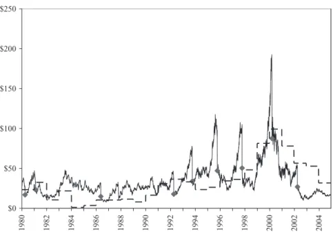
An example introduces our main ideas. Figure 1 plots the share price of Ap-plied Materials, Inc. from 1980 through 2004. ApAp-plied Materials enjoyed success in this period and split its shares nine times. However, far from maintaining a constant share price, the company split to nine different prices, ranging from $15 to $88, through both 2-for-1 and 3-for-2 splits. Catering predicts splits to lower prices when lower-priced shares are in favor. Consistent with this predic-tion, the figure illustrates a close connection between the post-split share price and a relative valuation measure that we refer to as the “low-price premium,” the log difference between the average market-to-book ratio of low-nominal-price firms and that of high-nominal-low-nominal-price firms. In the figure, the series is inverted so that higher values suggest an investor preference for higher-priced stocks. Simply put, the figure shows that when low-priced stocks enjoyed rela-tively high valuations, Applied Materials maintained a lower share price, and when high-priced stocks enjoyed high valuations, it maintained a higher share price.
Our empirical work employs three time-series proxies for catering incentives. The first is the low-price premium. The second is based on the strong cross-sectional relationship between size and share price (Dyl and Elliott (2006) and Weld et al. (2009)), which suggests the possibility that catering-minded split-ters may be trying to portray themselves not as low-priced firms per se but rather as small-cap firms. We therefore construct a “small-stock premium” as the average market-to-book ratio on small-cap firms relative to the average market-to-book ratio on large-cap firms. The third measure of the time-varying incentive to reduce prices is the average announcement effect of recent splits.
$0 $50 $100 $150 $200 $250 1980 1982 1984 1986 1988 1990 1992 1994 1996 1998 2000 2002 2004
Figure 1. Stock splits by Applied Materials, Inc. Applied Materials’ monthly share price (solid) is plotted against the low-price premium (dash—scale adjusted and inverted). Applied Ma-terials went public in the fourth quarter of 1972, split its stock for the first time in the second quarter of 1980, and split eight more times through 2004. Diamonds indicate split dates and mark the post-split price. We omit the scale of the inverted low-price premium.
Greenwood (2009) finds that high announcement effects for Japanese splitters are associated with more splits and higher split ratios in subsequent quarters, results consistent with catering.
An accounting framework for nominal share prices suggests examining four components of publicly traded firms’ “price management” decisions. These are the initial price chosen at the IPO; the binary decision to split in a given period; the price chosen by splitters; and, summarizing the combined effect of the latter two decisions, the average change in price due to price management in a given
period.1 Using both time-series and firm-level data, we examine how each of
these components of price management is affected by catering incentives. We find strong empirical support for the catering predictions. In terms of univariate time-series regressions, our proxies for catering incentives explain up to 30% of the annual variation in the frequency of stock splits, with more firms splitting when low-priced or small-cap firms have higher valuations. The average decline in price across firms, including the net effect of all splits, stock
1To be clear, Weld et al. (2009) emphasize that stock prices are quite stable relative to the
extreme benchmark of no price management. However, relative to the other extreme benchmark of constant nominal price levels, prices are quite variable over time. The average prices selected by stocks that split, the average prices selected by IPOs, and average nominal stock prices in general have varied by a factor of 2 to 3 over the last few decades. We address this variation.
dividends, and reverse splits, is also larger when investors favor lower-priced firms. Of course, prices are ultimately what we seek to explain. Catering in-centives explain up to 75% of the time variation in (log) IPO offer prices and 78% of the time variation in (log) first-day closing prices, with firms going pub-lic at higher prices when catering incentives point in that direction. Perhaps most broadly, catering proxies also explain up to 52% of the time variation in (log) post-split prices chosen by splitters. Theories based on transaction costs or asymmetric information are unlikely to achieve this explanatory power. The effects are robust to controlling for other determinants of splits such as overall average prices and recent returns.
We consider several robustness tests for the regressions involving post-split prices, such as subsample splits, time trends, difference specifications, and so forth, with little qualitative change in the results. One interesting finding that emerges is that catering incentives affect post-split prices only for larger firms. That is, the post-split price results ref lect large firms trying to “act small” at opportune times, not small firms acting large. However, the results for IPO prices involve smaller, younger firms, so in that sense firms respond to catering concerns at multiple points in their life cycle. We also conduct robustness tests using firm-level data. This controls for changes in the composition of firms that might confound aggregate time-series tests. We find that proxies for catering incentives have incremental explanatory power for the various components of price management when examined at the firm level, after controlling for firm-and industry-level characteristics.
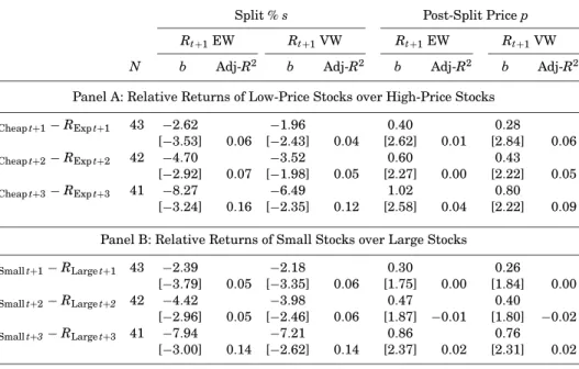
Our final tests involve future stock returns. As noted above, it is not required that share prices be inefficient in order for catering to explain managerial be-havior. Managers may cater in vain to an efficient market, not understanding that the valuations of low- and high-priced stocks differ for fundamental rea-sons. Nonetheless, we treat subsequent stock returns as proxies for the correc-tion of ex ante mispricing and ask whether observed split patterns are consis-tent with the successful pursuit of misvaluation. Perhaps surprisingly, given our relatively short time series, the evidence is consistent with this view. High split frequencies and low post-split prices portend lower future returns on small stocks versus large stocks and on low-priced stocks versus high-priced stocks.
In summary, nominal share prices are inf luenced by catering incentives: There is a supply response to demand shifts. One question that the results raise, and that we leave to future work, is why nominal share prices matter to investors. Institutional trading frictions may play a role. The psychology of stock price levels is unexplored. Weld et al. (2009) suggest that stock prices con-stitute a norm. Perhaps some investors suffer from a nominal illusion in which they perceive that a stock is cheaper after a split, has more “room to grow” ($10 is farther from infinity than is $25), or has “less to lose” ($10 is closer to zero than is $25). Alternatively, perhaps they naively equate low nominal prices with small capitalization. Given the strong cross-sectional correlation between price and capitalization, and the fact that for individual investors it is a bit harder to obtain capitalization data than a price quote, this is not an entirely unreasonable heuristic. Managers of large caps may be able to exploit it. More generally, investors may categorize stocks according to price so that a change
in price can potentially lead to an increase in attention or investor recognition in the sense of Merton (1987). Equivalently, clienteles with a particular focus
in terms of stock price may shift in importance over time.2Whatever the
mech-anism, our particular results suggest time variation. Occasionally, investors as a group shift focus to different price categories and professional arbitrageurs are unable to fully accommodate these demands, leaving room for firms to help
fill the gap.3In some respects, firms are well-positioned to engage in this type
of arbitrage.4
The results make two contributions. First, they support a new theory of why firms split. In doing so they add nominal share prices to a list of managerial
decisions that are inf luenced by catering considerations.5Baker and Wurgler
(2004a, 2004b) and Li and Lie (2006) consider catering via dividend policy. Cooper, Dimitrov, and Rau (2001) and Cooper, et al. (2004) find that corporate names, for example “Pets.com” versus “Pets, Inc.,” can be shaped by catering considerations. In addition, Greenwood (2009) finds that firms in Japan are more likely to split following a period when other splits have generated high
announcement returns,6 Polk and Sapienza (2009) suggest that corporate
in-vestment decisions are shaped by catering considerations, Aghion and Stein (2008) view them as an inf luence on the strategic decision to cut costs or max-imize sales growth; and Baker, Ruback, and Wurgler (2007) suggest that time-varying investor preferences for the conglomerate form may help to explain the rise and subsequent dismantling of conglomerates. A second contribution is that nominal share prices and stock splits offer a cleaner test of catering than many settings considered in prior work. This is because nominal share prices and stock splits (not “settings”) are not associated with any confounding, “real” motivation involving firm fundamentals.
The paper proceeds as follows. Section I outlines the methodology and main hypotheses. Section II presents time-series tests. Section III offers firm-level tests. Section IV examines return predictability. Section V concludes.
2Odean (1999), Hirshleifer and Teoh (2002), and Barber and Odean (2008) emphasize that
individual investors as a group limit their search for stocks to those that catch their attention. Nominal prices and splits may play a role in attracting individual investor attention, and thus stimulating demand.
3See Bikhchandani, Hirshleifer, and Welch (1992) for a model of fads and customs.
4Baker, Ruback, and Wurgler (2007) describe the case of an overpriced firm taking advantage by
issuing equity. If the equity subsequently appreciates, investors are unlikely to complain, whereas a hedge fund that shorts the overpriced firm is in a far worse position. Analogously, a firm that splits because it perceives low-nominal price firms to be overvalued is not going to be criticized by its investors if the low-price premium subsequently widens, but a hedge fund that shorts low-priced firms will suffer obvious losses. Greenwood, Hanson, and Stein (2009) argue that compared with hedge funds, firms are better suited to accommodating supply and demand shocks.
5Somewhat related, Hong, Wang, and Yu (2008) suggest that firms can directly inf luence the
supply and demand conditions in their own securities by repurchasing shares.
6The mechanism in Greenwood’s paper is different from what we study here. In Greenwood’s
paper, a split generates investor demand (or short covering) not through its effect on nominal prices but rather through its effect on the quantity of tradeable shares. This is not catering in the sense of providing a greater supply of securities that are in demand. However, the pattern that time-varying announcement effects produce a corporate response is similar.
I. Methodology
Stock prices change passively with stock returns and actively through price management. Price management has several components. We start by introduc-ing a general accountintroduc-ing framework for price management and then describe the main hypotheses involving catering.
A. Accounting for Share Prices
Stock prices are initially set at the IPO. Subsequently, active price setting happens through the choice of how often to split and at what ratio. Ignoring
dividends for the moment, stock prices are determined as follows. Prices P
typically grow by the stock returnR. The manager of firmican lower or raise
the end-of-period price by choosing to split the stock:
Pi,t=Pi,t−1·(1+Ri,t)·(1+Si,t·Ni,t), (1)
where S is an indicator variable, equal to one if the manager decides to
split the stock, and N is the inverse of the split ratio minus one. For
exam-ple, in a typical 2-for-1 stock split, N (and hence SN) is equal to −0.5; in
a 100-for-1 split, N (and SN) equals −0.99. We can express this in logs as
follows:
pi,t= pi,t−1+ri,t+log(1+Si,t·Ni,t)≡pi,t−1+ri,t+mi,t ≈pi,t−1+ri,t+si,tn,
(2)
where p is the log price, ris the log total return, and m is the net effect of
splitting activity between timetandt+1. If the split ratio, and thereforeN,
does not vary over time—this is approximately the case empirically—thensis
simply an indicator variable for splits,nis a constant equal to the log of 1+N,
and the approximation in equation (2) is exact.
In addition to the explicit effect of splitting throughs andn, the manager
is implicitly controllingpthrough splitting decisions in prior periods. In that
spirit, we can substitute forpi,t−1:
pi,t ≈ Ti
k=0
ri,t−k+si,t−kn+pi,IPO, (3)
whereTis the number of periods since firmi’s IPO.
Dividend policy can be treated in one of two ways. It can be lumped into active price selection by using total returns in the equations above or it can be taken as exogenous by using only the capital gains portion of returns in the equations above. We take the latter approach, focusing on the role of splits.
Our focus in the empirical tests is on the aggregate determinantsxand, to a
lesser extent, the firm-level determinantswof active price selection. We take
four specifications. In each case, we look at firm-level and market-wide data. The initial measure of price selection is the IPO price:
pi,IPO= f(wi,IPO,xt−1)+ui,IPO or, at the market level,pt,IPO= f(xt−1)+ut.
(4) The narrowest measure of price selection following the IPO is simply the
indicator variables:
si,t= f(wi,t−1,xt−1)+ui,torst= f(xt−1)+ut. (5)
We then expand this to include the combined effect ofsandn:
mi,t= pi,t−pi,t−1−ri,t = f(wi,t−1,xt−1)+ui,t ormt= f(xt−1)+ut. (6) The broadest measure of price selection is the price level itself:
pi,t= f Ti k=0 ri,t−k,wi,t−1,xt−1 +ui,t or pt = f T k=0 rt−k,xt−1 +ut. (7) For the IPO price, we of course focus on firms that have just listed. For the
price level, we focus in similar spirit on firms that have split in periodt. These
firms have made an active decision within period t so the price ref lects an
explicit choice, rather than simply managerial inertia. We also include past returns and price levels in these specifications. For tests of the frequency of splits and their combined effect on prices, we can include all listed firms.
B. Main Hypotheses
When estimating these four equations, we are particularly interested in the
effect of elements ofx that proxy for catering incentives. In particular, when
the valuations of low-priced or small-cap firms are high relative to other firms, catering implies that prices in (4) and (7) will be lower, all else equal. With re-spect to equations (5) and (6), we hypothesize that when the relative valuations of low-priced or small-cap firms are high, splits will be more common and lead, on average, to greater reductions in share prices.
The last hypothesis we test is complementary but somewhat distinct. We consider future returns on low-priced and small-cap firms (relative to other
firms) as a dependent variable, putting split frequencysand post-split pricesp
on the right-hand side as predictors. The idea is that if mispricing indeed causes splits toward a particular price range, we may observe return predictability on stocks in that price range as their mispricing subsequently corrects.
II. Time-Series Tests
We begin with time-series tests involving average or aggregate measures of active nominal price management such as average post-split stock prices, average prices chosen by newly public firms, and aggregate split frequencies of
listed firms. This is a natural level of analysis because our proxies for catering incentives are time-series measures.
A. Data on Splitting Activity and Post-split Prices
We track stock splits and post-split prices for all shares on CRSP between 1963 through 2006 that have share codes of 10 or 11. Stock splits are events with a CRSP distribution code of 5523. We distinguish between three types of splits. Regular splits are defined as events having a split ratio of greater than 1.25-for-1. Stock dividends have split ratios between 1.01-for-1 and 1.25-for-1. Reverse splits have split ratios less than 1-for-1.
The first several columns of Table I report the total number of splits, the average pre-split price, the average post-split price for splitters, and the
aggre-gate effect of price management (which we labelm). The pre-split price is the
closing price on the day prior to the split. The post-split price is the pre-split
price divided by the split ratio. The broader measure of splitting activity m
measures the average active price management over the course of the year. It is the average across all listed firms of the log difference between the actual stock price and the beginning-of-year stock price grown at the stock return
ex-cluding dividends. For example, in 1963 the average is−4.00%, meaning that
the average firm reduced its price by 4% through splitting activity. The last two columns show the average first-day and offering prices for IPOs. We thank Jay Ritter for providing IPO dates, offer prices, and midpoint of the pre-IPO filing range prices; the first-day prices are from CRSP. We note that the Penny Stock Reform Act of 1990 places restrictions on IPOs that are priced below $5, which is at least one reason why we see average IPO prices never dropping below $11 after 1990.
A salient feature of Table I is that the fraction of firms that split varies con-siderably over time. In 1970, for example, 46 regular splits were conducted, or fewer than 2% of listed firms, while in 1983, 780 regular splits were con-ducted, meaning well over 10% of listed firms split. (Note that Table I counts the number of splits, not the number of firms that split. However, it is rare for a firm to split more than once in a year, so the number of splits is close to the number of firms that split.) The broader measure of price management also varies over time, from a maximum reduction in price of 8.69% in 1981 to
an increase in price of 0.32% in 2001.7To some extent these series are driven
by returns. When past returns are high, managers tend to move prices down toward their historical trading range, consistent with the norms theory of Weld et al. (2009).
The “target” prices to which splitters split and the prices at which newly public firms choose to list vary greatly over time. Shedding light on these target prices is our primary goal. At the height of the Internet bubble, the average post-split price approached $50 per share, whereas in earlier years it had been as low
7During 2001, there were numerous reverse splits by stocks that were in danger of being deleted
Table I
Stock Splits and Post-split Prices
This table presents the number of splits, the average pre-split price, the average post-split price, and the average split ratio for splits, stock dividends, and reverse splits. Events with a CRSP distribution code of 5523 are divided into three categories: Splits have a split ratio greater than 1.25-for-1; stock dividends have a split ratio between 1.01-for-1 and 1.25-for-1; and reverse splits have a split ratio less than 1-for-1. The pre-split price is the closing price on the day prior to the split. The post-split price is the pre-split price times the reciprocal of the split ratio. The left-most column lists the year-end sample of CRSP firms.
The right-most columns show a summary measure of splitting activitymand the average offering price,
first-day close, and midpoint for the pre-IPO filing range for IPOs.mis equal to the log of the ratio of
the actual average stock price to the beginning-of-year stock price grown at the stock return excluding
dividends, expressed in percentage terms. We report the equal-weighted averagemacross all listed stocks.
Splits Stock Dividends Reverse Splits IPO Prices
Year All N Pre Post N Pre Post N Pre Post m% Close Offer Mid File
1963 2,074 57 63.96 32.49 2 34.50 27.60 5 2.59 10.94 −4.00 1964 2,138 99 70.12 32.78 13 82.85 66.28 10 3.10 9.07 −3.62 1965 2,135 132 72.39 32.46 13 28.74 22.99 5 2.21 10.74 −4.56 1966 2,177 163 64.61 32.68 8 32.75 26.20 4 2.47 10.72 −4.77 1967 2,180 108 70.21 35.50 10 38.36 30.88 1 17.00 34.00 −3.48 1968 2,179 218 70.91 36.21 15 32.73 26.19 3 6.17 18.21 −4.99 1969 2,264 210 59.83 30.74 1 16.63 13.30 3 4.35 19.77 −4.60 1970 2,336 46 50.06 25.65 1 18.63 14.90 – – – −0.99 1971 2,431 94 51.46 28.28 9 30.18 24.30 5 7.10 16.85 −2.77 1972 5,300 148 56.69 29.08 9 27.94 22.54 5 4.28 14.45 −1.81 1973 4,993 178 56.33 29.00 23 37.32 30.26 11 2.99 9.36 −3.21 1974 4,699 78 43.48 22.29 20 13.99 11.34 5 7.81 16.74 −2.09 1975 4,737 101 33.50 17.86 19 16.09 13.01 7 1.96 9.35 −2.95 1976 4,802 203 38.48 21.01 53 15.06 12.16 11 1.93 7.02 −4.67 1977 4,730 236 33.23 18.47 58 17.35 14.01 6 1.63 9.08 −4.48 1978 4,659 340 33.27 18.55 66 19.81 15.91 9 1.13 4.17 −5.30 1979 4,612 272 37.44 19.77 83 19.19 15.76 5 1.35 19.15 −5.45 1980 4,780 456 40.94 21.94 78 20.79 16.76 5 3.24 9.56 −7.43 15.47 12.96 11.88 1981 5,130 505 38.98 20.53 67 21.42 17.26 14 4.66 11.83 −8.69 12.48 11.74 12.02 1982 5,100 226 31.69 18.44 67 18.69 15.12 24 0.83 5.70 −5.88 12.53 11.11 11.26 1983 5,720 780 40.56 21.60 73 20.98 16.86 29 2.81 7.03 −8.54 13.08 11.88 12.25 1984 5,837 349 34.86 19.15 49 15.85 12.78 28 0.55 4.00 −5.80 9.37 9.16 11.02 1985 5,800 480 36.10 19.98 78 18.09 14.65 40 3.34 9.44 −6.03 11.42 10.80 11.09 1986 6,061 738 44.39 23.17 75 20.51 16.49 25 1.99 8.09 −7.88 11.87 11.15 11.59 1987 6,360 554 41.75 22.15 81 21.31 17.27 62 1.09 8.85 −3.85 11.76 11.11 11.53 1988 6,099 205 33.08 18.53 54 19.72 16.02 52 0.92 6.05 −2.43 11.55 10.94 11.60 1989 5,902 292 37.76 20.76 64 21.34 17.27 60 1.41 6.86 −1.71 12.38 11.51 11.53 1990 5,737 197 43.50 22.26 38 20.77 16.73 93 0.75 3.82 −0.51 12.48 11.23 11.30 1991 5,792 248 41.39 22.79 41 15.89 12.87 84 1.45 6.85 −1.50 13.53 12.08 11.97 1992 5,930 416 44.60 23.10 45 19.73 15.94 140 1.02 5.87 −0.43 13.08 11.76 12.40 1993 6,451 477 40.55 22.62 61 22.73 18.26 104 2.15 9.88 −1.96 13.95 12.26 12.23 1994 6,780 345 42.75 22.05 52 23.98 19.35 84 2.60 7.82 −1.07 12.10 11.01 11.61 1995 7,021 447 45.83 24.77 47 20.10 16.20 87 1.32 6.78 −2.01 15.28 12.49 11.95 1996 7,489 562 47.73 25.69 51 24.47 19.65 87 1.86 6.59 −2.39 14.68 12.39 12.30 1997 7,483 630 51.36 27.87 59 26.60 21.43 88 2.81 7.96 −2.81 13.88 12.05 12.20 1998 7,020 630 52.28 27.23 60 25.60 20.79 157 1.04 4.61 −2.43 15.63 12.61 12.70 1999 6,665 405 81.53 41.44 40 24.51 20.49 103 0.98 4.39 −1.97 27.43 14.80 12.82 2000 6,357 442 97.23 48.07 12 23.55 19.47 52 3.43 10.23 −1.35 25.68 14.82 13.42 2001 5,653 180 49.08 27.74 27 23.21 19.55 101 0.69 3.95 0.32 16.56 14.46 14.72 2002 5,232 186 48.24 26.96 23 21.69 17.65 94 1.04 7.41 −0.01 17.62 15.95 16.90 2003 4,917 193 45.40 25.69 32 26.25 21.73 68 1.02 5.16 −1.28 17.13 15.21 14.83 2004 4,856 262 52.20 27.57 27 26.20 21.48 42 2.88 12.00 −1.82 15.54 13.61 14.58 2005 4,775 260 56.03 30.22 33 24.49 20.00 50 1.85 7.82 −0.88 16.04 14.32 15.04 2006 4,714 206 57.22 29.82 32 23.48 19.98 57 2.51 9.22 −1.01 15.89 13.65 15.13
as $18. Average IPO prices follow a similar pattern to average post-split prices, at lower levels. The time-series correlation between the average post-split price and the first-day IPO price is 0.92. The correlation between the average post-split price and the offering IPO price is slightly lower at 0.70. Not surprisingly, the average post-split price is positively correlated with the average pre-split price, although of course firms can decide both when they want to split and, by manipulating the split ratio, the exact price they split to.
Finally, Table I shows that reverse splits are quite rare for much of the sample, and the pre- and post-split prices suggest that when they do occur they ref lect an effort to satisfy exchange listing requirements. Kim, Klein, and Rosenfeld (2008) note that reverse splitters are a special set of firms in terms of their poor operating performance and high short-sales constraints. For these reasons, we give more attention to regular splits and stock dividends in the analysis.
B. Data on Catering Incentives
Proxies for catering incentives are the aggregate determinants of price
man-agementxof most interest to us here. Baker and Wurgler (2004a, 2004b)
con-struct a dividend premium variable based on the difference between the average valuation ratios of dividend payers and nonpayers. Similarly, we construct vari-ables intended to capture any small-cap premia and low-nominal-price premia that may emerge in the stock market.
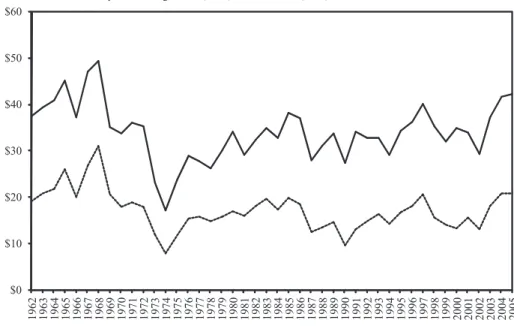
For starters, Figure 2A plots share price breakpoints for low- and high-priced shares. Low-priced stocks are taken to be those with per-share prices below the
30thpercentile of NYSE common stocks. High-priced stocks are those with
per-share prices above the 70th percentile. Average share prices for high-priced
stocks have varied over time from a high near $50 per share in the late 1960s to a low below $20 per share in the early 1970s. Figure 2B plots average share
prices for large-cap and small-cap firms.8Small caps are defined as those with
capitalizations below the 30th percentile of NYSE common stocks and large
caps have capitalizations above the 70th percentile. As noted by prior authors
such as Weld et al. (2009), capitalization and share prices have a very strong cross-sectional relationship, with smaller stocks typically having lower share prices.
These f luctuating share prices are associated with f luctuating valuation ra-tios. Figure 3A plots the average market-to-book ratios of low- and high-price stocks. Market equity is end-of-year stock price times shares outstanding (Com-pustat item 24 times item 25). Book equity is stockholders’ equity (216) (or first available of common equity (60) plus preferred stock par value (130) or book assets (6) minus liabilities (181)) minus preferred stock liquidating value (10) (or first available of redemption value (56) or par value (130)) plus balance sheet deferred taxes and investment tax credit (35) if available and minus
8Like Weld et al. (2009), we exclude Berkshire Hathaway from computations of mean prices.
The price of Berkshire Hathaway stock has been above $10,000 per share since October 1992, and above $100,000 per share since October 2006.
Panel A: Share Price Breakpoints for High-Price (Solid) and Low-Price (Dash) NYSE Stocks $0 $10 $20 $30 $40 $50 $60 1962 1963 1964 1965 1966 1967 1968 1969 1970 1971 1972 1973 1974 1975 1976 1977 1978 1979 1980 1981 1982 1983 1984 1985 1986 1987 1988 1989 1990 1991 1992 1993 1994 1995 1996 1997 1998 1999 2000 2001 2002 2003 2004 2005 Panel B: Average Share Prices for Large (Solid) and Small-Cap (Dash) NYSE Stocks
$0 $10 $20 $30 $40 $50 $60 $70 1962 1963 1964 1965 1966 1967 1968 1969 1970 1971 1972 1973 1974 1975 1976 1977 1978 1979 1980 1981 1982 1983 1984 1985 1986 1987 1988 1989 1990 1991 1992 1993 1994 1995 1996 1997 1998 1999 2000 2001 2002 2003 2004 2005
Figure 2. Share price breakpoints.In Panel A, all NYSE stocks with share codes of 10 or 11
are ranked each year by share price at the end of December. The figure shows the 30thpercentile
and 70thpercentile share price breakpoints. In Panel B, all NYSE stocks with share codes of 10 or
11 are ranked each year by market capitalization at the end of December. The figure shows the
equal-weighted average share price for stocks with market capitalizations below the 30thpercentile
Panel A: Value-Weighted Average Market-to-Book Ratio for High-Price Stocks (Solid) and Low-Price Stocks (Dash) 0.00 0.50 1.00 1.50 2.00 2.50 3.00 3.50 1962 1963 1964 1965 1966 1967 1968 1969 1970 1971 1972 1973 1974 1975 1976 1977 1978 1979 1980 1981 1982 1983 1984 1985 1986 1987 1988 1989 1990 1991 1992 1993 1994 1995 1996 1997 1998 1999 2000 2001 2002 2003 2004 2005
Panel B: Value-Weighted Average Market-to-Book Ratio of Large Stocks (Solid) and Small Stocks (Dash)
0.00 0.50 1.00 1.50 2.00 2.50 3.00 1962 1963 1964 1965 1966 1967 1968 1969 1970 1971 1972 1973 1974 1975 1976 1977 1978 1979 1980 1981 1982 1983 1984 1985 1986 1987 1988 1989 1990 1991 1992 1993 1994 1995 1996 1997 1998 1999 2000 2001 2002 2003 2004 2005
Panel C: The Low-Price Premium (Solid) and Small-Stock Premium (Dash)
-1.00 -0.80 -0.60 -0.40 -0.20 0.00 0.20 1962 1963 1964 1965 1966 1967 1968 1969 1970 1971 1972 1973 1974 1975 1976 1977 1978 1979 1980 1981 1982 1983 1984 1985 1986 1987 1988 1989 1990 1991 1992 1993 1994 1995 1996 1997 1998 1999 2000 2001 2002 2003 2004 2005
Figure 3. The low-price and small-stock premia, and the split announcement premium. The low-price premium is the log difference in the value-weighted average market-to-book ra-tios of low- and high-priced stocks. The small-stock premium is the log difference in the value-weighted average market-to-book ratios of small and large stocks. The market-to-book ratio is the ratio of the market value of the firm to its book value. Market value is equal to market equity at calendar year-end plus book debt. Book equity is defined as stockholders’ equity mi-nus preferred stock plus deferred taxes and investment tax credits and post retirement assets. All NYSE stocks with share codes of 10 or 11 are ranked each year by share price and market capitalization at the end of December. Low (high)-price stocks are stocks with share prices
be-low the 30thpercentile (above the 70thpercentile) by share price. Small (large) stocks are stocks
with market capitalizations below the 30th percentile (above the 70th percentile) by
capitaliza-tion. Panels A and B plot the value-weighted average market-to-book ratios of high- and low-priced stocks and large and small stocks. Panel C plots the low-price and small-stock premia. Panel D plots the split announcement premium, defined as the abnormal return from the day before split announcement through 10 days after the effective date, scaled by the standard deviation of returns.
Panel D: The Split Announcement Premium -0.20 0.00 0.20 0.40 0.60 0.80 1.00 1962 1963 1964 1965 1966 1967 1968 1969 1970 1971 1972 1973 1974 1975 1976 1977 1978 1979 1980 1981 1982 1983 1984 1985 1986 1987 1988 1989 1990 1991 1992 1993 1994 1995 1996 1997 1998 1999 2000 2001 2002 2003 2004 2005 Figure 3. Continued
post-retirement assets (330) if available. The market-to-book ratio is then book assets minus book equity plus market equity all divided by book assets. Simi-larly, Figure 3B plots the average market-to-book ratios of small-cap and large-cap stocks. We show the value-weighted average market-to-book ratios in these
figures but we also compute equal-weighted averages.9 Because of the strong
cross-sectional relationship between size and share price, Figures 3A and 3B look quite similar.
Finally, we translate these valuations into proxies for catering incentives.
Figure 3C displays the low-price premium PCME (“cheap minus expensive”),
which is the log of the average market-to-book ratio of low-priced stocks minus the log of the average market-to-book of high-priced stocks. The figure also
shows the small-stock premium PSMB (“small minus big”), which is the log of
the average market-to-book ratio of small-caps minus the log of the average market-to-book of large-caps. Again, we plot only the value-weighted average measure, but Table II also reports the equal-weighted measure.
Capitalization is positively correlated with the market-to-book ratio, so it is not surprising that on average low-priced and small stocks have sold at a discount in terms of their value-weighted average valuation ratios, with 1983 the lone exception in the value-weighted series. In the equal-weighted average valuation ratios, small stocks displayed a premium valuation ratio from 1979 through 1985 and in both 2003 and 2004. More importantly for this analysis, the equal-weighted premium for high-priced stocks has very similar variation. Historical market commentaries give some color to the peaks and troughs in the low-price and small-stock premia. For example, according to Malkiel (1999), two peaks in Figure 3C, the late-1960s and 1983, were both notable eras for new issues, which tended to be low-priced and of small capitalization. There are also two troughs in which large caps and high-priced stocks were apparently more in favor. One is the early 1970s and ref lects what Siegel (1998) calls the “nifty fifty” bubble. This name refers to 50 large, stable, consistently profitable stocks.
Siegel writes, “All of these stocks had proven growth records. . .and high market
9In computing the equal-weighted averages, we winsorize the market-to-book ratio of individual
Table II
The Low-Price and Small-Stock Premia
The low-price premiumPCMEis the log difference in the average market-to-book ratios of low- and
high-priced stocks. The small-stock premiumPSMBis the log difference in the average
market-to-book ratios of small and large stocks. The market-to-market-to-book ratio is the ratio of the market value of the firm to its book value. Market value is equal to market equity at calendar year-end plus book debt. Book equity is defined as stockholders’ equity minus preferred stock plus deferred taxes and investment tax credits and post-retirement assets. All NYSE stocks with share codes of 10 or 11 are ranked each year by share price and market capitalization at the end of December.
Low-price, that is, cheap stocks (high Low-price, i.e., expensive) are stocks with share prices below the 30th
NYSE percentile (above the 70thpercentile) by share price. Small (large) stocks are stocks with
market capitalizations below the 30thNYSE percentile (above the 70thpercentile) by capitalization.
Each premium is presented with both equal-weighted (EW) and value-weighted (VW) averages. The cumulative abnormal return CAR is the difference between the stock return and the value-weighted market return over the interval that starts the day before split announcement and ends 10 days after the effective date. The split announcement premium is the CAR scaled by the square root of the number of days in the window times the standard deviation of daily returns in the 100 trading days ending 5 days prior to the split announcement date. The average split announcement premium
A is reported in the table. Thet-statistic is from Campbell et al. (2001) and tests the hypothesis
that the average split announcement return is equal to zero.
Split Announcement
Low-Price Premium Small-Stock Premium Premium
PCME PSMB A
Year VW EW VW EW CAR A t-Stat
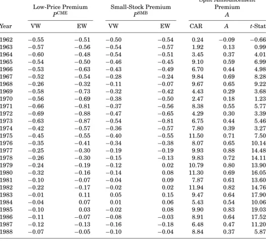
1962 −0.55 −0.51 −0.50 −0.54 0.24 −0.09 −0.66 1963 −0.57 −0.56 −0.54 −0.57 1.92 0.13 0.99 1964 −0.60 −0.48 −0.54 −0.51 3.45 0.37 4.01 1965 −0.54 −0.50 −0.46 −0.45 9.10 0.59 6.99 1966 −0.53 −0.63 −0.43 −0.49 6.70 0.44 4.98 1967 −0.52 −0.54 −0.28 −0.24 9.84 0.69 8.28 1968 −0.26 −0.32 −0.11 −0.07 9.67 0.65 9.22 1969 −0.58 −0.73 −0.32 −0.42 4.43 0.29 3.68 1970 −0.56 −0.69 −0.38 −0.50 2.47 0.18 1.23 1971 −0.66 −0.81 −0.37 −0.56 8.38 0.55 5.77 1972 −0.69 −0.88 −0.47 −0.65 4.29 0.30 3.39 1973 −0.63 −0.87 −0.54 −0.81 6.75 0.44 5.46 1974 −0.42 −0.57 −0.36 −0.57 7.80 0.39 3.27 1975 −0.45 −0.55 −0.40 −0.55 11.50 0.71 7.50 1976 −0.35 −0.41 −0.34 −0.38 8.07 0.65 10.14 1977 −0.25 −0.30 −0.19 −0.19 9.93 0.88 14.48 1978 −0.26 −0.30 −0.15 −0.13 9.83 0.72 14.11 1979 −0.24 −0.19 −0.12 0.02 10.79 0.80 13.90 1980 −0.32 −0.16 −0.14 0.08 11.30 0.69 16.05 1981 −0.10 −0.07 −0.04 0.09 7.87 0.61 13.60 1982 −0.22 −0.17 −0.02 0.02 11.94 0.82 14.76 1983 −0.01 0.11 0.05 0.15 9.47 0.64 17.90 1984 −0.04 0.07 0.01 0.06 5.43 0.54 10.06 1985 −0.10 0.03 −0.02 0.08 9.90 0.83 19.03 1986 −0.11 −0.07 −0.08 −0.03 8.91 0.64 17.52 1987 −0.12 −0.13 −0.16 −0.18 6.48 0.47 11.20 1988 −0.07 −0.05 −0.10 −0.04 8.84 0.37 5.87 (continued)
Table II—Continued
Split Announcement
Low-Price Premium Small-Stock Premium Premium
PCME PSMB A
Year VW EW VW EW CAR A t-Stat
1989 −0.16 −0.15 −0.18 −0.13 7.42 0.57 10.75 1990 −0.31 −0.39 −0.26 −0.25 7.23 0.57 8.11 1991 −0.36 −0.48 −0.21 −0.26 11.23 0.67 11.38 1992 −0.33 −0.29 −0.16 −0.14 11.80 0.72 15.25 1993 −0.23 −0.22 −0.10 −0.07 9.50 0.56 12.74 1994 −0.26 −0.31 −0.17 −0.09 7.31 0.35 6.51 1995 −0.34 −0.44 −0.22 −0.19 10.78 0.65 13.99 1996 −0.36 −0.38 −0.24 −0.19 10.71 0.55 12.66 1997 −0.48 −0.41 −0.31 −0.27 9.03 0.64 14.28 1998 −0.81 −0.77 −0.67 −0.57 5.06 0.23 4.86 1999 −1.00 −0.90 −0.81 −0.64 17.70 0.45 9.20 2000 −0.78 −0.90 −0.74 −0.71 12.08 0.46 8.73 2001 −0.56 −0.48 −0.46 −0.35 8.54 0.51 6.85 2002 −0.52 −0.41 −0.40 −0.29 9.59 0.86 12.16 2003 −0.31 −0.07 −0.23 0.01 7.26 0.45 6.89 2004 −0.24 −0.05 −0.10 0.04 8.31 0.65 10.67 2005 −0.28 −0.08 −0.13 −0.05 6.06 0.54 9.06
capitalization,” and surely high nominal share prices (p. 106). Another trough occurs in the Internet period. This is driven by extraordinary valuations on high-price, large-cap stocks, consistent with the popular impression of a long bull market for the S&P 500 that started in the 1980s. It also ref lects the valuations of many growth stocks that had such high returns that they quickly leapfrogged smaller-cap firms to become high-price, large-cap stocks. Indeed, data from Jay Ritter’s website indicate that the average first-day return among the 1999 IPO cohort was 70%.
Two historical anecdotes seem particularly apropos of the catering hypoth-esis and help illustrate the variation in the low-price and small-stock premia. First, the low-price premium reached its maximum in 1983. Perhaps not coin-cidentally, 1983 also witnessed the proposed offering of startup Muhammad Ali Arcades International in the form of units of one share plus two warrants at
the price of one penny. As Malkiel writes, “. . .when it was discovered that the
champ himself had resisted the temptation to buy any stock in his namesake company, investors began to take a good look at where they were. Most did not like what they saw. The result was a dramatic decline in small company stocks in general” (1999, p. 77–78). As a second interesting anecdote, in 1989, at the tail end of a 15-year period of outperformance of low-price stocks, Fidelity In-vestments launched the Low-Priced Stock Fund. The fund’s mandate was to select stocks trading at $10 or less. Over the next several years—as high-price stocks began to outperform—the definition of “Low-Priced” was raised to below $25 and then to below $35.
In addition to relative valuation ratios, we also use the market reaction to splits as a proxy for catering incentives. When splitting firms are greeted with a positive market reaction (Fama et al. (1969) and subsequent authors find that the average split announcement effect is positive), perhaps the simplest infer-ence is that investors prefer lower prices. More specific evidinfer-ence comes from Greenwood (2009), who shows that Japanese firms split more frequently follow-ing high split announcement effects. He also finds that high split announcement effects are associated with higher split ratios. Both results are consistent with catering. Of course, at least in the United States, positive news about earnings
or dividends news is often announced at the same time as a split.10Another
pos-sibility is that investors mistakenly believe that a stock cut into more shares is worth more; this is consistent with evidence from psychology that people judge the value of something based on the number of units without considering the size or value of those units (Pelham, Sumarta, and Myaskovsky 1994). In using the market reaction to splits as a measure of catering incentives, we are implic-itly assuming that this news content is similar across years or, to the extent it varies over time, that it is not correlated with catering incentives.
Specifically, we compute the return in the window from the day before the CRSP split announcement date through 10 trading days after the effective
date, net of the value-weighted market index.11 To control for differences in
volatility across firms and over time (see Campbell et al. (2001)), we scale each firm’s excess return by the square root of the number of days in the window times the standard deviation of its daily excess returns. We measure volatility in the period from 100 trading days prior to the split announcement through 5 days before the announcement. We label the standardized announcement
effectAand report the average within each year over time. This series is
pre-sented in Table II and in Panel D of Figure 3. The figure shows thatAvaries
considerably over time, from a high of 0.88 in 1977, meaning that the average event return was 0.88 standard deviations above zero, to a low of –0.09 in 1962.
The figure also shows a fairly high degree of correlation betweenAand the
low-price (ρ =45%) and small-cap (ρ =52%) premia. Thus, the valuation benefits
of splitting vary with our premium measures in an intuitive way. We view all of these measures as alternative, but noisy, proxies for catering incentives.
C. Catering Incentives and Splitting Activity
We start by examining whether aggregate measures of split activity, as in equations (5) and (6), are related to measures of catering incentives. Specifically,
10Another possibility is suggested by the psychology literature. Pelham, Sumarta, and
Myaskovsky 1994 define “numerosity” as the heuristic in which people judge the value of some-thing based on the number of units without considering the size or value of those units (Pelham, Sumarta, and Myaskovsky 1994).
11We have experimented with different windows for measuring the announcement premium,
achieving similar results using both shorter and longer windows. We also find that the announce-ment premium is not much affected whether one includes or excludes stock dividends in the
we regress the split percentage and the broader measure of splitting activity on equal- and value-weighted measures of the low-price and small-stock premia and the split announcement premium, controlling for beginning-of-period prices and returns:
st =a+bPtCME−1 +c PtSMB−1 +dAt−1+eptEW−1+ f rtEW+ut, and
mt =a+bPtCME−1 +c PtSMB−1 +dAt−1+eptEW−1+ f rtEW+ut. (8)
We expect the coefficients on the low-price (cheap minus expensive) and
small-stock (small minus big) premia, labeledbandc, as well as the split
an-nouncement effect, labeled d, to have a positive relationship with the split
percentage. In other words, when low-priced and small stocks are trading at a premium relative to high-priced and large stocks, or when splits are associ-ated with larger announcement returns, we expect to see more firms splitting their shares down to lower prices in the hopes of attracting investor demand. The broader measure of splitting activity is decreasing in the propensity to split and the split ratio, so we expect opposite signs. When splits are associated
with high announcement returns, we expect to see firms taking actionsm to
decrease their stock prices. Note in the measureswe include regular splits; it
makes little difference if we include stock dividends. The measuremincludes
all firms and thus is the net effect of splits of any type.
The estimates ofb, c, anddin Table III are broadly consistent with these
predictions. The top panel shows univariate results. All 10 coefficients have the correct sign, and all but two are statistically significant at the 5% level. Standard errors are adjusted for heteroskedasticity and autocorrelation of up to three lags and all of the independent variables are standardized. Thus, in terms of economic significance, a one-standard deviation increase in the value-weighted low-price premium, for example, is associated with a 0.94 percentage point increase in split frequency and a 0.85 percentage point net decrease in prices through price management. Equal-weighting the low-price premium or using the small-stock premium as a measure of catering incentives leads to slightly larger effects. Split announcement effects are associated with split fre-quencies as well as being strongly associated with net decreases in prices.
The bottom panel shows multivariate results that control for the overall equal-weighted average share price from the beginning of the year and the equal-weighted average return over the course of the year. Naturally, split ac-tivity is more common when share prices and returns are generally high. More important for us is that the inclusion of these control variables does not affect
the coefficients on catering proxies, which are similarly strong. In fact, thet
-statistics on catering incentives are typically as high as thet-statistics on the
average price level (unreported), and the inclusion of these variables does not greatly increase goodness of fit relative to univariate regressions that contain only catering incentives. One might have expected the average price level to be the dominant effect on overall split activity, but these results suggest that catering incentives may be as important.
T able III The Low-Price and Small-Stock Premia and Splitting Activity This table presents regressions of the low-price and small-stoc k premia and regressions of measures of splitting activity on the low-price and small -stoc k premia: st = a + bP CME t− 1 + cP SMB t− 1 + dA t − 1 + ep EW t− 1 + fr EW t + ut and mt = a + bP CME t− 1 + cP SMB t− 1 + dA t − 1 + ep EW t− 1 + fr EW t + ut , where s is the number of splits in year t , expressed as a percentage of the number of firms , shown in T able I; m is a summary measure of splitting activity in year t equal to the log of the ratio of the actual a verage stoc k price to the t − 1 stoc k price grown at the stoc k return exc luding dividends; P CME and P SMB are the low-price and small-stoc k premia shown in T able II; and A is the split announcement premium shown in T able II. In the multivariate regressions ,the controls inc lude the log equal-weighted a verage stoc k price p EW in year t − 1 and the log equal-weighted return r exc luding distributions at time t . Eac h regression has 44 observations . All right-hand-side variables ha ve been standardized to unit variance . t -statistics in brac kets use standard errors that are robust to heteroskedasticity and autocorrelation of up to three lags . Split % s Splitting Activity m VW P CME t− 1 0 . 94 1 . 33 − 0 . 85 − 1 . 00 [2 . 32] [2 . 84] [ − 2 . 08] [ − 2 . 42] EW P CME t− 1 1 . 15 − 0 . 86 [3 . 05] [ − 1 . 95] VW P SMB t− 1 1 . 33 1 . 53 − 0 . 93 − 0 . 99 [2 . 99] [3 . 03] [ − 2 . 05] [ − 2 . 19] EW P SMB t− 1 1 . 56 − 0 . 88 [4 . 66] [ − 1 . 75] At− 1 1 . 62 1 . 82 − 0 . 79 − 0 . 82 [3 . 37] [4 . 20] [ − 1 . 55] [ − 1 . 67] pt− 1 1 . 82 1 . 59 1 . 63 − 0 . 74 − 0 . 51 − 0 . 43 [3 . 32] [3 . 28] [3 . 92] [ − 1 . 25] [ − 0 . 86] [ − 0 . 97] rt 1 . 84 1 . 93 0 . 92 − 1 . 69 − 1 . 73 − 1 . 22 [1 . 41] [1 . 57] [0 . 70] [1 . 54] [ − 1 . 70] [ − 1 . 33] Adj. R 2 0 . 08 0 . 14 0 . 19 0 . 27 0 . 29 0 . 18 0 . 27 0 . 38 0 . 12 0 . 12 0 . 14 0 . 13 0 . 10 0 . 13 0 . 14 0 . 08
-0.2 0 0.2 0.4 0.6 0.8 1 1.2 $0 $5 $10 $15 $20 $25 $30 1980 1981 1982 1983 1984 1985 1986 1987 1988 1989 1990 1991 1992 1993 1994 1995 1996 1997 1998 1999 2000 2001 2002 2003 2004 2005 2006 -P CME t-1 or -P SMB t-1
Mean IPO Closing Price
Mean IPO Closing Price
-PCME
-PSMB
Figure 4. The small-stock premium and IPO prices.The average IPO first-day closing price (solid), plotted against the low-price-stock premium (short dash—right axis, inverted) and the
small-stock premium (long dash—right axis, inverted) in yeart−1. The low-price-stock premium
PCMEis the difference between the logs of the value-weighted market-to-book ratios for low- and
high-priced firms. The small-stock premium PSMB is the difference between the log of the value-weighted market-to-book ratios for small and large firms. Data on IPO prices are from Jay Ritter.
D. Catering Incentives and IPO and Post-split Prices
Next we examine IPO and post-split prices, as in equations (4) and (7). These are situations where the firm has explicitly chosen a stock price. Catering pre-dicts that splitters will split to lower prices and new firms will list with lower prices when low-priced firms (or small firms) are more highly valued. In some respects, this is a clearer test. We expect to see more splitting activity simply in response to higher prices and past returns, but we would not necessarily expect to see differences in post-split or IPO prices.
Figure 4 shows the relationship between catering incentives and IPO first-day closing prices. Initial public offerings offer a unique setting to test for cater-ing effects on prices; as the price is highly discretionary, there are strong in-centives to adapt cosmetic aspects of the firm to attract investor demand, and there is no issue of inertia with respect to a particular historical price range. Average IPO closing prices almost tripled from 1984 to 1999 and have fallen more recently. This variation appears to be well explained by proxies for cater-ing incentives, which are inverted and once-lagged in the figure. The figure shows that when the relative valuations of large or high-priced stocks are high, firms go public at higher prices, and vice versa. The correlation between IPO
closing prices and the lagged value-weighted low-price premium is−0.88 and
-0.20 0.00 0.20 0.40 0.60 0.80 1.00 1.20 $0 $10 $20 $30 $40 $50 1963 1964 1965 1966 1967 1968 1969 1970 1971 1972 1973 1974 1975 1976 1977 1978 1979 1980 1981 1982 1983 1984 1985 1986 1987 1988 1989 1990 1991 1992 1993 1994 1995 1996 1997 1998 1999 2000 2001 2002 2003 2004 2005 2006 -P CME t-1 or -P SMB t-1 Mean P o
st-split Price Mean Post-split Price
-PCME
-PSMB
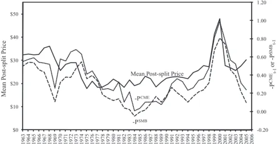
Figure 5. The low-price premium and post-split stock prices.The average post-split price
(solid—left axis) in yeartis plotted against the low-price premium (dash—right axis, inverted)
and small-stock premium (long dash—right axis, inverted) in yeart−1. The average post-split
price is described in Table I and the low-price premium and small-stock premium are described in Table II.
Perhaps the central result of the paper is illustrated in Figure 5, which looks at the larger and longer sample of post-split prices chosen by seasoned firms. The average post-split price is plotted against the low-price and small-stock premia (lagged one period and inverted). The variation in post-split prices is qualitatively similar to the variation in prices chosen by newly public firms. In 2000, for example, the average post-split price was nearly $50—more than double the average price that firms had been splitting to just a few years earlier and roughly double the price that firms would be splitting to a few years later. Measures of catering incentives again help explain this variation. When the low-price premium is relatively high, firms that split do so to lower prices. The correlation between the post-split price and the value-weighted low-price
premium is−0.72. The correlation with the small-stock premium is−0.64. The
2000 spike in post-split prices matches a spike in the relative valuation of small-cap and low-price firms, but there seems to be a correlation in other periods as well.
Somewhat more formally, we regress IPO and post-split log prices on equal-and value-weighted versions of the low-price equal-and small-stock premium equal-and the split announcement premium, controlling for beginning-of-period prices and returns: pIPO t =a+bPtCME−1 +c P SMB t−1 +dAt−1+ep EW t−1+ f r EW t +ut, and pt =a+bPtCME−1 +c PtSMB−1 +dAt−1+epEWt−1+ f rtEW+ut. (9)
We expectb,c, anddon actively chosen prices to be negative. In other words, when low-priced and small stocks are trading at a premium, or when splits to lower prices are associated with a larger announcement effect, we expect to see
firms choosing lower prices.12
The estimates in Table IV are consistent with predictions. The top panel shows univariate results, and the bottom panel controls for past prices and contemporaneous returns. All coefficients have the expected sign and almost all are statistically significant at the 5% level. In terms of economic significance, a one-standard deviation increase in the low-price premium is associated with a 19 percentage point decrease in IPO prices and a 17 percentage point decrease in post-split prices. Results for the small-stock premium are similarly strong. These effects are only slightly affected by the inclusion of average prices and recent returns as control variables, and the inclusion of such controls increases the statistical and economic significance of the split announcement premium. In the IPO price regressions, we obtain similar results irrespective of whether the dependent variable is the IPO offer price, the first-day closing price, or the midpoint of the filing range (see the Internet Appendix for a complete
tabula-tion).13
E. Robustness Checks
We test several aspects of the robustness of the link between catering incen-tives and post-split prices. The details of these calculations are available in the
Internet Appendix.14
We start by examining whether the results come predominantly from one part of the sample. Splitting the sample into halves indicates that this is not
the case, as the coefficients and t-statistic are nearly identical. Nor are the
results driven by the Internet peak, which appears prominently in some of our figures, as shown by the fact that strong results obtain even upon excluding the 1998 to 2001 or 1998 to 2005 periods.
A second concern is that both the premia and the average post-split price may share a common time trend, leading to a spurious correlation. But controlling for a time trend only strengthens the results. We also go a step further and run equation (9) in differences, removing the time trend from both series. The dependent variable is the change in the log post-split price, and the independent variable is the lagged change in the low-price (or small cap) premium. Again,
results are similar.15
12We use log prices as dependent variables here, but we obtain similar results using dollar
prices.
13The explanatory power of the regressions drops if we use the midpoint range. For example,
the adjustedR-squared from 0.78 in the first column in Table IV to 0.31 if the dependent variable
is the log of the average midpoint price.
14An Internet Appendix to this paper is available at http://www.afajof.org/supplements.asp.
15Related to the difference specification, we estimate GLS specifications based on a variant of
the Cochrane–Orcutt procedure, which assumes that regression residuals are AR(1). Again, the results are similar and significant. In other untabulated results, we find that the level of the log post-split price is significantly related to past changes in the low-price (or small-cap) premium.
T able IV The Low-Price and Small-Stock Premia and IPO and P ost-split Stock Prices This table presents the results of regressions of price levels on the low-price and small-stoc k premia: p IPO t = a + bP CME t− 1 + cP SMB t− 1 + dA t − 1 + ep EW t− 1 + fr EW t + ut and pt = a + bP CME t− 1 + cP SMB t− 1 + dA t − 1 + ep EW t− 1 + fr EW t + ut , where p IPO is the log of the a verage IPO price in year t , p is the log of the a verage post-split stoc k price in year t , and P CME and P SMB are the low-price and small-stoc k premia shown in T able II; A is the split announcement premium shown in T able II. In the multivariate regressions , the controls inc lude the log equal-weighted a verage stoc k price p EW in year t − 1 and the log equal-weighted return r exc luding distributions at time t . All right-hand-side variables ha ve been standardized to unit variance . Eac h p IPO regression has 27 observations , and eac h p regression has 44 observations . t -statistics in brac kets use standard errors that are robust to heteroskedasticity and autocorrelation of up to three lags . IPO Price pIPO P ost-split Price p VW P CME t− 1 − 0 . 19 − 0 . 17 − 0 . 17 − 0 . 12 [ − 10 . 24] [ − 8 . 63] [ − 6 . 47] [ − 4 . 00] EW P CME t− 1 − 0 . 18 − 0 . 12 [ − 4 . 93] [ − 2 . 81] VW P SMB t− 1 − 0 . 18 − 0 . 16 − 0 . 15 − 0 . 12 [ − 6 . 96] [ − 8 . 00] [ − 5 . 02] [ − 4 . 52] EW P SMB t− 1 − 0 . 20 − 0 . 11 [ − 4 . 55] [ − 2 . 11] At− 1 − 0 . 12 − 0 . 14 − 0 . 10 − 0 . 07 [ − 1 . 38] [ − 2 . 21] [ − 3 . 51] [ − 2 . 62] pt − 1 0 . 14 0 . 23 0 . 36 0 . 21 0 . 24 0 . 26 [2 . 92] [8 . 19] [2 . 60] [7 . 22] [8 . 34] [10 . 85] rt 0 . 23 0 . 31 0 . 50 0 . 09 0 . 08 0 . 13 [2 . 13] [3 . 10] [3 . 67] [1 . 67] [1 . 85] [1 . 67] Adj. R 2 0 . 78 0 . 57 0 . 69 0 . 52 0 . 12 0 . 81 0 . 82 0 . 44 0 . 51 0 . 26 0 . 39 0 . 19 0 . 16 0 . 79 0 . 80 0 . 62
We also use past relative returns of cheap and expensive stocks and small and large stocks in place of valuation premia. We compound these differences over
the 3 years prior to yeartand use the gap in returns to predict the average
post-split price in yeart. As expected, the basic results are qualitatively unchanged.
In the IPO specifications, we replace first-day closing prices with offering prices. Although Loughran and Ritter (2002) show that the closing price is predictable, the offering price may be a better gauge of the intended share price. In any event, the results are not sensitive to this distinction, though the coefficient increases as a result of the lower variance of offering prices.
Another conceivable issue with the results in Table IV involves a composi-tion effect. Suppose that small firms always split to low prices and large firms always split to higher prices. Then, when small-cap or low-price premia are high, we would expect more small firms to be potential splitters. Since small firms split to lower prices, the average post-split price will be lower, potentially producing the effect in Table IV. An easy test of this alternative explanation is to separate small from large firms. We define small firms as those with market
capitalization less than the 30thNYSE percentile and large firms as those with
market cap greater than the 70th percentile. Our results are driven by large
firms, suggesting that large firms “act small” when catering incentives point in that direction, rather than the composition effect suggested above. Perhaps smaller listed firms have less scope to alter investor perceptions, especially if their prices are already low (reverse splits are rare as shown in Table I). At the same time, the results for IPO prices involve smaller and younger firms, and so catering incentives seem important at various stages of the firm life cycle.
In another check, we estimate low-price and small-stock premia based solely on profitable firms, to account for the fact that some low-price and small stocks are distressed. This has little effect. Finally, we split the low-price and small-stock premia into their components. This addresses a class of alternative expla-nations in which our catering incentives measures are correlated with overall valuation levels. For example, high overall valuation levels may proxy for low expected returns, so perhaps firms choose not to split to low prices because they expect their price to fall on its own. A simple test is to see whether the effect is coming from both or just one part of our relative valuation measures. The results suggest that post-split prices are significantly positively related to the valuations of high-priced (or large) stocks as well as significantly negatively related to the valuations of low-priced (or small) stocks.
A class of explanations that is popular in the splits literature involves sig-naling. It is hard to rule out signaling as an explanation for any particular split or pattern of a firm’s decisions. For example, Applied Materials may have split to lower prices because of increased confidence that its current valuation would rise. However, signaling is unlikely to explain our large-sample results. We find a pattern between publicly available data (the relative valuation of low- and high-priced firms) and the propensity to split. While this could ref lect time-series variation in asymmetric information, it would more naturally pre-dict that the need to signal was greater, not lesser, when low-priced and small stocks (opaque firms) were trading at a discount.
III. Firm-Level Tests
As another robustness test we can use firm-level data. This allows us to more fully control for composition effects that could affect average post-split prices and split activity but that do not involve catering, as well as to correct for ef-fects related to variation over time in the cross-sectional dispersion in prices or other relevant characteristics. The specific approach is to add time-series mea-sures of catering incentives to pooled firm-level regressions corresponding to equations (4) through (7).
A. Data
We gather firm- and industry-level determinants of splits and post-split share prices at an annual frequency. We take beginning-of-year nominal share prices and construct annual stock returns using CRSP data. We measure firm size as the NYSE capitalization decile as of the end of the previous calendar year. We control for industry average prices using Fama and French (1997) industry classifications, updated using data from Ken French’s website. In some cases we also control for idiosyncratic, firm-specific preferences for a specific price range by using the price to which the firm previously split (regardless of whether the split was a regular split, stock dividend, or reverse split). Inclusion of this last control limits the sample to firms that have split previously.
B. Catering Incentives and Firm-Level Splitting Activity
In Table V, we estimate the firm-level analog to our time-series regressions
in Table III. An indicator variable equal to one when firmisplits or pays a stock
dividend in quartertreplaces the aggregate split percentage, and the firm-level
measure of the net impact of splitting activitymreplaces the equal-weighted
average across firms. We regress these dependent variables (using probit for the dichotomous split decision) on the value-weighted low-price premium,
con-trolling for beginning-of-period log pricesp, contemporaneous log returnsr, the
NYSE size decileNYSED, lagged total return volatilityσ, the industry average
pricepIndustry, and the price at last splitpLastSplit. We cluster the residualsuby
year to match the variation in the low-price premium:16
Pr(si,t=1)=a+bPtCME−1 +epi,t−1+ f ri,t+ gNYSEDi,t +hσi,t−1+ j piIndustry,t−1 +kpiLastSplit,t−1 +ui,t, and
mi,t= pi,t−pi,t−1−ri,t=a+bPtCME−1 +epi,t−1+ f ri,t
+gNYSEDi,t+hσi,t−1+ j pIndustryi,t−1 +kpLastSpliti,t−1 +ui,t. (10)
As before, we expect the coefficient on the low-price premium b to have a
positive sign in the first equation and a negative sign in the second. We expect
16We also estimatet-statistics following Thompson (2006), who describes a technique for
obtain-ing standard errors when residuals are clustered both by firm and in time. Although this adjustment
appears to matter for many of the control variables, it does not much affect the significance ofb,