Is East Asia less open than North America and the European Economic Community? No

POLICY RESEARCH WORKING

PAPER

X

Is

East Asia Less Open than

North America and the

European Economic

Community? No

An'ind Pangaraiya

The World

Bank

OEonomics

Deparmnt

IT>enadonal

Trade Division

Public Disclosure Authorized

Public Disclosure Authorized

Public Disclosure Authorized

POLICY RESEARCH WORIONG PAPER 1370

Summary findings

To shed light on regional integration schemes in North equations. In some cases, this difference is qualitative. America and Europe (and on the alleged trading bloc in Not surprisingly, in virtually all cases the cross-country

East Asia), Dhar and Panagariya explore the nature of equation masks large differences among countries. The bilateral trade relationships. coefficient associated wit!1 distance, for example, varies

Using the gravity model, they conduct an econometric between -4.4 and -O.4 across the authors' equations. In analysis of trade flows between major trading countries, almost every case the coefficienc is statistically significant They estimate bilateral trade flow equations using a data at a confidence level of 95 percent or more.

set for 45 counrries over 12 years and then use those * If there is an incra-regional bias in trade, it is more equations to study the contribution of trading blocs to in North America and among the founding members of intra-regional trade. the European Union than in East Asia. Canada, the

Past investigators have estimated the gravity equation United States, and all countries of the EEC show an using data for total trade, pooling data across countries. intra-regional bias in both exports and imports. In East Dhar and Panagariya estimate separate equations for the Asia, on the other hand, exports in six out of nine exports and imports of 22 countries (nine in East Asia, countrics have a statistically significant bias away from six in Europe, three in North America, two in South intra-regional markets.

America, and one in Oceania). * There is little support for the hypothesis that East Using 27 countries outside of North America, East Asian markets are closed to trade with outside countries. Asia, and the founding members of the European Union * Contrary to conventional wisdom, controlling for

(EEC) as the control countries, Dhar and Panagariya test other variables, many countrics export less to North for each region's openness to trade with outside America than to countries outside the three regions. countries. Similarly, countries outside the EEC export more to the

They conclude that: EEC than to countries in the control group. Results based on individual-country equations differ

greatly from those obtained from pooled, cross-country

This paper - a product of the International Trade Division, Internatonal Economics Department - is part of a study

funded by the Bank's Research Support Budget under the research project 'Understanding Bilateral Flows: An Application to EastAsia" (RPO 677-86). Copies of this paer are available free from the World Bank, 1518 H StreetNW, Washington, DC 20433. Please contact Jennifer Ngaine, room R2-054, extension 37959 (39 pages). October 1994.

The Polsiy Research t orkbg Paper SLeot dismiates the fdings of worvk M prgess to encowge the exhange of ideas abou develpment is An objcfive of the series isto get thefidngs otquk, cevn if Ohepretadtionsare less than fuiy pdished The paprs cay the gmes of tfheauws and osdd besadadciedacordigly. The fldgs _ , and condcrons are the

Is East Asia Less Open than North America

and the European Economic Community?

No

Sumana Dhau

Arvind Panagariya*

*

Dhar is with the In

nal Trade Division,

World Bank,

and the Department

of

Econom-ics, University

of North Carolina,

Chapel

Hill P3nagarya

is with the Center for Intemaional

Econom-ics, Department

of Economics,

Uniesity of Maryland,

College

Park. The authors

tiank Paul

Table of Contents

1. Introduction 1

2. Rationale and Diagnostic Tests 5

3. Estimation 11

3.1 The Basic Equation 12

3.2 Introducing Regional Dummies: Is East Asia different? 15

3.3 Introducing the "Other Region" Effects 19

4. Conclusion 22

References 25

1. Introduction

Paradoxically, both the revival of regional integration around the world and disintegration of the CMEA and the Soviet Union have led to a renewal of interest in the gravity equation. On the one hand, Krugman (6Y91), Frankel (1993) and Saxonhowse (1993) have applied the model to study regional biases in international trade while, on the other, Collins and Rodrik (1991), Havrylyshyn and Pritchett (1991), and Wang and Winters (1991) have used it to predict post-reform trade flows of the countries in Eastern Europe and ex-Soviet Union.

Traditional theories of international trade focus almost exclusively on the determinants of a country's exports and imports and do not address the issue of the direction of trade. As such, theories which provide guidance on the determinants of direction of trade are virtually nonexistent.1 Yet, in the context of regional integration schemes such as the European Economic Community (EEC), European Free Trade Area (EFTA), North American Free Trade Agreement (NAFTA) and the alleged East Asian trading bloc, an understanding of bilateral trade relationships is critical-' Not surprisingly, because it forms the basis of econometric analysis of bilateral trade flows, interest in the gravity equation has risen with the interest in regionalism. The equation has yielded consistently better fits than any other empirical relationship in

'Perhaps the only paper which focuses on this question is the relatively recent paper by Markusen (1986). Markusen constructs a model with three regions - two in the North and one in the South - and neatly combines scale economies, product differentiation, non-homothetic preferences and factor-endowment differences to generate a realistic pattern of trade. For plausible configurations of factor-endowment differences, he shows that the regions in the North must trade in differentiated products with each other and each of them must also export these products to the South in return for homogeneous products. The model also predicts a larger volume of trade between the two capital-abundant Northern regions than between each of them and the South.

international trade literature.3

The gravity model was pioneered independently by Tinbergen (1962) and Poyhonen (1963) and extended by Linneman (1966). The first two authors postulated that bilateral trade flows are related positively to the GDPs of the trading countries and negatively to the distance between them; the last included populations of the two countries as explanatory variables in the model. Though the broad objective of the original authors was to identify the determinants of bilateral trade flows, subsequent investigators have gone on to employ the model for at least three additional purposes. First, the equation has been employed to test whether preferential trading arrangements including free trade areas (FTAs) and customs unions (CUs) have a statistically significant effect on bilateral trade flows. Second, the equation has been employed to test the Linder hypothesis that trade in manufactres is more intense among rich countries with similar per-capita incomes. Finally, the equation has been used to predict equilibrium trade flows of formerly socialist countries in the post-reform era.

Aitken (1973) was the first one to test for the effects of regional arrangements on trade flows. Introducing dumnmy variables for trading partners belonging to the same regional grouping (EEC or EFTA), he found statistically significant effects of these arrangements. Later, Thursby and Thursby (1987) and Bergstrand (1985, 1989) also included dummy variables for the EEC and EFTA in their equations but obtained mixed results. More recently, as noted above, Frankel (1992) and Saxonhouse (1993) have used the gravity equation to test whether there is a de facto trading bloc in East Asia. The former uses Aitken's equation in a slightly modified form and estimates it for total bilateral trade flows, while the latter introduces factor

endowments into the equation and estimates it for several 3-digit SITC commodity groups. Both reject the hypothesis of a trading bloc in East Asia.

The Linder hypothesis has been the main focus of the contributions by, inter alia, Thursby an Thursby (1987), Balassa and Bauwens (1988), and Hanink (1990). All these studies fmd strong support for the hypothesis that similar rich countries trade more intensively with each other in manufactures than dissimilar ones. The use of the gravity equation for predicting trade flows is of a more recent origin. Demise of the CMEA and the Soviet Union and a move towards more liberal and outward oriented policies has meant that trade flows of these economies will be drastically reoriented. Collins and Rodrik (1991), Havrylyshyn and Pritchett (1991) and Wang and Winters (1991) have all applied gravity equations estimated for market economies to predict trade flows of the countries in Eastern Europe and the ex-Soviet Union in the post-reform equilibrium.

In this paper, we subject the gravity equation to a far more careful and detailed econometric analysis than has been done to-date. We then re-examine the issues of regional trading blocs using the esfimated equations.' In a companion paper, Dhar and Panagariya

(1994), we also examine the issue of prediction of trade flows using the gravity model.5

Purely in terms of the quality of estimation, we contribute to the literature in three important ways. First, we work with a much larger data set than done by anyone so far. Second, with the sole exception of Thursby and Thursby (1987), authors have pooled the data

4IFor a discussion of various policy issues relating to the regional option for East Asia, see

Panagariya (1993).

s Srinivasan and Canonero (1993) simulate the effects of preferential trading in the context of South Asian countries.

for different countries and gone on to fit the same equation to trade flows of all countries in the sample.6 _{Our statistical tests lead to an unequivocal rejection of the hypothesis that the}

coefficients across countries are identical. Therefore, we estimate the equation separately for each country and present 22 such cases in this paper. Finally, most investigators (e.g., Aitken, Frankel, and Bergstrand) have estimated the equation using total trade rather than exports and imports separately. We test the hypothesis of equality of coefficients for exports and imports for all countries and overwhelmingly reject it. We then estimate separate equations for exports and imports.

These methodological changes lead to a richer set of results than obtained so far. The conclusions drawn from individual country equations are very different from those obtained from traditional pooled, country equations. In virtually all cases, not surprisingly, the cross-country equation masks large differences across countries, even after inclusion of summary measures for variation in policy and size. For example, the coefficient associated with distance varies between -4.4 and -0.44 across equations.

Intra-regional bias in trade is to be found more in North America and the EEC than East Asia. Canada, the U.S.A. and all countries in the EEC show intra-regional bias in exports as well as imports. In East Asia, exports of 6 out of 9 countries have a statistically significant bias

away firom intra-regional markets. We also compare the openness of each of the three regions

with a control group of 27 countries outside North America, EEC and East Asia. Our results

6 Thursby and Thursby include several short-mn variables such as the exchange-rate

variability and prices in the equations. This mixing-up of short run and long run variables inevitably influences their results. In this paper, we follow closely the pure gravity equation as, for example, in Aitken (1973) and Frankel (1992) and include only the long-run variables.

do not support the hypothesis that East Asian markets are closed to outside countries. Cetris

paribus, for countries outside the EEC, exports to the EEC are larger than to countries in the

control group. Most surprisingly and contrary to the conventional wisdom, controlling for other variables, exports to North America are less than to countries outside the three regions for all EEC countries and Australia!

The paper is organized as follows. In Section 2, we discuss the basic gravity equation and its rationale and report diagnostic tests performed to arrive at particular form(s) in which we estimate it. In Section 3, we estimate the equation for a group of 22 countries and discuss its implications. In Section 4, we make concluding remarks.

2. Rationale and Diagnostic Tests

Gravitational force between two bodies is directly proportional to the mass of those bodies and inversely proportional to the distance between them. By analogy, the gravity equation postulates that bilateral trade flows are directly proportional to the mass of the two nations (represented by their GDPsj and inversely proportional to the disance between them. This basic relationship is often augmented by inclusion of other variables such as per-capita GiDPs of the two countries, a durvay variable for a common border and other dumy variables to represent memberships in different regional arrangements.' Because a key issue we wish to address concerns the presence of regional trading blocs in Europe, North America, and East

7 _{Rationale for the inclusion of price and exchange rate variables by Thursby and Thursby}

(1987) and Bergstrand (1985, 1989) is derived from essentially partial equilibrium models. Bergstrand lays out a general equilibrium model but then chooses not to solve for equilibrium prices. As illustrated in Anderson (1979) and Markusen (1986), once we solve for prices, only income or endowments variables should appear in the equation. This is particularly true if we are interested in the determinant of long-run trade flows.

Asia, we can represent this relationship by

InTJ'

P

Pln(DISTANCFI4

p

n(GDP?

In(FCGDP

(1)

+ P(NAj) + 39A) +

i 1..&, j l... n; i o j; n, s n,.

where superscript i denotes the reporter country, j the partner country, na the total number of reporter countries in the sample and nj the total number of partner countries. Traditionally, this equation is estimated in natural logarithms of the variables. TJ stands for either the value of exports from country i to country j or the value of imports into country i from country j or the sum of the two (i.e., total value of trade between i and

j).

DISTANCE} denotes the distance between countries i and j and GD? and PCGDPi the total and per-capita gross domestic product of country i, respectively. BORDIER and the last three variables are dummy variables. The former equals 1 if i and j have a common border but 0 otherwise. EC6J takes a value of 1 if i and j are both in the EEC but 0 otherwise. NAj and EA,J have a similar interpretation where the former stands for North America and the latter for East Asia.8

Equation (1) does not have a strong theoretical foundation and the reasoning behind the

8 Unless otherwise noted, EEC (EC6) includes the original six members, NA comprises Canada, USA and Mexico, and EA is defined to cover the ten countries in East Asia listed in Appendix 1.

explanatory variables is largely intuitive.9 Distance is expected to have a negative coefficient because transport costs rise and access to information may decline as distance rises. Controlling for distance, adjacency (BORDER) is expected to contribute positively to trade because of possibilities of border trade and cultural and linguistic ties which may not be picked up by distance. This effect is not entirely unambiguous, however; if there is hostility between neighboring nations, the effect may be the opposite. Controlling for per-capita GDP, GDPs are thought to have a positive effect on the absolute level of trade and this can be shown with the help of a multi-country, multi-good Ricardian model (Anderson 1979). It is possible (though not plausible), however, for the reporter country's GDP to have a negative effect on the value of its trade. For example, in the Heckscher-Ohlin model, if all factors expand proportionately in the reporter country, the latter's per-capita GDP remains unaffected while the GDP rises. If the e.asticity of foreign demand for the country's exports is sufficiently low, even though the quantities of exports and imports rise, their value may decline.10 Per-capita incomes are generally hypothesized to have a positive effect on trade because, controlling for the GDP, the higher the per-capita income the greater the demand for differentiated products and the greater the degree of specialization in production. Here again, the argument is not watertight. According to the Linder hypothesis, trade expands with a reduction in differences in per-capita incomes. This suggests opposite signs for per-capita incomes of the two countries." The last

9 A post rationalizations of the gravity equation include Anderson (1979) and Bergstrand (1985, 1989).

10 For more on this, see Thrsby and Thursby (1987) and Bergstrand (1985, 1989). 1 Thursby and Thursby (1987) postulate it by the absolute difference in per-capita incomes of reporter and partner counties.

three dummy variables test for possible regional bias and are expected to have posidtve signs. Frankel (1993) is the main author who uses the tradftional gravity equation to address the issue of an East Asian trading bloc. The equation he employs is slightly different from ours, To wit, he estimates the equation in the form

In?)

acIaln(DISTANCEJB)

(1')

+ a4U(OCGDP.PC3DPj) +

as(C6b

In effect, Frankel restricts equation (1) such that coefficients associated with the reporter- and partner-country GDPs and those associated with the two per-capita GDPs are identical. Since theory does not give a clear guidance on the signs of the reporter-country GDP and per-capita GDP and our tests do not support the hypothesis of equality of coefficients between the two GDPs and per-capita GDPs, we have chosen to report the results using the more flexible form in (1).

Our data set includes annual data on 45 countries listed in Appendix 1 for years 1980-92. The sample includes aIl the OECD countries, and all the countries with significant amount of trade in East Asia, South Asia, and Latin America. We excluded the countries in Africa primarily because the quality of data in that region is significantly poorer than elsewhere and because the distance variable in that region does not capture the same factors as elsewhere due to poor accessibility in general. We also excluded the countries in Eastern Europe and the Soviet Union. Because the observed data for 1992 was incomplete at the time of writing, we used it only to compare against the predictions from our estimated equations for that year (Dhar and Panagariya, 1994).

We subject the data to tbree diagnostic

tests. First, we tested for heteroskedasticity. We

rejected the hypothesis

of no heteroskedasticity

with the probability of 99.99% in all our tests.

Therefore, we applied the Huber-White

correction to all our coefficients

and test statistics.

Second, we formally tested the hypothesis

of equality of coefficients across countries.

Equation (1) is traditionally estimated by pooling the data for all reporter countries for one or

more years. This amounts to the restriction that exports of, say, Venezuela, follow the same

relationship

as exports of U.S.A. Because this seemed unlikely to us, we chose to test formally

the hypothesis that the coefficients in equation (1) are identical across countries.'

Because the test is slightly tricky, it is useful to spell it out explicitly. The country

equation equivalent to (1) takes the fcrm

InST

P

(DSTANC4)

P2(BORDER!

+

PhIn(GDPjt)

p(EC6j

(2)

+ K A) + PI4EA + u

j = 1,... t = 1980,...1991; i *j.

The coefficients, distinguished

by superscript i, are now country specific. The time subscript

is denoted by

In a country equation, there being only one reporter, the cross-country

1 At the minimum, one must control for country-specific

fixed effects. If this is not done,

the regional dummies in (1) and (1') are likely to pick up country-specific

effects rather than the

pure "regional" effect.

13

We can fix t to any particular year and still estimte (2) using 44 observations

for a given

source of variation is absent.'4 _{Because the correlation coefficient between the reporter GDP}

and per-capita income for most of the 22 countries for which we estimated the equations exceeded 0.9, we have dropped PCGDPi as an explanatory variable in (2).

Returning to the test for pooling, recall that as defined, regional dummies take a value of 1 if both the reporter and partner belong to the same region and 0 otierwise. Therefore, for a given estimated equation, if the reporter (country i) does not belong to any of the three regions, the last three variables are equal to zero. If i belongs to one of the regions, two of the three dummy variables sfill take a value of zero.

These observations imply that in testing the hypothesis of equality of coefficients across reporting countries, we must include the coefficient associated with a regional dummy only when comparing two countries in the same region. In all other cases, the regional duy should be excluded because either the dummy does not enter the equation (as in the case of counties not belonging to any region) or the regional dummies in the two equations are different (as when they belong to different regions).

To limit the number of cases, we chose to apply the test to exports from a total of 22 countries to 44 partner countries.15 The reporter countries include 9 countries from East Asia (minus China). 3 from North America, 5 from the EEC (Belgium and Luxembourg appear as one in the data) and 5 outside these regions.1 6 _{Even then, limiting the test to exports alone,}

1 4_{1In pooled cross-country data there is sufficient variation in population across counties}

to rule out multicollinearity between the GDP and per-capita GDP. I Countries listed in Appendix 1 are the 45 partners in trade.

16 Focus on the issue of regional bias in trade made us include the major players in the three

regions. If regional effects prevail, they must exist in the original members of the EEC and the major countries in Fast Asia and North America. Unfortunately, China was dropped from the

we have 231 pairs of countries to compare. We rejected the null hypothesis of the equality of coefficients across countries in every one of these cases with 99.99% probability. Indeed, in the majority of the cases, the much stronger hypothesis of equality of individual coefficients was rejected with a 90% or higher probability.

Our final diagnostic test was with respect to the equality of coefficients across exports and imports of a given country. We carried out this test for the 22 countries mentioned earlier and rejected the null hypothesis that coefficients in the export and import equations are equal with a probability of 99.99% in each case.

3. Estination

Based on our diagnostic tests, we estimate separate export and import equations, without PCGDP, for each of the 22 countries using the Huber-White correction. For purposes of comparison, we also estimate the gravity equation by pooling data from these same 22 reporter countries. The latter is presented at the bottom of Tables 1, 2 and 3. For brevity, we discuss only the equations for exports in detil. Import equations are discussed only when the results are different from those of export equations. Both export and import equations are presented at the end of the paper.

3.1 The Bsasic Equation

We begin by estimating (2) in the simplest form, dropping all regional dummy variables (Table 1A). Measured by both the adjusted R2 _{and root mean square error (MSE), on the}

average, country-specific equations give better fits than the pooled equation. For exports, in 16

list due to unavailability of data over the entire sample period. For comparison purposes, we also included two countries in Latin America, one in South Asia, one in Europe and Australia in our sample.

out of 22 cases, the country-specific

equation does better on the basis of both the adjusted ii

or root MSE. In two additional cases, it does better on the basis of one of the two criteria.

Countries for which the adjusted R

_{is lower and/or root MSE is higher than in the pooled}

equation are Argentina, Mexico, Indonesia, Korea, Taiwan (China) and Singapore. Fits for

fast-growing countries of East Asia, particularly Korea and Singapore, and for Argentina and Mexico

are consistently poor. A large proportion of the variation in exports and imports of these

countries is not explained by the limited number of explanatory variables used in. our

regressions. Remarkably, fits for India are very good suggesting perhaps that though the

controls may have influenced the level of trade, the direction of trade was detemiined by

conventional

variables.

Perhaps the most stiking point is that for countries in the EEC and Japan, the adjusted

R

_{lies between 0.83 and 0.91. Thus, for these countries, both imports and exports are largely}

explained by the smal number of variables included in our equation. Room for any regional

variables to add to the explanatory power is limited. One is almost tempted to reject the

hypothesis

of major regional effects in these countries and terminate investigation

at this point.

But this is perhaps hasty and unscientific.

Turning to individual coefficients,

DISTANCE has a negative and statistically

significant

coefficient (at 99% level) in 37 out of 44 cases.'

_{This is not surprising in view of what is}

already known from gravity equations estimated using pooled data. What is surprising is that,

'

_{Canada and U.S.A. are the only countries where the coefficient}

_{has a positive sign in both}

export and import equations. But later, after we control for all regional effects (Tables 3A), the

coefficient of distance in all cases except Korea becomes positive and statistically significant.

The fit for Korea has been consistently

poor with adjusted R

lying between 0.28 and 0.5.

unlike the impression conveyed in the literature on the basis of pooled gravity equation (e.g., Anderson, 1979), the value of the coefficient varies considerably across individual countries and differs from -1 (in most cases, even statistically significantly). For exports, the coefficient ranges from -0.5 for Great Britain to -3.5 for Indonesia. In the pooled equations shown at the bottom of Table 1A, the coefficient does turn out to be close to -1, with extremely high t-ratios. Next, consider the coefficient of BORDER. A common conclusion from the pooled gravity equation is that, controlling for distance, the presence of a common border contributes positively to trade. This is borne out by both of our pooled equations. The coefficient is 0.35 for the export equation with t-ratios in excess of 3. But, as in the case of DISTANCE, the common coefficient for all countries in the pooled equation hides substantial cross-country differences.' Indeed, when estimated at the level of the country, in some cases, even the sign of the coefficient switches- For example, in the case of India, as one will expect on the basis of hostility between her and China and Pakistan, the coefficient is negative in both the export and import equation. For reasons that are not entirely clear, a common border also contributes negatively to the exports of Mexico, Thailand, Indonesia and Malaysia. For the latter two countries, imports are also negatively related to common border. When positive, the actual size of the coefficient varies considerably across countries. Tue coefficient is much smaller for the EEC countries and has high t-ratios. This may be because trade with countries that have a common border but do not belong to the EEC is not so intense.

GDPj or the partner country GDP has a positive impact (with very strong t-ratios) on

IS Australia, Japan, Korea, Taiwan and ffie Philippines do not have a common border with

both bilateral exports and imports of all countries considered. In the pooled equation for both exports and imports, the coefficient has a value around 0.85. In country-specific equations the coefficient varies between 1.4 and 0.5. Except for exports of Argentina and Mexico, PCGDPJ, the per capita GDP of the partner country also has a positive and, in most cases, a statistically significant effect on trade. This is consistent with the usual results from pooled regressions.

As noted before, GDP`, the reporter-country GDP, switches signs quite frequently across countries when PCGD1", the reporter per-capita GDP, is also included in the equation. As our results show, this problem is alleviated considerably once we drop per-capita GDP from the equation. Only for Canada's exports does this variable have a negative and statistically significant coefficient. In more than half of the cases -26 out of 44 - the sign is positive and highly significant. This sign is far more stable than in Thursby and Thursby (1987).

3.2 hriJreducing Regional Dummies: Is East Asia different?

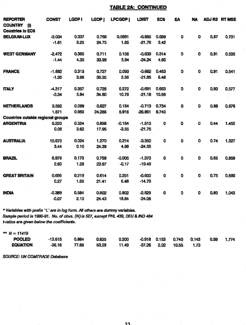
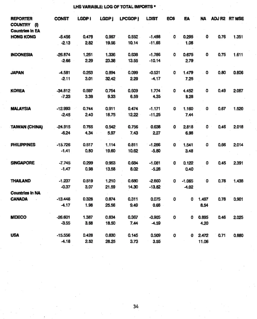
In Table 2A, we introduce the first set of dummies aimed at capuring regional effects (equation 2). The question under investigation is whether East Asia exhibits significantly different intra-regional characteristics from other countries trading within their own region. EC6, EA and NA take the value of when both the reporter and partner in a bilateral trade relation belong to the EEC, East Asia and North America, respectively. If one or both partners do not belong to these regions, the value is 0. For Argentina, Australia, Brazil, Great Britain and India, estimated equations remain the same as in Table IA. For other countries, we have one extra variable.

A critical issue in introducing the regional dummy is possible multicollinearity between it and BORDER. We checked the correlation between these two variables for each individual

country and the group of 22 as a whole. For the cross-section of 22 countries, correlations between BORDER on the one hand and EC6, EA and NA on the other are 0.34, 0.06 and 0.23,

respectively. For countries in North America, the correlation is 0.7 or more. In the case of the United States, the two variables become identical. In the EEC, with the exception of Italy, the correlation lies between 0.57 and 0.86. At the country level, the correlation is low only in East Asia. There the correlation coefficient is 0.3 or lower (except for Malaysia where it is 0.53). This implies that we cannot include both the regional dummy and BORDER as explanatory variables, except in the cross-section equations, Italy and the countries in East Asia region.

We estimated (2) both with and without the BORDER dummy. We found that differences in results even for countries with low correlation between this variable and the relevant regional dummy, in terms of the adjusted

RI

equations for Argentina and Brazil show a noticeable fall in explanatory power when BORDER is dropped from the equation. Broadly, the importance of a common border diminishes once we control for the common region.

For ease of comparison, we choose to present the results when BORDER is dropped as an explanatory variable from all equations including the cross-section equation. The estimated coefficients are shown in Table 2A.? Because the general sign pattern of the coefficients of the original variables (included in Table 1A) does not change dramatically, in the following, we

'9 In the cross-section equation, we found that the coefficient of the EC6 dummy was negative and stadtistcally insignificant when BORDER was included as an explanatory variable. Curiously, in the country equations, EC6 has consistently positive and statisfically significant coefficient irrespective of whether BORDER is included or not.

20 _{The estimates, corresponding to Table 2 and 3, where the estimator includes BORDER}

limit the discussion primarily to regional dummies.

According to pooled equations, location of both the reporter and partner in East Asia and EEC have a positive and statistically significant effect on exports and imports. For North America, the positive effect is statistically significant only for imports. Coefficients for East Asia are considerably larger in absolute value than those for North America or the EEC. For exports the value is 0.74 compafed to 0.15 for EEC and 0.14 for NA (statistically insignificant). Tn the case of intra-regional imports the coefficient is 1.28 for East Asia, 0.36 for EEC and 0.34 for NA. These results lend some support to claims of intra-regional bias in East Asia and an absence of such a bias in North American trade.

- The intra-regional bias shown in the cross-section equations is similar to that obtained by Frankel (1993) for total trade.2' He finds the coefficients for the East Asian block as the strongest and most significant at 1.84 and for the EEC at 0.4. The size of the coefficient for Western Hemisphere is close to that for EEC and much smaller than that for East Asia.' The high significance of dummies for especially open countries like Singapore and Hong Kong and a dummy where at least one of the partners is located in East Asia, when introduced along with the regional dummy for East Asia, provides evidence of the general openness of this region. However, one needs to compare this openness to trade with that of other regions. Frankel also

21 The dummy variables in Frankel's analysis are comparable, though he uses different

geographical aggregates except for the EEC. His pooled equations are based on a larger number of countries. The sample also differs because he uses the average of total trade over a three-year period as the dependent variable, whereas we are working with annual export and import

data spanning over a 12-year period.

2 As in the export equation in Table 2, the NA coefficient is also insignificant in Frankel's

estimation. He overcomes it by extending that regional block to include the Lati Amencan countries.

does not analyze the trading relations between the more-developed and less-developed partners within East Asia, except for the case of Japan. We find that the pattern can be better analyzed when the trade flow is disaggregated into country-specific exports and imports and through the dummy variables defined in the next section.

The picture alters dramatically when we estimate the equation at the level of the country. For the EEC, both for exports and imports, location of the partner in the same region has a positive and statistically significant effect. The magnitude of the coefficient is uniformly larger than that in the corresponding pooled equation and comparable to the coefficients on which we based the claim of intra-regional bias in East Asian trade. These results contradict the common belief that the coefficient in a pooled equation is a weighted average (with positive weights, of

course) of corresponding coefficients estimated from unpooled samples. Based on the pooled equation, we will accept the hypothesis of low intra-regional bias in EEC trade, specially exports. Iddividual country equations lead us to exactly the opposite conclusion.

For countries in East Asia, differences between results obtained from cross-section and country equations are even more stark. In the country equations, the regional dummy tells a afferent story for exports and iimports.= In the export equation, the dummy is positive and statistically significant for only three (Japan, Korea and Taiwan (China)) out of nine countries. For the remaining six, the coefficient is negative and, in five cases, statistically significant at

23 Note that there is no contadiction between a positive intra-regional bias in exports and a negative bias in imports or vice versa. Because trade is not balanced bilaterally, controlling for other variables, Japan may export more to its East Asian partners than to outside countries but import less from them than the latter. Also, a positive bias in intra-regional exports of one country need not imply a positive bias in imports of another country. Indeed, in the absence of balanced trade, it is even possible for all countries to have intra-regional bias in exports but not in imports or vice versa.

95% or higher level of confidence. These results contradict the positive, large and statistically

highly significant

coefficient of EA in the cross-section

equation. On the import side, the story

from the pooled equation holds on the average. Broadly, the bias is larger for the more

developed economies of the region - Japan, Korea and Taiwan (China).

In North America the story is similar to that in the EEC for the developed countries but

not for Mexico. The regional effect as captured by the NA dummy is quite large and

statistically highly significant in both export and import equations of the U.S.A. and Canada.

In both cases the coefficients are far larger than those in the pooled equations. In the case of

Mexico for which fits have been generally poor, the coefficient of NA in the export equation

remains stubbornly negative.

To summanze, the results so far suggest an intra-regional bias in both exports and

imports in the EEC and North America. Contrary to popular claims, the bias is weaker in East

Asia than in the EEC and North America. On the export side, 6 out of 9 countries show a

negative bias which is statistically significant. On the import side, the positive bias being also

present in the ElEC and North America, is not peculiar to East Asia.

3.3

Introducing the "Other Region" Effects

So far, we have allowed for trade effects which are purely intra-regional. We did not

control for the bias arising from the location of a partner in another bloc, for example, the

effects on the exports of a North American country due to the location of a partner in the EEC

or East Asia. It may be argued that if East Asia or the EEC is a closed bloc, ceteris paribus,

the United States will be able to export less to countries in this region than to countries not

belonging to any bloc. Controlling for this bias, we can also compare intra-regional bias with

extra-regional bias. For example, we can consider the possibility that North America may be more open than other regions to all countries or that East Asia may be closed to outside countries. To capture such effects, we now introduce dummies for the three regions. Formally, our equation now takes the form

hnTj,

I3

P

(DISTANCEj

(BORDER)

+ PI

ln(GDP,)

Pi

E6P

j)

(2')

+ PAj +

P'(EAP

u

j

where we add a "P" at the end of the symbol for each regional dunmmy to distinguish it from the corresponding dummy variable in (1). EC6P, EAP and NAP take the value of 1 when a country's trade partner belongs to the EEC, East Asia and North America, respectively. If the partner does not belong to the region, the value is 0. Note that the interpretation of the coefficients of these dummy variables is different depending on whether the reporter also belongs to a given region or not. When the reporter is in the same region, the dummy coincides with that in the previous subsection and captures intra-regional effects. If the reporter country is outside the region, the dummy measures the general openness of the region. For example, in an East Asian country's equation, EAP measures intra-regional bias but in a North American country's equation, it measures openness to outside countries. If intra-regional bias is present, for a country located in East Asia, the coefficient of EAP dummy will be positive. If East Asia is more open than other countries, the coefficient of EAP in equations of countries outside East

Asia will be positive.

As before, we estimated (2') both with and without the BORDER dummy and finding no consistent favorite, discuss the latter in Table 3A.

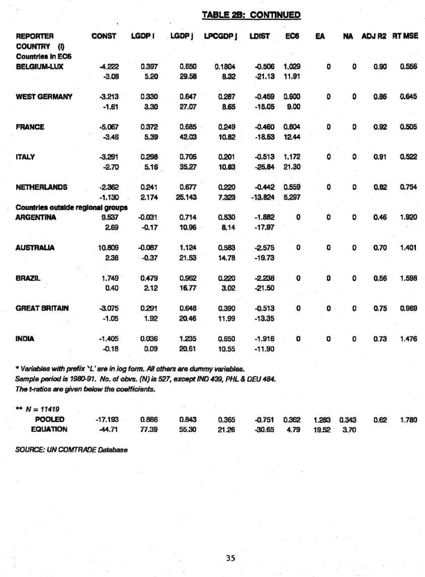
The first point to note is that compared with Table 2A, the adjusted R2_{in country-specific}

equations is consistently higher in Table 3A. This means that the addition of partner dummies increases the explanatory power of the model. Though the Table lA is not strictly comparable to Tables 2A and 3A, due to the exclusion of BORDER, one can note the steady enhancement of the explanatory power of the model from the fall in root MSE of the pooled equations. Because the results of the dummies capturing intra-regional effects (i.e., the reporter lies in the region represented by the dummy) remain qualitatively unchanged, in the following, we focus on dummies capturing the effects of outside regions (i.e., when the reporter does not lie in the region represented by the dummy).

Consider first the export equation. For countries outside East Asia, with the sole exception of Mexico, EAP has a positive and statistically significant coefficient at well above 99% level of confidence. For countries outside the EEC, the same holds true for EC6P except in the case of Japan and Singapore. For Japan, the coefficient is positive and statistically significant at 95% level of confidence while for Singapore, it is negative and statistically insignificant. For countries outside North America, the coefficient of NAP shows more ambiguity. For four out of five countries in the EEC, NAP has a negative and statistically significant coefficient at 99% level of confidence. The same also holds tue for Australia, though not for countries in East Asia. In the latter case, the coefficient is positive and statistically significant at 99% level of confidence for seven out of nine countries and negative

and statistically insignificant for the remaining two countries. In sum, controlling for other variables, countries export more to East Asia and the EEC than to countries outside the three regions represented in equation (2'). Countries in the EEC export less to North America than to countries outside the three regions in the sample.

A closer examination of Table 3A reveals that for four out of five countries in the EEC, the coefficient of EAP is larger than that of EC6P. In other words, relative to countries outside the three regions, the bias in exports in favor of East Asia is larger than the intra-regional bias! This also holds true for Canada. For U.S.A., the coefficient for EAP (1.32) is virtually the same as for NAP (1.37), implying that the bias in favor of East Asia is not much less than intra-regional bias. For the majority of countries in East Asia, the bias is the largest in favor of the EEC. For Japan and Korea the intra-regional bias and for Taiwan (China) the bias in favor of North America predominates, when compared with exports to countries outside the three regions.

In the import equations we see some evidence supporting the hypothesis of a bias against imports from North America. Oddly, the evidence points not at Japan or much of East Asia but at the EEC. Relative to countries outside the three regions, there is a favorable bias for North America but it is less than the intra-regional bias. The region that has -most to complain against Japan and Korea is the EEC whose coefficient is negative.2 4

To conclude, for countries in the EEC, on the whole, the bias in both exports and imports is positive when the partner is in the EEC or East Asia while it is negative when the

2 4_{Dhar and Panagariya 1994b presents a detailed discussion on the trade relations between}

partner is in North America. In the export equation, except in the case of Italy, the coefficient

of EAP is consistently

larger than that of EC6P, contradicting

loudly the hypothesis that East

Asian markets are closed to outside countries. Oddly enough, it is in the case of North America

that exports show a negative and statistically

significant

bias for four of the five countries in the

EEC.

4.

Conclusion

Our findings can be summarized

as follows. First, not surprisingly, the results based on

individual country equations are very different from those obtained from pooled, cross-country

equations. In some cases, the results are qualitatively different. A good example is the

coefficient

associated with distance, which shows that bilateral trade does not respond uniformly

to the proximity of nations. In cross-country

equations, our results are broadly in conformity

with the view of Anderson (1979) and others, that this coefficient is approximately

equal to

-1." Yet, in individual-country

equations, it ranges from -4.4 (Thailand, Table 2A) and -0.44

(Great Britain, Table IB). In virtually all cases the coefficient

is statistically significant

at 99%

or higher level of confidence.

Second, if there is intra-regional

bias in trade, it is to be found more in North America

and the EEC than East Asia. This result, from country-specific

equations, is broadly consistent

with that reached by Frankel (1993) from the pooled cross-country

equation. All countries in

the EEC show intra-regional

bias in exports as well as imports. The same holds true for the

United States and Canada. For 6 out of 9 countries in East Asia, exports have a statistically

25 In five out of six crosscountry equations estimated by us, the coefficient lies between

-0.89 and -0.99. In the remaining case, it is -0.75.

significant bias away from intra-regional markets.

Third, we are able to go another step beyond Frankel by testing for the openness of each region to outside countries. Out of the 45 countries in our sample, those outside North America, EEC and East Asia, serve as the control countries. The openness of each of the three regions can be compared with this control group. Our results do not support the hypothesis that East Asian markets are closed to outside countries. For example, in the export equation of U.S.A., controlling for other variables, exports to East Asia are larger than to countries in the control group. This conclusion holds true for all countries except Mexico.

Finally, in the same vein, we can consider the openness of the EEC and North America. We find that, ceterisparibus, for countries outside the EEC, exports to the EEC are larger

than

to countries in the control group (i.e., outside the three regions). For example, controlling for other variables, exports of Indonesia to EEC countries are larger than to countries in the control group. Most surprisingly and contrary to the conventional wisdom, for many countries, exports to North America are less than to countries outside the three regions! This is true for all EEC countries and Australia.

References

Aitken, N.D., 1973, "The Effect of the EEC and EFTA on European Trade: A Temporal Cross-Section Analysis," American Economic Review, Vol. 63, No. 55, pp. 881-92. Anderson, James E., 1979, "A Theoretical Foundation for the Gravity Equation," American

Economic Review Vol. 69, March, pp. 106-116.

Balassa, Bela and L. Bauwens, Changing Trade Patterns in Manufactured Goods: An Econometric Investigation, Elsevier Science Publishers, Netherlands, 1988

Bergstrand, Jeffrey H., 1989, "The Generalized Gravity Equation, Monopolistic Competition, and the Factor Proportions Theory in International Trade," Review of Economics and Statistics, pp. 143-153.

Bergstrand, Jeffrey H., 1985, "The Gravity Equation in International Trade: Some Microeconomic Foundations and Empirical Evidence," The Review of Economics and Statistics, Vol. 67, August, pp. 474-481.

Collins, Susan M. and Dani Rodrik, 1991, Eastern Europe and the Soviet Union in the World Economy, pp. 1-69, Institute for Internationial Economics, Washington D.C.

Deardorff, Alan V., 1984, "Testing Trade Theories and Predicting Trade Flows", in R.W. Jones and P.B. Kenen (eds.) Handbook of International Economics, Volume I, pp. 467-517, Amsterdam: North-Holland Publishing Co.

Dhar, Sumana and Arvind Panagariya, 1994, "Predictions of Bilateral Trade and the Gravity Equation", work in progress, International Trade Division, World Bank, Washington, D.C.

Foroutan, Faezeh and Lant Pritchett, 1991, "Intra-Sub-Saharan African Trade: Is It Too Little?" Journal of African Economies (forthcoming).

Frankel, Jeffery A., 1993, "Is Japan Creating a Yen Bloc in East Asia and the Pacific?," in J.A. Frankel and M. Kahler (eds.) Regionalism and Rivalry: Japan and the United States in Pacific Asia, Chicago: University of Chicago Press for NBER, pp. 53-87.

Hanink, Dean M., 1990, 'Linder, Again", Weltwirtschaftliches Archiv, Vol. 126, No. 2, pp. 257-267.

Havrylyshyn, 0. and L. Pritchett, 1991, "European Trade Patterns After the Transition," PRE Working Paper Series 748, The World Bank, Washington, D.C.

and Currency Zones, Federal Reserve Bank of Kansas, Jackson Hole, Wyoming, August. Linder, Steftan B., 1961, An Essay on Trade and Transformation, New York.

Linnemann, Hans, 1966, An Econometric Study of International Trade Flows, Amsterdam: North-Holland Publishing Co.

Markusen, James R., 1986, "Explaining the Volume of Trade: An Eclectic Approach," American Economic Review, Vol. 76, December, pp. 1002-1011.

Panagariya, Arvind, 1994, "East Asia: A New Trading Bloc?", Finance and Development, Vol. 31, No.1, March, Washington D.C.

Panagariya, Arvind, 1993, "Should East Asia Go Regional? No, No and Maybe", WPS 1209, October. Policy Research Dept., The World Bank, Washington D.C.

Poyhonen, P., 1963, "A Tentative Model for the Volume of Trade between Countries", Weltwirtschaftliches Archiv, Vol. 90, No. 1, pp. 93-100.

Saxonhouse, Gary R., 1992, "Pricing Strategies and Trading Blocs in East Asia," in J.A. Frankel and M. Kahler (eds.) Regionalism and Rivalry: Japan and the United States in Pacific Asia, Chicago: University of Chicago Press for NBER, pp. 89-124.

Saxonhouse, Gary R., 1993, "Trading Blocks and East Asia", in J. de Melo and A. Panagariya (eds.) New Dimensions in Regional Integration, The World Bank, Washington D.C. Srinivasan, T.N. and Gustavo Canonero, 1993, "Preferential Trade Arrangements: Estimating

the Effects on South Asian Countries", mimeo, The World Bank, Washington D.C. Tinbergen, Jan, 1962, Shaping the World Economy: Suggestions for International Economic

Policy, New York.

Thursby, Jerry G., and Marie C. Thursby, 1987, "Bilateral Trade Flows, the Linder Hypothesis, and the Exchange Risk," The Review of Economics and Statistics, August, pp. 488-495.

Wang, Z.K. and L. Alan Winters, "The Trading Potential of Eastern Europe," 1991, mimeo, Department of Economics, University of Birmingham, Birmingham.

APPENDIX I

The Countries are organized In alphabetic order of acronymns according to Region

NAME CODE ACRONYM REGION 1 CHINA 156 CHN EA 2 JAPAN 392 JPN EA

3 INDONESIA 360 IDN EA -ASEAN4

4 MALAYSIA 458 MYS EA -ASEAN4

5 PHIUPPINES 608 PHL EA -ASEAN4

6 THAILAND 764 THA EA -ASEAN4

7 HONGKONG 344 HKG EA- NIC 8 KOREA, RP 410 KOR EA - NIC

9 TAIWAN (CHINA) 8961 OAN EA -NIC

10 SINGAPORE 702 SGP EA - NIC

11 BELGIUM-WXEMBOURG 56 BLX EC6

12 GERMANY, FR 280 DEU EC6

13 FRANCE 250 FRA EC6 14 ITALY 380 ITA EC6 15 NETHERLANDS 528 NLD EC6 16 CANADA 124 CAN NA 17 MEXICO 484 MEX NA 18 USA 840 USA NA CONTROL 19 DENMARK 208 DNK EC9 20 UNITED KINGDOM 826 GBR EC9 21 IRELAND 372 IRL EC9 22 SPAIN 724 ESP EC12

23 GREECE 300 GRC EC12 24 PORTUGAL 620 PRT EC12 25 AUSTRIA 40 AUT EU 26 SWITZERLAND 756 CHE EU 27 FINLAND 246 FIN EU 28 NORWAY 578 NOR EU 29 SWEDEN 752 SWE EU 30 TURKEY 792 TUR EU 31 ARGENTINA 32 ARG LA 32 BOUVIA 68 BOL LA 33 BRAZIL 76 BRA LA 34 CHILE 152 CHL LA 35 COLOMBIA 170 COL LA 36 PERU 604 PER LA 37 PARAGUAY 600 PRY LA 38 URUGUAY 858 URY LA 39 VENEZUELA 862 VEN LA 40 AUSTRALIA 36 AUS OCN

41 NEW ZEALAND 554 NZL OCN 42 BANGLADESH 50 BGD SA

43 INDIA 356 IND SA 44 SRI LANKA 144 LKA SA 45 PAKISTAN 586 PAK SA

APPENDIX 2

Years: 1980-1992 with the provision to expand to 1958-1968 for the comparison with EC.

Trade: XJ (M'J

)

reporter and partner for 1980-1992 from the COMTRADE database of UN Statistical Organization, Geneva.

GDP: GDPi, GDPj - GDP in US dollar of the reporter and partner for 1980-1992. GDP per capita: PCGDPi, PCGDPj - GDP per capita in US dollar of the reporter and

partner for 1980-1992.

* Nominal GDP from the National Accounts database of the World Bank which

uses the Atlas Method. (Atlas Method - The data at current prices are converted from the local currency to US dollars using a conversion factor other than the official for each year, when the official exchange rate is greatly distorted.) Populations of the reporter and partner for 1980-1992 from the IEC Social and Demographic Indicators database were then used to obtain the nominal GDP per capita

* Real GDP per capita from the Summers Heston (1992) database for 1980-1988. Populations of the reporter and partner for 1980-1988 from the same database

were then used to obtain the real GDP.

Size: areai - Land area of the reporter in '000 sq. km. from the IEC Social and

Demographic Indicators database.

Distarce: di - The straight-line distance between major ports of entry of reporter and partner from Linneman (1966).

BORDER: b', - Dummy = 1 if the countries i and j share a common border, 0 otherwise. Regional Arrangements: EC6, EA, NA - Dummy = 1 if both reporter and partner are

members of a regional block, 0 otherwise.

EC6P, EAP, NAP - Dummy = 1 if partner is a member of a regional block, 0 otherwise.

TABLE I A: GRAVITY MODEL OF BILATERAL TRADE

BEFORE THE INTRODUCTION OF REGIONAL DUMMIES"

LHS VARIABLE: LOG OF TOTAL EXPORTS *

REPORTER CONST LGDP I LGDP J LPCGDPj LDIST BORDER ADJ R2 RT MSE COUNTRY (I) Countrles In EA HONG KONG 1.073 0.061 0.614 0.648 -0.884 1.766 0.69 1.165 0.45 0.43 13.33 15.10 -14.12 5.69 INDONESIA -24.421 1.835 1.401 0.636 -3.504 -3.829 0.75 1.871 -2.14 2.91 20.34 7.62 -26.76 -14.00 JAPAN 8.164 0.114 0.695 0.279 -1.308 0 0.85 0.617 5.69 1.79 26.51 12.36 -31.81 KOREA -13.726 0.740 0.396 0.577 -0.033 0 0.28 2.128 -3.60 4.16 4.19 5.13 -0.14 MALAYSIA 4.862 0.666 1.124 0.198 -2.095 -1.943 0.81 1.122 -1.23 2.88 27.88 5.24 -29.71 -5.63 TAIWAN (CHINA) -10.562 0.821 0.323 0.819 -0.627 0 0.37 1.980 -3.23 4.98 3.29 7.53 -3.76 PHILIPPINES 15.881 -0.883 1.044 0.697 -1.865 0 0.73 1.538 1.83 -1.76 18.07 10.79 -18.80 SINGAPORE -6.793 0.305 0.925 0.357 -0.809 1.959 0.35 2.493 -1.08 0.95 14.26 4.40 -2.09 1.21 THAILAND -9.139 1.094 1.068 0.716 -2.942 -0.454 0.76 1.584 -2.95 6.22 22.92 13.63 -27.38 -2.27 Countries In NA CANADA -2.415 -0.250 0.965 0.004 0.228 2.526 0.82 0.745 -0.92 -2.03 34.28 0.16 2.20 11.88 MEXJCO 18.289 -0.263 1.232 -0.119 -2.865 -1.161 0.52 2.142 2.31 -0.66 19.24 -1.90 -14.44 -3.75 USA -0.276 -0.069 0.750 0.133 0.171 2.003 0.75 0.736 -0.09 -0.52 31.48 4.07 1.59 11.53

TABLE IA: CONTINUED

REPORTER CONST LGDP I LGDP I LPCGDPj LDIST BORDER ADJ R2 RT MSE COUNTRY (I) Countries in EC6 BELGIUM-LUX -2.925 0.327 0.785 0.063 -0.706 0.546 0.86 0.741 -1.53 3.13 25.94 1.69 -20.51 6.08 WEST GERMANY -2.687 0.359 0.724 0.149 -0.622 0.264 0.91 0.537 -1.55 4.27 35.78 5.78 -20.78 3.55 FRANCE -2.068 0.316 0.722 0.092 -0.639 0.551 0.91 0.534 -1.33 4.06 35.53 3.62 -21.68 8.76 ITALY -3.347 0.334 0.757 0.279 -0.789 -0.336 0.89 0.597 -2.43 5.22 34.98 10.98 -17.34 -3.10 NETHERLANDS 3.723 0.083 0.653 0.157 -0.742 0.714 0.87 0.687 1.92 0.80 26.67 5.62 -27.43 10.45

Countries outside regional groups

ARGENTINA -5.912 0.487 0.868 -0.116 -0.844 1.739 0.46 1.423 -2.06 3.44 19.05 -2.14 -6.65 5.68 AUSTRALIA 15.673 0.024 1.270 0.214 -3.350 0 0.74 1.327 3.44 0.10 24.39 4.88 -24.55 BRAZIL 2.204 0.095 0.792 0.065 -0.809 1.152 0.69 0.815 0.84 0.73 27.57 1.90 -7.77 6.72 GREAT BRITAIN 0.023 0.187 0.642 0.261 -0.516 1.443 0.76 0.859 0.01 1.45 22.88 6.84 -13.22 15.30 INDIA -0.122 0.622 0.848 0.708 -2.648 -0.871 0.80 1.031 -0.02 2.27 23.33 14.70 -32.98 -2.67

* Variables with prefix 'L' are in log form. All others are dummy variables.

Sample period is 1980-91. No. of obvs. (N) is 527, except PHL 439, DEU and IND 484. t-ratios are given below the coefficients.

** N=11419

POOLED -12.379 0.831 0.837 0.174 -0.987 0.349 0.59 1.781 EQUATION -27.64 72.22 55.60 9.58 -29.89 3.72

TABLE 1 B: GRAVITY MODEL OF BILATERAL TRADE

BEFORE THE INTRODUCTION OF REGIONAL DUMMIES**

LHS VARIABLE: LOG OF TOTAL IMPORTS *

REPORTER CONST LGDP I LGDP j LPCGDP LDIST BORDER ADJ R2 RT MSE COUNTRY (I) Countries In EA HONG KONG -5.486 0.472 0.935 0.598 -1.574 0.913 0.76 1.347 -1.96 2.81 17.24 10.70 -22.06 3.99 INDONESIA -22.229 1.207 1.342 0.672 -2.255 -1.875 0.75 1.600 -2.22 2.21 24.69 14.45 -20.28 -7.51 JAPAN 2.743 0.250 0.858 0.145 -1.293 0 0.77 0.861 1.37 2.80 30.72 4.01 -19.84 KOREA -16.656 0.594 0.627 0.762 -0.082 0 0.39 2.280 -4.13 3.12 6.71 7.06 -0.35 MALAYSIA -8.686 0.697 0.954 0.476 -1.644 -0.478 0.59 1.547 -1.61 2.19 20.73 11.30 -15.56 -1.49 TAIWAN (CHINA) -14.281 0.732 0.512 0.874 -0.513 0 0.42 2.090 -4.08 4.03 5.43 8.03 -3.10 PHIUPPINES -9.121 0.450 1.116 0.855 -1.930 0 0.66 2.033 -0.82 0.69 19.91 10.43 -18.02 SINGAPORE -10.290 0.310 1.005 0.600 -0.840 2.373 0.45 2.377 -1.73 1.03 16.68 8.25 -2.30 1.55 THAILAND -6.534 0.550 1.203 0.631 -2.281 0.436 0.77 1.455 -2.06 3.24 21.37 13.57 -21.07 2.79 Countries In NA CANADA -13.782 0.333 0.877 0.298 0.107 1.977 0.78 0.910 -4.19 2.00 24.75 8.80 0.85 7.84 MEXICO -26.801 1.385 0.821 0.383 -0.867 1.422 0.46 2.024 -3.57 3.68 17.62 7.61 -4.25 5.20 USA -15.556 0.428 0.829 0.144 0.508 2.471 0.71 0.880 -4.18 2.52 28.25 3.73 3.53 11.06

TABLE I1B: CONTINUED

REPORTER CONST LGDP I LGDP J LPCGDP j LDIST BORDER ADJ R2 RT MSE COUNTRY (I) Countries In EC6 BELGIUM-LUX -4.399 0.383 0.663 0.188 -0.489 1.165 0.90 0.559 -0.20 5.01 31.16 8.67 -19.81 12.30 WEST GERMANY -3.105 0.322 0.671 0.270 -0.489 0.228 0.86 0.658 -1.52 3.18 29.64 8.26 -13.50 2.88 FRANCE -4.829 0.370 0.693 0.237 -0.494 0.522 0.91 0.521 -3.20 5.23 42.52 10.26 -19.23 6.63 ITALY -2.148 0.255 0.754 0.213 -0.653 -0.166 0.88 0.601 -1.51 3.86 35.09 10.63 -18.04 -1.61 NETHERLANDS -2.811 0.226 0.689 0.235 -0.395 1.219 0.83 0.735 -1.38 2.10 27.62 7.72 -12.53 13.68

Countrles outside regional groups

ARGENTINA -5.183 -0.120 0.740 0.693 -0.278 4.173 0.53 1.788 -1.49 -0.68 13.47 10.26 -1.40 9.17 AUSTRALIA 10.809 -0.087 1.124 0.583 -2.575 0 0.70 1.401 2.38 -0.37 21.53 14.78 -19.73 BRAZIL -4.425 0.378 1.005 0.312 -1.507 1.490 0.58 1.560 -1.01 1.72 17.92 4.07 -8.96 4.79 GREAT BRITAIN -3.621 0.265 0.670 0.398 -0.445 1.174 0.75 0.957 -1.26 1.77 21.25 12.36 -11.75 12.83 INDIA -1.028 0.091 1.302 0.514 -2.087 -1.251 0.73 1.460 -0.13 0.23 20.69 7.63 -12.66 -4.73

* Variables with prefix 'L are in log form. All others are dummy variables.

Sample period is 1980-91. No. of obvs. is 527, except IND 439, PHL and DEU 484.

The t-ratios are given below the coefficients.

** N = 11419

POOLED -14.738 0.829 0.867 0.321 -0.910 0.326 0.64 1.803 EQUATION -32.87 70.19 58.42 17.84 -28.18 3.40

TABLE 2A: GRAVITY MODEL OF BILATERAL TRADE

DUMMIES: REPORTER AND PARTNER COUNTRIES ARE BOTH IN THE REGION ** WrrHOUT DUMMY FOR COMMON BORDER

LHS VARIABLE: LOG OF TOTAL EXPORTS

REPORTER CONST LGDP I LGDP j LPCGDP J LOIST EC6 EA NA ADJ R2 RT MSE

COUNTRY 0) Countries In EA HONG KONG 4.293 0.W46 0.651 0.633 -1.271 0 -0.835 0 0.66 1.178 1.64 0.32 14.20 13.88 -10.25 -3.17 INDONESIA -25.084 1.B19 1.455 0.596 -3.458 0 -0.701 0 0.73 1.932 -217 2.83 22.32 7.26 -16.77 -2.15 JAPAN 3.574 0.115 0.718 0.251 -0.830 0 0.927 0 0.86 0.587 2.42 1.93 28.55 12.58 -13.25 8.08 KOREA -25.209 0.742 0.476 0.480 1.141 0 2.816 0 0.33 2.048 4.98 4.34 5.68 4.79 2.56 4.95 MALAYSIA -7.554 0.665 1.160 0.161 -1.B22 0 -0.306 0 0.79 1.173 -1.80 0.74 27.87 4.18 -19.91 -1.70 TAIWAN (CHINA) -14.593 0.834 0.335 0.774 0.191 0 1.068 0 0.38 1.971 -3.67 5.07 3.48 7.57 -0.66 2.57 PHIUPPINES 16.393 -0.889 1.045 0.701 -1.915 0 -0.118 0 0.73 1.539 1.85 -1.77 18.09 10.82 -9.30 -0.31 SINGAPORE -1.732 0.274 0.919 0.424 -1.363 0 -0.960 D 0.35 2490 -0.31 0.86 12.42 4.76 -6.71 -2.96 THAILAND 4.145 1.007 1.110 0.826 -4.410 0 -2.958 0 0.80 1.455 1.2B 5.89 25.74 16.63 -24.16 -11.83 Countries In NA CANADA 0.11 B -0.250 0.993 -0.035 -0.099 0 0 0.859 0.80 0.782 0.04 -1.90 36.12 -1.15 -0.93 3.48 MEXICO 17.857 -0.260 1.211 -0.104 -2-792 0 0 -0.490 0.52 2145 2.26 -0.65 19.77 -1.68 -14.96 -1.98 USA -0.276 -0.069 0.750 0.133 0.171 0 0 2.004 0.75 0.736 -0.09 -0.52 31.48 4.07 1.59 11.53

TABLE 2A: CONTINUED

REPORTER CONST LGDPI LGDPJ LPCGDPj LDIST EC6 EA NA ADJ 2 RT MSE

COUNTRY (I) Countries In EC6 BELGIUM-LUX -3.034 0.337 0.768 0.06o1 -0.685 0.699 0 0 0.87 0.731 -1.61 3.25 24.75 1.85 -21.78 9.42 WESTGERMANY -2.472 0.365 0.711 0.156 -0.639 0.314 0 0 0.91 0.535 -1.44 4.35 33.99 5.94 -24.24 4.60 FRANCE -1.882 0.313 0.727 0.093 -0.662 0.463 0 0 0.91 0.541 -1.20 3.98 35.35 3.56 -21.95 6.48 ITALY 4.317 0.357 0.728 0.272 -0.691 0.663 0 0 0.90 0.577 -3.34 5.84 34.80 10.78 -21.16 10.88 NETHERLANDS 3.592 0.099 0.627 0.164 -0.713 0.734 0 0 0.88 0.678 1.871 0.950 24.286 5.916 -26.861 9.740

Countries outside regional groups

ARGENTINA 0.223 0.524 0.858 -0.184 -1.513 0 0 0 0.44 1.452 0.08 3.62 17.95 -3.55 -21.75 AUSTRALA 15.673 0.024 1.270 0.214 -3350 0 0 0 0.74 1.327 3.44 0.10 24.39 4.88 -24.55 BRAZIL 6.979 0.173 0.759 -0.005 -1.373 0 0 0 0.65 0.859 2.60 1.28 23.97 -0.17 -19.49 GREAT BRITAIN 0.695 0.219 0.614 0.251 -0.600 0 0 0 0.75 0.B80 0.27 1.66 21.41 6.48 -14.79 INDIA -0.389 0.584 0.802 0.802 -2.529 0 0 0 0.80 1.043 -0.07 210 24.43 18.84 -24.06

* Variables with prefix 'L' are in log form. All others are dummy variables.

Sample period is 1980-91. No. of obvs. (N) is 527, except PHL 439, DEU & IND 484

t-ratios are given below the coefficients. N =11419

POOLED -13.615 0.864 0.825 0.200 -0.918 0.153 0.740 0.143 0.59 1.774

EQUATION -36.16 77.66 53.26 11.49 -37.26 2.02 10.55 1.73

TABLE 25: GRAVITY MODEL OF BILATERAL TRADE

DUMMIES: REPORTER AND PARTNER COUNTRIES ARE BOTH IN THE REGION **

WITHOUT DUMMY FOR COMMON BORDER

LHS VARIABLE: LOG OF TOTAL IMPORTS'

REPORTER CONST LGDPI LGDPj LPCGDPI LDIST EC6 EA NA ADJ R2 RT MSE

COUNTRY (0 Countries In EA HONG KONG -6.456 0.478 0.967 0.552 -1.498 0 0,295 0 0.76 1.351 -2.13 2.82 19.56 10.14 -11.65 1.08 INDONESIA -26.874 1.251 1.336 0.638 -1.786 0 0.675 0 0.75 1.611 -2.66 2.29 23.38 13.55 -10.14 2.79 JAPAN 4.581 0.253 0.894 0.099 -0.531 0 1.479 0 0.80 0.806 -2,11 3.01 32.42 2.29 -4.17 7.25 KOREA -34.812 0.597 0.754 0.609 1.774 0 4.452 0 0.49 2.087 -7.23 3.38 9.33 6.59 4.35 8.28 MALAYSIA -12993 0.744 0.911 0.474 -1.171 0 1.160 0 0.67 1.520 -2.45 2.40 18.75 12.22 -11.25 7.44 TAIWAN (CHINA) -24.915 0.766 0.542 0.756 0.638 0 2.818 0 0.46 2.018 -6.24 4.34 5.97 7.43 2.27 6.98 PHILIPPINES -15.726 0.517 1.114 0.811 -1.286 0 1.541 0 0.66 2.014 -1.41 0.80 19.60 10.62 -5.80 3.48 SINGAPORE -7.745 0.299 0.953 0.684 -1.081 0 0.122 0 0.45 2391 -1.47 0.98 13s58 802 -5.28 0.40 THAILAND -1.237 0.519 1.210 0.680 -2.860 0 -1.065 0 0.78 1.438 -0.37 3.07 21.59 14.30 -13.82 -4.02 Countries In NA CANADA -13.448 0.328 0.874 0.311 0.075 0 0 1.497 0.78 0.901 -4.17 1.98 25.56 9.49 0.68 8.54 MEXICO -26.601 1.3B7 0.834 0.367 -0.905 0 0 0.895 0.46 2.025 -3.55 3.8 18.50 7.44 4.59 4.20 USA -15.556 0.428 0.830 0.145 0.509 0 0 2.472 0.71 0.80 4.18 2.52 28.25 3.73 3.55 11.06

TABLE 2B: CONTINUED

REPORTER CONST LGDP I LGDP J LPCGDP J LDIST EC6 EA NA ADJ R2 RT MSE

COUNTRY (0 Countries In EC6 BELGIUM-LUX -4.222 0.397 0.650 0.1804 -0.506 1.029 0 0 0.90 0.556 -3.08 5.20 29.58 8.32 -21.13 11.91 WEST GERMANY -3.213 0.330 0.647 0.287 -0.459 0.600 0 0 0.86 0.645 -1.61 3.30 27.07 8.65 -15.05 9.00 FRANCE -5.067 0.372 0.685 0.249 -0.460 0.604 0 0 0.92 0.505 -3.45 5.39 42.03 10.82 -18.53 12.44 ITALY -3.291 0.298 0.705 0.201 -0.513 1.172 0 0 0.91 0.522 -2.70 5.16 35.27 10.83 -25.84 21.30 NETHERLANDS -2.362 0.241 0.677 0.220 -0.442 0.559 0 0 0.02 0.754 -1.130 2.174 25.143 7.323 -13.824 5.297

Countries outside regional groups

ARGENTINA 9.537 -0.031 0.714 0.530 -1.882 0 0 0 0.46 1.920 2.69 -0.17 10.96 8.14 -17.97 AUSTRALIA 10.809 -0.087 1.124 0.583 -2.575 0 0 0 0.70 1.401 2.38 -0.37 21.53 14.78 -19.73 BRAZIL 1.749 0.479 0.962 0.220 -2.238 0 0 0 0.56 1.598 0.40 2.12 16.77 3.02 -21.50 GREAT BRITAIN -3.075 0.291 0.648 0.390 -0.513 0 0 0 0.75 0.969 -1.05 1.92 20.46 11.99 -13.35 INDIA -1.405 0.036 1.235 0.650 -1.916 0 0 0 0.73 1.476 -0.18 0.09 20.61 10.55 -11.90

'Variables with prefix 'L' are in log form. All others are dummy variables.

Sample period is 1980-91. No. of obvs. (N) is 527, except IND 439, PHL & DEU 484. The t-ratios are given below the coefficients.

N = 11419

POOLED -17.193 0.865 0.843 0.365 -0.751 0.362 1.283 0.343 0.62 1.780

EQUATION -44.71 77.39 55.30 21.26 -30.65 4.79 19.52 3.70

TABLE MA: GRAVITY MODEL OF BILATERAL TRADE

DUMMIES: ONLY PARTNER COUNTRY IS IN THE REGION*'

WITHOUT DUMMY FOR COMMON BORDER LH8 VARIABLE: LOG OF TOTAL EXPORTS'

REPORTER CONST LODP I LGDP J LPCGDP I LDI9T ECOP EAP NAP ADJ R2 RT MBE COUNTRY (I) Countrles In EA HONG KONG 4.910 0.109 0.561 0.627 -1.294 0.670 -0.727 0.679 0.69 1.161 1.90 0.77 10.43 14.12 -10.65 4.34 -2.93 2.84 INDONESIA -26.994 2.066 1,296 0.569 3.440 1.333 -0.391 1.178 0.74 1.994 -2.38 3.27 17.41 7.10 -16.48 5.68 -1.22 5.51 JAPAN 3.531 0.139 0.677 0.245 0.803 0.192 1.010 0.3B7 0.86 0.582 2.40 2.37 24.35 12-44 -1239 1.86 8.49 3.26 KOREA -24.272 0.802 0.345 0.484 1,151 0.423 3.033 1.568 0.35 2.023 -4.88 4.73 3.55 4.77 2.58 2.77 5.20 5.11 MALAYSIA -8.319 0.742 1.119 0.134 -1.790 0.767 -0.164 -0.130 0.80 1.152 -2.02 3.10 22.20 3.62 -19.59 4.03 -0.88 -0.72 TAIWAN (CHINA) -12.792 0.937 0.130 0.767 -0.215 1.132 1.356 1.987 0.41 1.915 -3.38 5.77 1.22 7.56 -076 7.84 3.19 6.47 PHILUPPINES 14.150 -0.602 0.907 0.671 -1.942 1.306 0.090 0.858 0.75 1.498 1.65 -1.23 12.72 10.66 -9.44 5.93 0.25 3.29 SINGAPORE -1.903 0.266 0.936 0.419 -1.357 -0.003 -0.977 -0.241 0.35 2.494 -0.35 0.62 10.97 4.66 -6.67 -0.02 -2.67 -1.32 THAILAND 3.800 1.109 1.007 0.752 4.350 1.316 -2.667 0.330 0.81 1.412 1.22 6.74 19.09 16.63 -24.51 5.81 -10.94 1.27 Countries In NA CANADA 4.645 -0.159 0.899 -0.044 -0.653 D.187 0.985 0.722 0.84 0.702 1.96 -1.37 33.43 -1.54 -5.52 1.64 12.67 3.58 MEXICO 16.455 -0.231 1.195 -0.138 -2628 0.439 -0.360 -0.295 0.52 2.139 2i10 -0.58 16.50 -1.85 -15.63 2.66 -0.98 -1.05 USA 5,533 0.055 0.638 0.109 -0.604 0.471 1.315 1.368 0.84 0.586 2.27 0.53 27.86 4.07 -. 10 5.33 17.51 9.28