Bank of Canada staff working papers provide a forum for staff to publish work-in-progress research independently from the Bank’s Governing Council. This research may support or challenge prevailing policy orthodoxy. Therefore, the views expressed in this paper are solely those of the authors and may differ from official Bank of Canada views. No responsibility for them should be attributed to the Bank.
Staff Working Paper/Document de travail du personnel 2015-45
Exchange Rate Fluctuations and
Labour Market Adjustments in
Canadian Manufacturing
Industries
Bank of Canada Staff Working Paper 2015-45
December 2015
Exchange Rate Fluctuations and
Labour Market Adjustments in
Canadian Manufacturing Industries
by
Gabriel Bruneau1 and Kevin Moran2
1Financial Stability Department Bank of Canada
Ottawa, Ontario, Canada K1A 0G9 gbruneau@bankofcanada.ca
2Department of Economics Université Laval, Quebec
kmoran@ecn.ulaval.ca
Acknowledgements
The authors would like to thank Shutao Cao, Yaz Terajima, Mario Crucini and one anonymous referee for very useful suggestions. The authors would also like to thank Brian Peterson, Benoît Carmichael, Natalya Dygalo, Marc Henry, Lynda Khalaf, Benoît Perron and Robert Amano and participants at a seminar at the Bank of Canada and at the annual meeting of the Canadian Economics Association. Finally, the authors would like to thank Lucia Chung for excellent research assistance.
Abstract
We estimate the link between exchange rate fluctuations and the labour input of Canadian manufacturing industries. The analysis is based on a dynamic model of labour demand, and the econometric strategy employs a panel two-step approach for cointegrating regressions. Our data are drawn from a panel of 20 manufacturing industries from the KLEMS database and cover a long sample period that includes two full cycles of appreciation and depreciation of the Canadian dollar. Our results indicate that exchange rate fluctuations have significant long-term effects on the labour input of Canada’s manufacturing industries, that these effects are stronger for trade-oriented industries, and that these long-term impacts materialize only gradually following shocks.
JEL classification: E24, F14, F16, F31, F41, J23
Bank classification: Exchange rates; Exchange rate regimes; Econometric and statistical methods; Labour markets; Recent economic and financial developments
Résumé
Nous examinons le lien entre les variations du taux de change et celles du facteur travail dans les industries manufacturières canadiennes. Notre analyse est fondée sur un modèle dynamique de la demande de travail, et notre méthode économétrique met à profit une approche en deux étapes pour données de panel, afin d’estimer les relations de cointégration. Nos données sont tirées d’un panel de 20 industries manufacturières provenant de la base de données KLEMS et couvrent une longue période comprenant deux cycles complets d’appréciation et de dépréciation du dollar canadien. Nos résultats montrent que les fluctuations du taux de change ont d’importantes répercussions à long terme sur le facteur travail des industries considérées, que ces effets sont plus marqués dans les secteurs à vocation exportatrice et que ces incidences à long terme ne se matérialisent que progressivement à la suite de chocs.
Classification JEL : E24, F14, F16, F31, F41, J23
Classification de la Banque : Taux de change; Régimes de taux de change; Méthodes économétriques et statistiques; Marchés du travail; Évolution économique et financière récente
Non-Technical Summary
The labour market response to fluctuations in the exchange rate has drawn strong interest over the past decade, as concerns emerged that the higher value of the Canadian dollar would cause protracted declines in manufacturing jobs. Conversely, the more recent period of depreciation of the currency has led to conjecture about whether manufacturing in Canada will rebound.
This paper provides a quantitative analysis of the link between exchange rate fluc-tuations and the labour input of manufacturing industries. Specifically, we ask the following questions: (i) What are the long-term impacts of changes to real exchange rates on manufacturing hours and jobs? (ii) How fast do the adjustments towards these long-term impacts take place? To address these questions, the paper formulates a model of labour demand and estimates it using data spanning from 1961 to 2008, thus covering all the major shifts in the real value of Canada’s currency over the past 50 years.
We report four main findings. First, exchange rate fluctuations have sizeable effects on hours worked and jobs in Canadian manufacturing industries. Second, these adjustments occur relatively slowly. Third, these effects are stronger for industries with a high exposure to international trade. Finally, we document that the enactment of two major trade deals between Canada and its North American partners has had significant negative impacts on the labour input of Canadian manufacturing firms.
1
Introduction
The influence of exchange rates on Canadian manufacturing industries has attracted much attention historically. The past decade’s sustained appreciation of the Canadian dollar relative to its U.S. counterpart has proven to be no exception, as concerns were raised that the high value of the Canadian dollar was contributing to protracted declines in manufacturing jobs. Conversely, the more recent period of depreciation of the currency has led to conjecture about whether manufacturing in Canada will rebound.
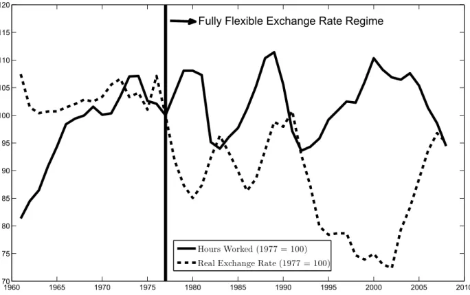
Figure 1 illustrates the evolution of the real value of the Canadian dollar and that of total hours worked in manufacturing between 1961 and 2008.1 The figure shows that the pronounced cycles of depreciation and appreciation experienced by the Canadian dollar over the past 50 years appear to have been negatively correlated with hours worked in manufacturing. For example, the 1990s were characterized by a steady depreciation of the Canadian dollar and, throughout this period, hours worked in manufacturing were increasing. Conversely, the early 2000s witnessed a rapid appreci-ation of the currency at the same time as important retrenchments in manufacturing hours occurred.
This paper provides a quantitative analysis of the link between exchange rate fluc-tuations and the labour input of manufacturing industries. We ask the following questions: (i) What are the long-term impacts of changes to real exchange rates on manufacturing hours and jobs? (ii) How fast do the adjustments towards these long-term impacts take place? To address these questions, the paper formulates a dynamic labour-demand model and estimates it using a panel cointegrating approach with an error-correcting mechanism. The data used to estimate the model are from KLEMS,2
1The real effective exchange rate measure is from a database created byBruegel that provides real effective exchange rates for several countries. Nominal rates are deflated by pairwise relative CPIs and are weighted by trading importance; an increase represents an appreciation of the Canadian dollar. Hours worked is for all manufacturing industries and is from the KLEMS database. Details on the data used in this paper are presented below.
an industry-level database of panel data organized under the North American Industry Classification System (NAICS) that spans the period from 1961 to 2008, covering all major shifts in the real value of Canada’s currency over the past 50 years.
We report four main findings. First, exchange rate fluctuations have sizeable effects on hours worked and jobs in Canadian manufacturing industries. Under our benchmark specification, a 10 percent real depreciation of the Canadian dollar is associated with a 3 percent increase in hours worked and an increase just under that for the number of jobs. Second, these adjustments occur relatively slowly, with about 13 percent of the gap between actual and targeted labour (defined below) closed each year. Third, these effects are stronger for industries with a high exposure to international trade. Finally, we document that the enactment of two major trade agreements between Canada and its North American trading partners has had significant negative impacts on the labour input of Canadian manufacturing firms.
An earlier related paper is Leung and Yuen (2007), who also study the impact of exchange rate fluctuations on the labour input of Canadian manufacturing firms. The current paper offers two important contributions relative to Leung and Yuen (2007). First, we use a substantially longer sample (1961-2008) that allows our analysis to cover all important shifts in the external value of the Canadian dollar over the past 50 years. Second, this longer dataset permits the use of an econometric methodology focusing on the long-term adjustments to exchange rate shifts. To this end, we first estimate a (panel) cointegrating relationship between the labour input of manufacturing firms, the real effective exchange rate, and other economic variables. Once the cointegrating vector is established, we then evaluate the speed at which gaps between actual and targeted values of variables are corrected.3 Our analysis can thus bring to bear information contained in both the long-term relationship between exchange rates and labour, as well as in the dynamic adjustment towards that long-term relationship. Other related work includes Campa and Goldberg (2001), who study the adjustment
3The shorter sample (1981-1997) available to Leung and Yuen (2007) prevented them from focusing on long-term adjustments, and they did not use cointegration techniques.
1960 1965 1970 1975 1980 1985 1990 1995 2000 2005 2010 70 75 80 85 90 95 100 105 110 115 120
Fully Flexible Exchange Rate Regime
Hours Worked (1977 = 100) Real Exchange Rate (1977 = 100)
Figure 1: Real Effective Exchange Rate of the Canadian dollar versus
Hours Worked in Manufacturing (All Industries, 1977=100, 1961-2008).
of American manufacturing firms to U.S.-dollar fluctuations and find no significant impact on employment and hours worked. By contrast, Dekle (1998) reports that changes in the external value of the yen have significant effects on Japanese manu-facturing employment. Burgess and Knetter (1998), studying a set of industrialized countries, report that exchange rate fluctuations have very small impacts on man-ufacturing employment in some countries, such as Germany and France, but have significant impacts in others, including the U.S., Canada and the U.K. None of these studies apply econometric strategies designed to allow cointegrated variables and identify long-term adjustments.
The remainder of this paper is organized as follows. Section 2 presents our theoretical model and the empirical specification. Section 3 introduces the data employed in the estimation, which are taken from the most recent release of the KLEMS database.
Section 4 presents the methodology and Section 5 reports our estimation results and assesses their robustness through an extensive sensitivity analysis. Finally, Section 6 concludes. A detailed description of all data used is provided in the Appendices.
2
Model
This section develops an econometric model to analyze the long- and short-term im-pacts of exchange rate fluctuations on the labour input of Canadian manufacturing firms. The model assumes that Canada’s manufacturing firms operate in monopo-listically competitive environments in both their domestic and foreign markets. Ac-cordingly, firms maximize profits by choosing their product’s relative price, subject to a production function, to input prices for which they are price-takers and to labour adjustment costs.
In this context, assume that worldwide demand for the product of firm i is expressed as
yi,td =xi,tp−i,tθ, (1)
where pi,t is the firm’s relative price, θ is the price elasticity of demand, and xi,t
indexes the overall demand for goods. The product-demand shifter xi,t first depends
on the real exchange rate st between Canada and its trading partners. An increase in
st represents a real appreciation that reduces the ability of domestic firms to export
profitably and allows foreign imports to enter more easily into Canada. We therefore expect st to have a negative impact on xi,t. Next, xi,t depends on worldwide demand
for Canadian goods ytall, which we measure by an aggregate of Canada’s GDP and that of its trading partners.4 We expect a positive impact from yall
t . Finally, we allow
xi,t to be affected by the enactment of two major trade agreements (the Canada-U.S.
Free Trade Agreement in 1989 and the North American Free Trade Agreement in 1994), as well as the switch to floating exchange rates between the Canadian and U.S.
4The notationyall
t reflects the influence of both domestic and foreign demand (the sum ofYtand
Yt∗ in the model derived in Appendix C). Our empirical work measures yall
t as the G7 aggregate
of real GDPs produced by the OECD, but our results are robust to alternative measures of world demand for Canada’s manufacturing products.
dollars in the 1970s.
Next, assume that the production function for firm i is
yi,t =ai,tF (li,t, ki,t, iii,t), (2)
whereai,t is multifactor productivity in industryiat time t,li,t is a (quality-weighted)
labour input,ki,t is the capital input,iii,t is the input of intermediate goods, and F(·)
is a constant returns-to-scale production function.5 The price of labour in industry
i is denoted by wi,t, while the prices for capital and intermediate inputs are pKi,t and
pIIi,t, respectively.
Consider first a frictionless choice of the labour input, when no adjustment costs are present. Maximizing profits subject to (1) and (2) yields the following expression:
lnl∗i,t = αi,0+α1lnwi,t+α2lnpi,tK +α3lnpIIi,t+α4lnai,t+α5lnst+
α6lnytall+αi,7CU SF T At+αi,8N AF T At+αi,9F EXt+εLTi,t , (3)
where CU SF T At and N AF T At are time dummies controlling for the two trade
agreements, while F EXt indexes the transition towards floating exchange rates in the
1970s. Appendix C derives (3) in the case of a two-input CES production function. It shows that the own-price elasticity parameterα1 must be negative, but that the signs
of α2 and α3 can vary according to the strength of substitution between labour and
other inputs. It also describes how α4 > 0, α5 < 0 and α6 >0.6 In expression (3),
fluctuations in the real exchange rate can affect labour input through two channels: first, a direct (demand) effect that arises because exchange rate fluctuations affect the demand of trade-oriented firms (the parameter α5); second, an indirect effect
that arises if one of the production inputs is imported, so that real exchange rate
5The KLEMS database is also constructed using a constant returns-to-scale framework.
6Note that the coefficients on prices and aggregate variables are common across industries, while the time dummies are allowed to have industry-specific effects. Specifications in previous versions of the research included an industry-specific time trend to account for the possibility of a secular decline in manufacturing sector activities and the results were quantitatively similar.
fluctuations affect its relative price and thus also labour demand through a substitution channel. Such an effect is most likely to be sizeable for Canadian manufacturing firms in the case of the capital input.
Starting with Nickell (1987), a large body of literature has assumed that adjustment costs prevent the frictionless labour input li,t∗ in (3) from being obtained. Instead, this literature (Burgess and Knetter, 1998; Dekle, 1998; Campa and Goldberg, 2001; Leung and Yuen, 2007) derives a partial-adjustment process towards the long-run “target” labour input l∗i,t, as in
lnli,t =νlnli,t−1+ (1−ν) lnl∗i,t,
or, written differently,
∆ lnli,t =−(1−ν) lnli,t−1−lnl∗i,t
, (4)
where(1−ν) is the speed of adjustment towards the long-run targeted labour input. Since our data are shown to be integrated and cointegrated, a natural interpretation of equations (3) and (4) is that of a cointegrating relationship with an error-correction mechanism. Accordingly, our econometric strategy, discussed in detail below, involves first estimating the long-run relationship (3) and then the following generalized version of (4):
∆ lnli,t =−(1−ν) lnli,t−1−lnl∗i,t
+ p X s=1 δs,iy ∆ lnli,t−s+ p X s=0
δs,iX∆ lnXi,t+εSTi,t , (5)
where Xi,t = {wi,t, pKi,t, pIIi,t, ai,t, st, ytall}. Our estimation strategy uses the methods
described in Breitung (2005) and Pesaran, Shin, and Smith (1999), which allow the intercepts (and other coefficients on deterministic regressors), short-run coefficients and error variances to differ across industries, but constrain the long-run coefficients
to be the same.7
3
Data
A balanced panel of annual data for the Canadian manufacturing sector is used to estimate equations (3) and (5). The database includes both industry-specific and aggregate data and spans from 1961 to 2008.
The industry-specific data are from the KLEMS database. KLEMS, from Statistics Canada’s Canadian Productivity Accounts, provides annual data on prices and quan-tities of output, as well as on capital, labour and intermediate inputs for all Canadian industries. The database is organized under the NAICS, and the data we use pertain to the 20 manufacturing industries at the 3-digit industry level.8 KLEMS provides us with data for the quality-weighted labour inputli,t, the hours worked hi,t, the number
of jobs ji,t, multifactor productivity ai,t, and, when used in combination with the
Industrial Product Price Indexes, the relative price of labour wi,t, the relative user
cost of capital pKi,t, the relative price of intermediate inputs pIIi,t (a weighted average of the relative prices of energy pE
i,t,9 materials pMi,t, and services pSi,t) for all industries
i = 1, . . . , N with N = 20 and for all time periods t = 1, . . . , T with T = 48. A complete description of these variables is provided in Appendix A.
Our empirical analysis uses the three alternative measures of the labour input from KLEMS: hi,t, li,t and ji,t. First, hi,t represents a simple sum of the hours worked for
all workers in industry i. Next, li,t provides a quality-weighted sum of hours that
controls for the education and experience of the workers. Our benchmark results are based on this measure. Finally, the variable ji,t represents total jobs in the sector,
7The existing literature on dynamic labour input adjustments does not recognize the presence of a cointegrating relationship between variables. Consequently, contributions to this literature generally estimate adjustment processes similar to (5) but without cointegration vectors and error-correction mechanisms.
8The NAICS codes 313 and 314 are aggregated in the KLEMS database.
9The Canadian exchange rate is highly correlated with commodity prices (Issa, Lafrance, and Murray, 2008). The inclusion of pE
i,t allows us to capture and isolate this relationship from the
exchange rate, since the aggregatedpE
i,t for all manufacturing sectors has a coefficient of correlation
without controlling for age, skill level, education, or whether the positions are full-or part-time.10 Using three different measures of labour could help identify whether
exchange rate fluctuations impact the structure of the labour market, the labour force composition by class of workers, or the importance of the extensive versus the intensive (hours worked) margins.
The real effective exchange rate,st, is a weighted sum of the exchange rates between
the Canadian dollar and the currencies of its major trading partners. The weights are linked to the share of each partner in Canada’s international trade, and each nominal exchange rate is deflated by the country’s CPI relative to Canada. An increase in st
represents a real appreciation of the Canadian dollar.11
As a measure of world demand for Canadian manufactured goods, yall
t , we use the
simple sum aggregate ofG7 real GDPs evaluated at purchasing power parity provided by the OECD. Finally, the trade agreement dummies,CU SF T AtandN AF T At, take
the value 1 starting in 1989 and 1994, respectively, while the dummy variable for the transition towards a floating exchange rate starts at 1976.12
The impact of exchange rate fluctuations on an industry’s labour input should depend on its openness to trade, both in relation to exports (since currency depreciations facilitate sales in foreign markets) and to imports (so that the same depreciation reduces the competitiveness of foreign producers in domestic markets). To allow for this possibility, our empirical analysis carries out separate estimates for industries
10The authors thank Jean-Pierre Maynard from Statistics Canada for providing us with the jobs data. An earlier version of this work (Bruneau and Moran, 2012) used employment data from the Labour Force Survey (LFS) because the jobs data from KLEMS were not available at the time. Using a single data source (KLEMS) helps reduce possible biases arising from different variable definitions and measurement methods. It also allows us to extend our data coverage back to 1961.
11Our exchange rate data are from Bruegel, a Brussels-based research organization. The IMF, the OECD and the BIS also maintain measures of real effective exchange rates and use a variety of methods to deflate nominal exchange rates. See Lafrance, Osakwe, and St-Amant (1998) for a discussion.
121976 marks the year of the Jamaica Accord ratifying the end of the Bretton Woods System and ushering in freely floating exchange rates. A test for breaks using Hansen (1997), performed on our real exchange rate data, supports this choice of date for the switch from fixed to freely floating rates for the Canadian dollar. All the results are robust to the change of date from 1976 to 1973, which is the end of the Canadian participation in Bretton Woods, but not the end of Bretton Woods at the international level.
with high and low trade exposures. Our benchmark measure of trade exposure follows Dion (2000) and defines the net trade exposure (NTE) of an industry as: exports as a share of production, less imported output as a share of production, plus competing imports as a share of the domestic market. Statistics Canada’s input-output tables for 2000 are used to calculate the NTE of each manufacturing industry. Industries with an NTE above the manufacturing sector average are classified as high-NTE industries, while below-average industries are classified as low-NTE industries. We also use an alternative classification based on export intensity (EI), with the export intensity of an industry defined as exports over production. Manufacturing industries with an EI above the manufacturing sector average are classified as high-EI sectors, while below-average industries are classified as low-EI sectors. Table B-1 in Appendix B presents the resulting classifications for the 20 manufacturing industries we study.
4
Econometric Methodology
Panel Data Estimation The recent popularity of panel data estimation largely arises from the robustness it provides relative to pure time-series models. As noted by Baltagi and Kao (2000), the econometrics of non-stationary panel data aims at combining the best of both worlds: the ability to account for non-stationary data from the time series and the increased data and power from the cross-section. For example, while undetected unit-root behaviour can lead to spurious inference in pure time-series models, regression estimates in panel data remain consistent because the information contained in the independent cross-section of the data leads to a stronger overall signal than in pure time-series cases (Kao, 1999; Phillips and Moon, 2000). Although the OLS estimators of the cointegrated vectors are super consistent, correctly assessing the order of integration of the variables remains important to conduct inference, because the asymptotic distribution of panel estimators in the presence of unit roots and cointegration is non-standard, and the classic t-test statistic diverges at the same rate as in the time series (Kao and Chen, 1995; Pedroni, 1996; Kao and Chiang, 1999). In panel data models, the analysis is further complicated by the
potential presence of heterogeneity, cross-sectional dependence and cross-sectional cointegration, and a proper limit theory must take into account the cross-section (N) and time (T) dimensions (Phillips and Moon, 1999).
Cross-Sectional Dependence Cross-sectional dependence (CSD) in macroeconomic panel data has received much attention in the emerging panel time-series literature. This type of correlation may arise from globally common shocks with heterogeneous impacts across countries, from local spatial or spillover effects, or it could be due to unobserved (or unobservable) common factors.13
Table 1: Cross-sectional Independence Tests Variables CD Statistics li,t 9.4160∗∗∗ hi,t 11.2070∗∗∗ ji,t 10.4543∗∗∗
Note: The symbols∗,∗∗ and∗∗∗ in-dicate statistical significance of the statistics at the 10%, 5% and 1%
level, respectively.
We use the Pesaran (2004) CD test to evaluate the cross-sectional dependence of our data, because this test has been shown to have good size and power for dynamic models with relatively small samples, and the test is robust to non-stationarity, parameter heterogeneity and structural breaks.14 The test is based on the average of pairwise correlation coefficients of the residuals from the estimation of the cointegrating vectors (3), and the null hypothesis is the absence of cross-sectional dependence. The results of this test for each of the three measures of labour (li,t, hi,t and ji,t) are presented
in Table 1. The results reveal strong evidence against the null hypothesis of cross-sectional independence, and our empirical analysis below thus allows for CSD.
Unit Roots The first generation of panel unit-root tests is based on the hypothesis of cross-sectional independence (Harris and Tzavalis, 1999; Maddala and Wu, 1999; Hadri,
13For a detailed discussion of the topic within cross-country empirics, see Eberhardt and Teal (2011).
2000; Choi, 2001; Levin, Lin, and James Chu, 2002; Im, Pesaran, and Shin, 2003). This is an important limitation, since the application of such tests to series characterized by CSD leads to size distortions and low power (O’Connell, 1998; Banerjee, Marcellino, and Osbat, 2004; Strauss and Yigit, 2003). Unit-root testing for panels with CSD is the subject of an active literature, with two main solutions being suggested: the first relies on the factor structure approach (Choi, 2002; Bai and Ng, 2004; Moon and Perron, 2004; Pesaran, 2007),15 while the second applies bootstrap algorithms to estimate the distribution of the statistic of interest conditional on the cross-sectional linkages (Chang, 2004; Smith, Leybourne, Kim, and Newbold, 2004; Cerrato and Sarantis, 2007; Palm, Smeekes, and Urbain, 2011).
To obtain results that are robust to both short- and long-run forms of CSD, we use the method proposed by Palm et al. (2011) (henceforth, the P SU tests). They consider block bootstrap versions of the pooled (Levin et al., 2002) and the group-mean (Im et al., 2003) unit root coefficients of a Dickey-Fuller (DF) test for panel data, denoted by τp and τgm, respectively, to test the null hypothesis of unit roots. These tests were
originally proposed for a setting of no CSD beyond a common time effect. Asymptotic validity of the bootstrap tests is established in very general settings, including the case with dynamic interdependencies, the presence of common factors and cointegration across units. Asymptotic properties of the tests are derived for T going to infinity and N fixed, which is also desirable for our purpose.
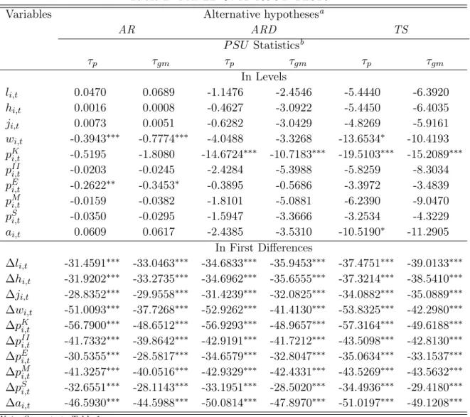
Table 2 presents the results for panel unit-roots tests for the cross-sectional variables
li,t,hi,t,ji,t,wi,t,pKi,t,pIIi,t,pEi,t,pi,tM,pSi,t andai,t. The test is first conducted in levels and
then in first differences.16 The table shows that for most variables, strong evidence of
I(1) behaviour exists, with somewhat less conclusive results for the relative price of capital pK
i,t.17
15See Gengenbach, Palm, and Urbain (2010) for a recent review of these methods. 16Not rejectingH
0in levels suggests that the variable is at leastI(1); rejectingH0in first difference suggests the variable is at mostI(1).
17We performed a Pesaran (2007) CIPS? test with an optimal lag length chosen with the Akaike
criterion to provide additional insight on the unit-root behaviour of the relative price of capital. The test results (not shown) show that evidence ofI(1)behaviour exists forpK
Table 2: Panel Unit-Root Tests
Variables Alternative hypothesesa
AR ARD TS P SU Statisticsb τp τgm τp τgm τp τgm In Levels li,t 0.0470 0.0689 -1.1476 -2.4546 -5.4440 -6.3920 hi,t 0.0016 0.0008 -0.4627 -3.0922 -5.4450 -6.4035 ji,t 0.0073 0.0051 -0.6282 -3.0429 -4.8269 -5.9161 wi,t -0.3943∗∗∗ -0.7774∗∗∗ -4.0488 -3.3268 -13.6534∗ -10.4193 pKi,t -0.5195 -1.8080 -14.6724∗∗∗ -10.7183∗∗∗ -19.5103∗∗∗ -15.2089∗∗∗ pII i,t -0.0203 -0.0245 -2.4284 -5.3988 -5.8259 -8.3034 pEi,t -0.2622∗∗ -0.3453∗ -0.3895 -0.5686 -3.3972 -3.4839 pMi,t -0.0159 -0.0382 -1.8101 -5.0881 -6.2390 -9.0470 pSi,t -0.0350 -0.0295 -1.5947 -3.3666 -3.2534 -4.3229 ai,t 0.0609 0.0617 -2.4385 -3.5310 -10.5190∗ -11.2905 In First Differences ∆li,t -31.4591∗∗∗ -33.0463∗∗∗ -34.6833∗∗∗ -35.9453∗∗∗ -37.4751∗∗∗ -39.0133∗∗∗ ∆hi,t -31.9202∗∗∗ -33.2735∗∗∗ -34.6962∗∗∗ -35.6555∗∗∗ -37.3214∗∗∗ -38.5410∗∗∗ ∆ji,t -28.8352∗∗∗ -29.9558∗∗∗ -31.4239∗∗∗ -32.0825∗∗∗ -34.0882∗∗∗ -35.0889∗∗∗ ∆wi,t -51.0093∗∗∗ -37.7268∗∗∗ -52.9262∗∗∗ -41.4130∗∗∗ -53.8325∗∗∗ -42.2980∗∗∗ ∆pKi,t -56.7900∗∗∗ -48.6512∗∗∗ -56.9293∗∗∗ -48.9657∗∗∗ -57.3164∗∗∗ -49.6188∗∗∗ ∆pIIi,t -41.7332∗∗∗ -39.8642∗∗∗ -42.9191∗∗∗ -41.7212∗∗∗ -43.5098∗∗∗ -42.8130∗∗∗ ∆pEi,t -30.5355∗∗∗ -28.5817∗∗∗ -34.6579∗∗∗ -32.8047∗∗∗ -35.0634∗∗∗ -33.1537∗∗∗ ∆pMi,t -41.3257∗∗∗ -40.0516∗∗∗ -42.9329∗∗∗ -42.4331∗∗∗ -43.5269∗∗∗ -43.5632∗∗∗ ∆pS i,t -32.6551∗∗∗ -28.1143∗∗∗ -33.1951∗∗∗ -28.5020∗∗∗ -34.4936∗∗∗ -29.4180∗∗∗ ∆ai,t -46.5930∗∗∗ -44.5988∗∗∗ -50.0814∗∗∗ -47.8970∗∗∗ -51.0197∗∗∗ -49.1208∗∗∗
Note: See note to Table 1.
aThe alternative hypotheses are an autoregressive model (AR), an autoregressive model with drift
(ARD) and a trend-stationary model (TS).
bWe resample the residuals vector 1000 times with a block bootstrap scheme with a block length
(B) equal to 1.75T1/3 to generate pseudodata with the null hypothesis of unit roots. The two test statistics are calculated for each bootstrap replication to get the approximated distribution of the statistics of interest.
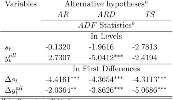
We complement this with Table 3, which provides the results of the augmented Dickey-Fuller (ADF) unit-root tests for the aggregate variables st and yallt , which are not
cross-sectional specific. The table reveals strong evidence of unit roots for these variables.18
hypotheses.
18Two other measures of the real effective exchange rate are discussed in Section 5.1. The ADF tests also indicate I(1)behaviour for these two measures.
Table 3: Unit-Root Tests for Aggregate Variables
Variables Alternative hypothesesa
AR ARD TS ADF Statisticsb In Levels st -0.1320 -1.9616 -2.7813 ytall 2.7307 -5.0412∗∗∗ -2.4194 In First Differences ∆st -4.4161∗∗∗ -4.3654∗∗∗ -4.3113∗∗∗ ∆yall t -2.0364∗∗ -3.8626∗∗∗ -5.0686∗∗∗
Note: See note to Table 1.
aThe alternative hypotheses are an autoregressive
model (AR), an autoregressive model with drift (ARD) and a trend-stationary model (TS).
bOptimal lag length chosen with the Akaike
crite-rion.
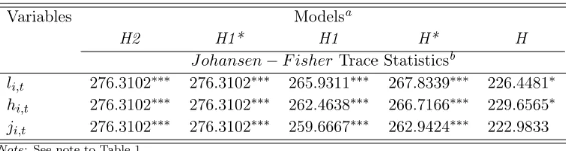
Cointegration Several panel cointegration tests have been suggested (McCoskey and Kao, 1998; Kao, 1999; Pedroni, 1999, 2001, 2004; Westerlund, 2005), which allow for various degrees of heterogeneity in the cointegrating coefficients. However, these tests are constructed so that the null and alternative hypotheses imply that all variables are either cointegrated or not cointegrated, with no allowance for the possibility that some variables are cointegrated and others are not. Moreover, it is often assumed that there exists at most one cointegrating relationship in the individual-specific models. System approaches to panel cointegration tests that do allow for more than one cointegrating relationship include the work of Larsson, Lyhagen, and Lothgren (2001) and Breitung (2005), who develop a likelihood-ratio test, and Maddala and Wu (1999), who use results in Fisher (1932) and propose an alternative approach to testing for cointegration in panel data by combining individual cross-sectional Johansen cointegration tests (Johansen, 1988, 1991) to obtain a test statistic for the full panel.
Recent contributions to the analysis of panel cointegration emphasize the importance of allowing for CSD, and the suggested solutions are similar to the panel unit-roots case.19 To obtain results that are robust to CSD of various forms, we implement the
Table 4: Panel Cointegration Tests
Variables Modelsa
H2 H1* H1 H* H
J ohansen−F isher Trace Statisticsb
li,t 276.3102∗∗∗ 276.3102∗∗∗ 265.9311∗∗∗ 267.8339∗∗∗ 226.4481∗
hi,t 276.3102∗∗∗ 276.3102∗∗∗ 262.4638∗∗∗ 266.7166∗∗∗ 229.6565∗
ji,t 276.3102∗∗∗ 276.3102∗∗∗ 259.6667∗∗∗ 262.9424∗∗∗ 222.9833
Note: See note to Table 1.
aThe models described the form of the deterministic components of the VEC(q) model
(see Johansen (1988, 1991)): no intercept or trend in the cointegrating relationships and no trend in the data (H2), intercepts in the cointegrating relationships and no trend in the data (H1*), intercepts in the cointegrating relationships and linear trends in the data (H1), intercepts and linear trends in the cointegrating relationships and linear trends in the data (H*), intercepts and linear trends in the cointegrating relationships and quadratic trends in the data (H).
bWe resample the residuals vector 1000 times with aniidbootstrap scheme to generate
pseudodata with the null hypothesis of no cointegration with an optimal lag order chosen by a Schwarz information criterion. The test statistics are calculated for each bootstrap replication to get the approximated distribution of the statistics of interest. The maximum eigenvalue test (not shown) was also calculated and yields the same conclusion.
Johansen-Fisher cointegration test (denoted λ), which is based on the combination of significance levels (p-value) of individual Johansen cointegration test statistics and has a χ2 distribution under the cross-sectional independence hypothesis.20 The presence
of CSD implies that the tests are not independent; hence, the λ-statistic does not have a χ2 distribution and must be approximated by bootstrap, as proposed in Maddala
and Wu (1999). We use the algorithm developed in Swensen (2006) for time series, and we extend it to the panel case. Table 4 presents the test results for the null hypothesis of no cointegration against the alternative of a non-zero cointegration rank. It reveals strong statistical evidence in favour of cointegration for our panel. Moreover, tests conducted over all the possible cointegration ranks (not shown) point to a rank between 1 and 3, depending on the model and specification. Our empirical analysis below thus accounts for multiple cointegrating vectors.
approaches applied to single cointegrating vector testing. 20If the test statistics are continuous, the significance levelsπ
i, fori= 1, . . . , N, are independent
uniform (0,1) variables, and −2 lnπi has a χ2 distribution with 2 degrees of freedom. Using the
additive property of theχ2variables, we get λ=−2PN
i=1lnπi andλhas aχ2distribution with 2N
Estimation Method Two popular techniques used to analyze a single-equation framework of cointegrated variables are the Fully Modified Ordinary Least Squares approach (Phillips and Hansen, 1990; Pedroni, 1996; Phillips and Moon, 1999) and the Dynamic Ordinary Least Squares approach (Saikkonen, 1991; Stock and Watson, 1993; Mark and Sul, 2003). Subsequent studies (Pedroni, 1996; Kao and Chiang, 1999; Phillips and Moon, 2000) show that these two techniques deliver unbiased estimators with standard normal distributions when applied to panel data. However, these estimators assume that explanatory variables are all I(1) but are not cointegrated.21
This drawback can be avoided by using system approaches.
System approaches to panel cointegration allowing for more than one cointegrating relationship include the work of Larsson et al. (2001), Groen and Kleibergen (2003) and Breitung (2005), who generalized the likelihood approach introduced in Pesaran et al. (1999). Breitung (2005) proposes a two-step estimation procedure that extends the Ahn and Reinsel (1990) and Engle and Yoo (1989) approach from the time series to the panel case. He considers a panel vector error-correction model set-up where only the cointegrating spaces are assumed to be identical for all cross-section members. In the first step of his procedure, the parameters (both long- and short-run) are estimated individually, and in the second step, the common cointegrating space is estimated in a pooled fashion. The resulting estimator is asymptotically efficient and normally distributed. Since results from Monte Carlo simulations in Breitung (2005) and Wagner and Hlouskova (2010) suggest that the two-step estimator has a good performance, we use this estimation method.22 Statistical inference is then based on
Driscoll-Kraay-Newey-West standard errors (Driscoll and Kraay, 1998).
We use a two-stage least-squares regression to estimate the industry-specific short-run
21If there is more than one cointegrating relationship, then the variance-covariance matrix of the residuals from the integrated process of the explanatory variables is singular and the results based on the asymptotic distribution is no longer valid.
22Even if there is more than one cointegrating relationship in the panel, we estimate only one relationship. This estimated relationship, in this case, still provides a consistent estimate of a cointegrating vector. Among the set of possible cointegrating relationships, the two-step estimator selects the relationship whose residuals are uncorrelated with any other I(1)linear combinations of the explanatory variables (Hamilton, 1994).
relationship to control for the potential endogeneity of wi,t. In the first stage, the
relative price of labour is regressed on all predetermined and exogenous variables in the model. The predicted values obtained from this regression are then used in the second stage.23
5
Results
This section presents our estimation results. First, Section 5.1 presents our estimates of the (long-term) cointegrating vector (3) and then Section 5.2 discusses the dynamic (error-correcting) adjustment process (5). Throughout, we report results obtained using all 20 manufacturing industries, as well as high- and low-NTE subsets of these industries. An extensive sensitivity analysis is provided, which explores the robustness of our results to alternative measures for the labour input, for the real effective exchange rate, for openness to trade, and for the price of intermediate inputs. In all tables of results, estimates superscripted by ∗, ∗∗ or ∗∗∗ indicate significance at the 10 percent, 5 percent and 1 percent levels, respectively.
5.1 Long-Term Effects (Cointegrating Vectors)
Benchmark Results Table 5 presents our benchmark estimates of the cointegrating vector in expression (3). Most estimates are highly statistically significant and are consistent with our theoretical priors. Notably, the own-price elasticity (the effect of
wi,t on labour input) is negative, while the impact of the price of capital (pKi,t) and that
of the price of intermediate inputs (pII
i,t) are positive, indicating substantial substitution
between labour and other inputs. As suggested by theory, the coefficient of the real effective exchange rate is negative, indicating that an appreciation of the Canadian dollar is associated with a decrease in manufacturing’s labour input,24 while the
23To facilitate the presentation of our results, the estimated industry-specific coefficients reported in the various tables (coefficients on time dummies reported in Tables 5 to 11 and all the coefficients in Tables 12 to 14) are the mean-group estimates, an aggregation of industry-specific estimated coefficients via an equally weighted linear combination. However, all the simulations are conducted using the industry-specific estimated coefficients, not the mean-group estimates.
24Since we estimate a linear model, the relationship is symmetric. A depreciation of the real exchange rate then yields an increase in manufacturing labour input. This symmetry applies to all
impact of world GDP (yall
t ) is positive. The enactment of the two trade agreements
has negative impacts on the labour input, a result compatible with earlier work (Gaston and Trefler, 1997; Beaulieu, 2000), indicating that trade liberalization has improved productivity but lowered employment in Canadian manufacturing industries. Finally, the transition towards a floating exchange rate regime is associated with a decrease in the labour input of manufacturing industries.
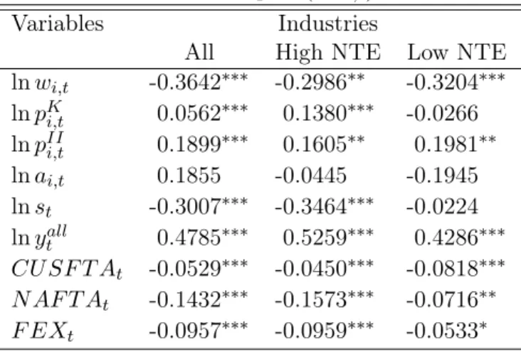
Table 5: Cointegrating Vectors
Labour Input (lnli,t)
Variables Industries
All High NTE Low NTE
lnwi,t -0.3642∗∗∗ -0.2986∗∗ -0.3204∗∗∗ lnpKi,t 0.0562∗∗∗ 0.1380∗∗∗ -0.0266 lnpIIi,t 0.1899∗∗∗ 0.1605∗∗ 0.1981∗∗ lnai,t 0.1855 -0.0445 -0.1945 lnst -0.3007∗∗∗ -0.3464∗∗∗ -0.0224 lnytall 0.4785∗∗∗ 0.5259∗∗∗ 0.4286∗∗∗ CU SF T At -0.0529∗∗∗ -0.0450∗∗∗ -0.0818∗∗∗ N AF T At -0.1432∗∗∗ -0.1573∗∗∗ -0.0716∗∗ F EXt -0.0957∗∗∗ -0.0959∗∗∗ -0.0533∗
Note: Estimates of the cointegrating vector of expression (3) in the text, using the methods described in Breitung (2005) and Pesaran et al. (1999). The three columns depict estimates obtained for all, high- and low-NTE industries. The symbols∗,∗∗and∗∗∗indicate statistical significance of the coefficient at the 10%, 5%and 1%
levels, respectively, using Driscoll-Kraay-Newey-West standard er-rors. Estimated coefficients and statistical inference forCU SF T At,
N AF T AtandF EXtare mean-group estimates.
The results in Table 5 are also economically significant. The estimate for the real exchange rate is -0.3007, indicating that a 10 percent real appreciation of the exchange rate is associated with a 3 percent long-term decrease in the labour input li,t. This
impact is stronger for high-NTE industries (0.3464, or a decrease of 3.5 percent following a 10 percent real appreciation), while it is negligible and not statistically significant for low-NTE industries.
The impact of the price of labour wi,t is also substantial and, at -0.3642, is estimated
to be of similar magnitude to that of the real exchange rate. The prices of other inputs (the price of capital pK
i,t and the price of intermediate inputspIIi,t) have positive impacts
of 0.0562 and 0.1899, respectively, suggesting that there is a substantial degree of substitution between labour and other inputs (see Appendix C for a discussion). The estimated impacts of wi,t and pIIi,t are of similar magnitude across industries, whereas
for the price of capital pK
i,t, the “all industries” average hides substantial differences
between industries open to trade (a strong positive effect) and for those that are not (a negligible and not statistically significant impact).
The impact of world GDP (yall
t ) is also important, with the benchmark estimate
suggesting a 0.48 percent long-run decrease in the labour input for each 1 percent decline in global demand for Canada’s manufactured products. The effect again varies across openness to trade and is larger for high-NTE industries. The two trade agreements have had statistically and economically significant impacts, with the enactment of NAFTA being associated with a 15 percent decrease in the labour input for high-NTE industries.25 Finally, Table 5 indicates that productivity has a
positive, but not statistically significant, impact on the labour input. According to the model described in Appendix C, this could suggest that Canadian manufacturing firms operate in environments with relatively low substitution across different goods.26 Overall, Table 5 shows that exchange rate movements have statistically and economi-cally significant long-run effects on the labour input of Canada’s manufacturing firms, with a 10 percent real appreciation being associated with a 3 percent decrease in the labour input. In addition, input prices, global demand, and trade agreements also have substantial effects, and an industry’s openness to trade is a key modifier to the magnitude of these impacts.
The impact of real exchange rate changes might be even stronger than suggested by the results in Table 5. If a real appreciation of the Canadian dollar makes imported
25The magnitude of the coefficient associated with NAFTA could, however, also signal the growing importance of China on the world manufacturing scene starting in the mid-1990s.
26An increase in productivity decreases marginal costs and, as a result, the price charged by the firm. The extent to which this price decrease results in a significant increase in demand – and a subsequent increase in labour demand – is governed by the elasticity of substitution across various products. If this elasticity is low, the coefficient on productivity could be negligible (see Appendix C).
capital more expensive and in turns leads to substitution away from capital and towards labour, an additional effect would be induced. However, the results in Table 5 suggest this added effect is likely to be small. Considering that across industries, roughly 1/6 of the capital input in our dataset is imported,27 and that the estimated
coefficient on the price of capital is relatively small (0.0562), the induced effect via imported capital (allowing for full pass-through of the appreciation into the Canadian price of imported capital28) would be−(0.0562)·1/6or around -0.01, a much smaller figure than the direct effect of -0.3007 in Table 5.
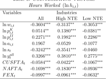
Sensitivity Analysis To study the robustness of our results, we first repeat our estimation of the cointegrating vectors using alternative measures of the labour input. In this context, Tables 6 and 7 below present results obtained using hours worked (hi,t) and jobs (ji,t), respectively, instead of the labour input (lit). Recall that hours
workedhi,t is a simple sum of hours worked with no control for skill and experience
(as is the case for lit), while ji,t is the total number of jobs, again with no allowance
for various work arrangements and experience differentials. Table 6: Cointegrating Vectors
Hours Worked (lnhi,t)
Variables Industries
All High NTE Low NTE
lnwi,t -0.3604∗∗∗ -0.3137∗∗ -0.3053∗∗∗ lnpKi,t 0.0514∗∗ 0.1380∗∗∗ -0.0381∗∗ lnpIIi,t 0.2271∗∗∗ 0.1982∗∗∗ 0.2286∗∗ lnai,t 0.1967 -0.0529 -0.1077 lnst -0.3242∗∗∗ -0.3541∗∗∗ -0.0460 lnytall 0.3266∗∗∗ 0.3810∗∗∗ 0.2775∗∗∗ CU SF T At -0.0584∗∗∗ -0.0422∗∗ -0.1067∗∗∗ N AF T At -0.1698∗∗∗ -0.1830∗∗∗ -0.0936∗∗∗ F EXt -0.0997∗∗∗ -0.0961∗∗∗ -0.0632∗
Note: See note to Table 5.
Significant differences between the benchmark results of Table 5 and those arrived at
27In KLEMS, capital is a composite of machinery and equipment, structures, inventories and land inputs. Of those, only machinery and equipment has a significant imported component. The average imported component for the capital composite is estimated at1/6 by Leung and Yuen (2005).
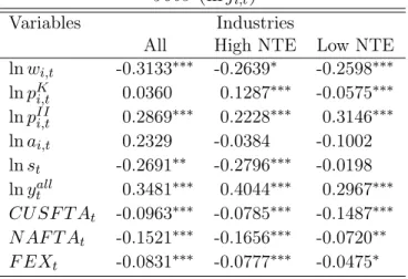
Table 7: Cointegrating Vectors
Jobs (lnji,t)
Variables Industries
All High NTE Low NTE
lnwi,t -0.3133∗∗∗ -0.2639∗ -0.2598∗∗∗ lnpK i,t 0.0360 0.1287∗∗∗ -0.0575∗∗∗ lnpIIi,t 0.2869∗∗∗ 0.2228∗∗∗ 0.3146∗∗∗ lnai,t 0.2329 -0.0384 -0.1002 lnst -0.2691∗∗ -0.2796∗∗∗ -0.0198 lnytall 0.3481∗∗∗ 0.4044∗∗∗ 0.2967∗∗∗ CU SF T At -0.0963∗∗∗ -0.0785∗∗∗ -0.1487∗∗∗ N AF T At -0.1521∗∗∗ -0.1656∗∗∗ -0.0720∗∗ F EXt -0.0831∗∗∗ -0.0777∗∗∗ -0.0475∗
Note: See note to Table 5.
using hours worked (Table 6) or jobs (Table 7) would suggest that changes to real exchange rates have compositional effects on the labour mix or on the organization of the workweek, in addition to the aggregate effects described above. Overall, however, the results are qualitatively similar across the three tables. One quantitative difference does emerge, in Table 7, where the estimated coefficients on the real exchange rate are shown to be substantially smaller for jobs than those arrived at with the other two definitions of the labour input: -0.2691 relative to -0.3007 in the benchmark for all industries and -0.2796 relative to -0.3464 for high-NTE industries. Such a result suggests that a given appreciation of the real value of the Canadian dollar is associated with a smaller long-run decrease in jobs than in hours worked, indicating that both intensive and extensive margins respond to exchange rate movements. By contrast, the estimated magnitude of the impact for CUSFTA is larger for jobs than it was for
li,t andhi,t. Notwithstanding these small differences, our results appear largely robust
to the definition of the labour input.
Next, Table 8 assesses the importance of our measure of trade openness. Recall that our benchmark results are based on the measure in Dion (2000), which controls for the importance of exports as a share of production and for imports as a share of the domestic market. By contrast, Table 8 uses data on Export Intensity (EI) only (from
Industry Canada) to classify industries into high- and low-EI.29 Table 8: Cointegrating Vectors
Export Intensity Variables Industries
All High EI Low EI
lnwi,t -0.3642∗∗∗ -0.1427 -0.4352∗∗∗ lnpKi,t 0.0562∗∗∗ 0.0882∗∗∗ 0.0786 lnpIIi,t 0.1899∗∗∗ -0.1742 0.3007∗∗∗ lnai,t 0.1855 -0.8884∗∗∗ 0.7227∗∗ lnst -0.3007∗∗∗ -0.4815∗∗∗ -0.0844 lnytall 0.4785∗∗∗ 0.8180∗∗∗ 0.1746∗ CU SF T At -0.0529∗∗∗ -0.0708∗∗∗ -0.0310∗ N AF T At -0.1432∗∗∗ -0.1455∗∗∗ -0.1142∗∗∗ F EXt -0.0957∗∗∗ -0.1088∗∗∗ -0.0646∗∗
Note: See note to Table 5.
This modification has important consequences for the magnitude and statistical sig-nificance of many estimates. First, the impact of the real exchange rate for industries highly open to trade is now -0.4815, 50 percent stronger than -0.3007, its “all indus-tries” counterpart (the coefficient for industries not open to trade remains low and not statistically significant). This suggests that it is for exporting industries, more than for industries affected by trade via imports, that appreciation and depreciation cycles in the real value of the Canadian dollar have important impacts. Similarly, the influence of worldwide product demand (the impact of yall
t ) is almost double in
industries highly open to trade, relative to their “all industries” benchmark. Overall, the results in Table 8 support benchmark estimates but single out exports as the key marker across which movements in the exchange rate and product demand affect the labour input of Canada’s manufacturers.
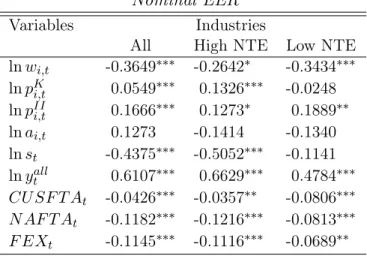
Continuing our robustness analysis, Tables 9 and 10 analyze alternative measures for the exchange rate. First, Table 9 presents results obtained using nominal effective exchange rates. Since movements in real exchange rates are often considered to be dominated by nominal rate changes (and only very gradual relative price adjustments),
29The first column of Table 8, for all industries, naturally reproduces the benchmark results of Table 5.
these might be sufficient to measure the actual ability of domestic producers to export abroad profitably. By contrast, Table 10 retains the idea of deflating nominal exchange rates, but uses relative unit labour costs (RULC) to do so. This deflating strategy follows a body of literature arguing that using unit labour costs to deflate exchange rates is a suitable method to accurately capture Canada’s ability to sell abroad profitably (Lafrance et al., 1998).
Table 9: Cointegrating Vectors
Nominal EER Variables Industries
All High NTE Low NTE
lnwi,t -0.3649∗∗∗ -0.2642∗ -0.3434∗∗∗ lnpKi,t 0.0549∗∗∗ 0.1326∗∗∗ -0.0248 lnpIIi,t 0.1666∗∗∗ 0.1273∗ 0.1889∗∗ lnai,t 0.1273 -0.1414 -0.1340 lnst -0.4375∗∗∗ -0.5052∗∗∗ -0.1141 lnytall 0.6107∗∗∗ 0.6629∗∗∗ 0.4784∗∗∗ CU SF T At -0.0426∗∗∗ -0.0357∗∗ -0.0806∗∗∗ N AF T At -0.1182∗∗∗ -0.1216∗∗∗ -0.0813∗∗∗ F EXt -0.1145∗∗∗ -0.1116∗∗∗ -0.0689∗∗
Note: See note to Table 5.
Alternative measures of exchange rates modify some of the quantitative results. No-tably, the estimated coefficients on exchange rates increase in magnitude when nominal effective exchange rates are used (Table 9), but this magnitude is then decreased when unit labour costs are used (Table 10). The pattern from Table 5, by which openness to trade increased this coefficient for high-NTE industries and reduced it to small, not statistically significant, numbers for low-NTE industries can also be seen in Tables 9 and 10. The impact of worldwide product demand (yallt ) similarly increases in Table 9 but is reduced in Table 10, relative to the benchmark results in Table 5.
Finally, Table 11 assesses a decomposition of the price of intermediate goods pIIi,t into the relative price of energy pE
i,t, of materials pMi,t and of services pSi,t. Interestingly,
this has the effect of reducing both the economic and statistical significance of the exchange rate. Since, at the same time, the price of energy is found to be both negative and very substantial economically, this result is probably explained by the
Table 10: Cointegrating Vectors
Real EER - RULC Variables Industries
All High NTE Low NTE
lnwi,t -0.3898∗∗∗ -0.3236∗∗∗ -0.3346∗∗∗ lnpK i,t 0.0752∗∗∗ 0.1524∗∗∗ -0.0055 lnpIIi,t 0.1238∗∗∗ 0.0256 0.1831∗∗ lnai,t 0.3972∗∗∗ 0.1945 -0.0717 lnst -0.1383∗∗∗ -0.1405∗ -0.0029 lnytall 0.1797∗∗∗ 0.2207∗∗∗ 0.2476∗∗∗ CU SF T At 0.0229∗∗ 0.0295∗∗ -0.0384∗ N AF T At -0.0699∗∗∗ -0.0771∗∗∗ -0.0470∗∗ F EXt -0.0316∗∗ -0.0378∗∗ -0.0166
Note: See note to Table 5.
high correlation between energy prices and the exchange rate of the Canadian dollar over the past two decades.
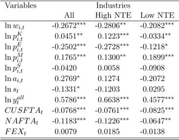
Table 11: Cointegrating Vectors
Disaggregated Prices of Intermediated Inputs Variables Industries
All High NTE Low NTE
lnwi,t -0.2672∗∗∗ -0.2806∗∗ -0.2082∗∗∗ lnpKi,t 0.0451∗∗ 0.1223∗∗∗ -0.0334∗∗ lnpEi,t -0.2502∗∗∗ -0.2728∗∗∗ -0.1218∗ lnpMi,t 0.1765∗∗∗ 0.1300∗∗ 0.1899∗∗∗ lnpS i,t -0.0420 0.0058 -0.0908 lnai,t 0.2769∗ 0.1274 -0.2072 lnst -0.1331∗ -0.1203 0.0295 lnytall 0.5786∗∗∗ 0.6638∗∗∗ 0.4577∗∗∗ CU SF T At -0.0768∗∗∗ -0.0761∗∗∗ -0.0825∗∗∗ N AF T At -0.1183∗∗∗ -0.1226∗∗∗ -0.0647∗∗ F EXt 0.0079 0.0185 -0.0138
Note: See note to Table 5.
In summary, our estimates of the cointegrating relationship (3) reveal important and robust findings: exchange rates and worldwide demand for Canadian products exert powerful long-run influences on the labour input of manufacturing firms, and these effects are stronger for industries that are more open to trade, particularly for exporters. Further, the enactment of two major trade agreements had an important negative effect on labour inputs. Finally, we find evidence that substantial levels of
substitution exist between labour and other inputs, so that increases in the price of capital and intermediary inputs lead to increases in the labour input of manufacturing firms. The next subsection explores the characteristics of the dynamic adjustment to these long-run properties.
5.2 Dynamic Adjustment (Error-Correcting Mechanism)
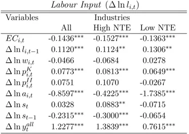
This subsection analyzes the adjustment towards the long-term cointegrating vector in (3). To this end, equation (5) is estimated via a two-stage least-squares framework that aims at correcting for possible problems of endogeneity between wages and the labour input. A general-to-specific strategy is used to establish the number of lags
p needed in (5), and the exchange rate is the only variable for which lagged values appear in a statistically significant manner. As a consequence, only the current values of wages, prices, productivity and world output appear in the three tables of results below, whereas for the exchange rate, both current and lagged values are present.30 Estimation results are provided in Tables 12-14 for the labour input, hours worked and jobs, respectively.
The first result of interest concerns the speed of adjustment towards the long-run labour input, governed by the estimate labeled ECi,t in the tables. Table 12 shows
that, in the benchmark case, this parameter equals −0.1436, indicating that about 15 percent of the gap between the targeted (frictionless) labour input and its actual value is closed every period-year. This 15 percent annual gap adjustment is fairly stable across industry types (high- or low-NTE) and for the alternative definitions of labour in Table 13 and Table 14. These results suggest the presence of significant costs of adjusting labour and a very gradual progression, with a half-life between 4
and 5 years, towards the target.
The second group of results of interest taken from Tables 12 to 14 concerns the influence of the exchange rate. As the tables indicate, the lagged values of the (growth in) exchange rates exert an important influence on the labour input of Canadian
Table 12: Short-term Dynamics
Labour Input (∆ lnli,t)
Variables Industries
All High NTE Low NTE
ECi,t -0.1436∗∗∗ -0.1527∗∗∗ -0.1363∗∗∗ ∆ lnli,t−1 0.1120∗∗∗ 0.1124∗∗ 0.1306∗∗ ∆ lnwi,t -0.0466 -0.0684 0.0278 ∆ lnpKi,t 0.0773∗∗∗ 0.0813∗∗∗ 0.0649∗∗∗ ∆ lnpIIi,t 0.0751 0.1070 -0.0267 ∆ lnai,t -0.8597∗∗∗ -0.4225∗∗∗ -1.7385∗∗∗ ∆ lnst 0.0328 0.0883∗∗ -0.0715 ∆ lnst−1 -0.2315∗∗∗ -0.3000∗∗∗ -0.0654 ∆ lnytall 1.2277∗∗∗ 1.3839∗∗∗ 0.7615∗∗∗ Note: Estimates of the short-term relationship (5) in the text. The three columns depict estimates obtained for all, high- and low-NTE industries. The symbols∗,∗∗ and ∗∗∗ indicate statistical signifi-cance of the coefficient at the10%,5%and1%levels, respectively. Estimated coefficients and statistical inference for all variables are mean-group estimates.
manufacturing firms.31 These results suggest that during the transition towards
its long-run target, the labour input of Canadian manufacturing firms is subjected to sizeable fluctuations associated with lagged movements in exchange rates. The numerical estimate suggests that, along this path, a 10 percent appreciation of the Canadian currency would cause (ultimately transitory) decreases in the labour input by a factor of between 2 percent and 2.5 percent. Decomposing industries into high-and low-NTE shows that this effect is particularly present for high-NTE industries high-and not statistically significant for low-NTE ones. It is interesting to note that only the lagged values of∆st have a statistically significant impact: exchange rate movements
appear to have only a lagged protracted impact on the labour input. Table 14 also shows that the exchange rate affects both the intensive and the extensive margins: industries tend to decrease not only the total number of jobs, but also the average number of hours worked for remaining jobs.
Third, the tables reveal that multifactor productivity ai,t also affects the dynamic
adjustment trajectory. Specifically, Tables 12 to 14 reveal that a 1 percent increase
31Recall that this effect is separate from the one arising when thelevel of the exchange rate affects the long-run (frictionless) labour input.
Table 13: Short-term Dynamics
Hours Worked (∆ lnhi,t)
Variables Industries
All High NTE Low NTE
ECi,t -0.1276∗∗∗ -0.1349∗∗∗ -0.1338∗∗∗ ∆ lnli,t−1 0.1160∗∗∗ 0.1219∗∗∗ 0.1304∗∗ ∆ lnwi,t -0.0576 -0.0743 0.0213 ∆ lnpKi,t 0.0735∗∗∗ 0.0810∗∗∗ 0.0553∗∗∗ ∆ lnpIIi,t 0.0597 0.0926 -0.0582 ∆ lnai,t -0.8554∗∗∗ -0.4308∗∗∗ -1.6960∗∗∗ ∆ lnst 0.0219 0.0643 -0.0633 ∆ lnst−1 -0.2445∗∗∗ -0.3105∗∗∗ -0.0791 ∆ lnytall 1.2606∗∗∗ 1.4110∗∗∗ 0.7954∗∗∗ Note: See note to Table 12.
Table 14: Short-term Dynamics
Jobs (∆ lnji,t)
Variables Industries
All High NTE Low NTE
ECi,t -0.1265∗∗∗ -0.1241∗∗∗ -0.1664∗∗∗ ∆ lnli,t−1 0.1949∗∗∗ 0.2013∗∗∗ 0.2048∗∗∗ ∆ lnwi,t -0.0945∗∗ -0.1448∗∗∗ 0.0522 ∆ lnpKi,t 0.0503∗∗∗ 0.0538∗∗∗ 0.0399∗∗ ∆ lnpIIi,t 0.0635 0.1086 -0.0735 ∆ lnai,t -0.5864∗∗∗ -0.1958∗∗ -1.3108∗∗∗ ∆ lnst 0.0123 0.0603 -0.0817 ∆ lnst−1 -0.2096∗∗∗ -0.2627∗∗∗ -0.0788 ∆ lnytall 1.1357∗∗∗ 1.3098∗∗∗ 0.6142∗∗∗ Note: See note to Table 12.
in productivity reduces labour by close to 1 percent (0.86) for the measures of labour and hours worked (Tables 12 and 13) but by less for jobs (Table 14). Recall that multifactor productivity was found to have a positive, but not statistically significant, influence on the long-run labour input. Its impact on the short-term labour input may suggest institutional aspects that make it hard for firms to quickly expand production when productivity increases and lead them to service the same markets with a reduced labour input. Finally, Tables 12 to 14 show that world output also has an important effect on the dynamic adjustment towards the long-run equilibrium, in addition to the impact it had on the long-run level. The tables reveal that this impact is large,
more than one for one, and is especially important for high-NTE industries.
Figure 2 provides a useful way to visualize the value added of the dynamic adjustment component of our estimation strategy. Panel (a) of the figure plots observed values for labour against the value predicted by the long-run relationship (3) only, without allowing for the dynamic adjustment (5), while Panel (b) depicts the observed and predicted series according to the full model (5), which accounts for both the estimated long-run relationship and the dynamic adjustment towards that long-run relationship. The figure shows that the full model, which includes the dynamic adjustment com-ponents, is better able to fit both the levels and the timing of the swings in labour input over our sample.32
6
Conclusion
We present evidence that the boom-bust cycles experienced in the labour market of Canada’s manufacturing industries over the past five decades are strongly connected to fluctuations in the exchange rate of the Canadian dollar. Our econometric strategy employs panel data estimation techniques and carefully controls for the unit root, cointegration and cross-sectional dependence found in the data. Our results suggest that a 10 percent appreciation of the Canadian dollar can decrease hours worked and jobs by around 3 percent and that this effect occurs relatively slowly, with about 15 percent of the gap between the actual and targeted labour input being closed every year. These results are significantly stronger in industries with above-average net trade exposure. We also provide evidence that the enactment of two major trade agreements in 1989 and 1994 had sizeable negative impacts on the number of hours worked and the number of jobs in Canadian manufacturing industries. These results are timely, as the more recent period of depreciation of the currency has led to conjectures about
32The figure plots the observed and predicted values of the labour input in the all-industries case. Predicted labour is generated recursively by the model for each year, with the initial year in our sample (1961) serving as the initial condition. This recursive method implies that the actual lagged labour input is never used to generate the predictions. The root-mean-square error is reduced by close to 28 percent by using the full model.
2900 3100 3300 3500 3700 3900 4100 4300 1961 1964 1967 1970 1973 1976 1979 1982 1985 1988 1991 1994 1997 2000 2003 2006 Observed
Predicted (Cointegrating Relationship)
(a) 2900 3100 3300 3500 3700 3900 4100 4300 1961 1964 1967 1970 1973 1976 1979 1982 1985 1988 1991 1994 1997 2000 2003 2006 Observed
Predicted (Error-Correction Model)
(b)
Figure 2: Hours Worked Dynamic In-Sample Predictions for (a) Cointegrating (Long-run) Relationship only and for (b) Error-correction Model
whether manufacturing in Canada will rebound.
References
Ahn, S. K. and G. C. Reinsel(1990): “Estimation for Partially Nonstationary
Mul-tivariate Autoregressive Models,” Journal of the American Statistical Association, 85, pp. 813–823.
Bai, J. and S. Ng (2004): “A PANIC Attack on Unit Roots and Cointegration,” Econometrica, 72, 1127–1177.
Baltagi, B. H. and C. Kao(2000): “Nonstationary Panels, Cointegration in Panels
and Dynamic Panels: A Survey,” Center for Policy Research Working Papers 16, Center for Policy Research, Maxwell School, Syracuse University.
Banerjee, A., M. Marcellino, and C. Osbat (2004): “Some cautions on the
use of panel methods for integrated series of macroeconomic data,” Econometrics Journal, 7, 322–340.
Beaulieu, E. (2000): “The Canada-US Free Trade Agreement and labour market
adjustment in Canada,” Canadian Journal of Economics, 33, 540–563.
Breitung, J. (2005): “A Parametric approach to the Estimation of Cointegration
Vectors in Panel Data,” Econometric Reviews, 24, 151–173.
Bruneau, G. and K. Moran (2012): “Exchange Rate Fluctuations and Labour
Market Adjustments inCanadian Manufacturing Industries,” Working Paper 12-27, CIRPEE.
Burgess, S. M. and M. M. Knetter (1998): “An international comparison of
employment adjustment to exchange rate fluctuations,” Review of International Economics, 6, 151–63.
Campa, J. M. and L. S. Goldberg(2001): “Employment versus wage adjustment
Cerrato, M. and N. Sarantis (2007): “A bootstrap panel unit root test under cross-sectional dependence, with an application toPPP,” Computational Statistics & Data Analysis, 51, 4028 – 4037.
Chang, Y. (2004): “Bootstrap unit root tests in panels with cross-sectional
depen-dency,” Journal of Econometrics, 120, 263–293.
Choi, I.(2001): “Unit root tests for panel data,” Journal of International Money and Finance, 20, 249–272.
——— (2002): “Combination Unit Root Tests for Cross-Sectionally Correlated Panels,” Working papers, Hong Kong University of Science and Technology.
Dekle, R. (1998): “The yen and Japanese manufacturing employment,” Journal of International Money and Finance, 17, 785–801.
Di Iorio, F. and S. Fachin (2009): “A residual-based bootstrap test for panel
cointegration,” Economics Bulletin, 29, 3222–3232.
Dion, R. (2000): “Trends in Canada’s merchandise trade,” Bank of Canada Review,
Winter, 29–41.
Driscoll, J. C. and A. C. Kraay(1998): “Consistent covariance matrix estimation
with spatially dependent panel data,” The Review of Economics and Statistics, 80, 549–560.
Eberhardt, M. and F. Teal (2011): “Econometrics For Grumblers: A New Look
At The Literature On Cross-Country Growth Empirics,” Journal of Economic Surveys, 25, 109–155.
Engle, R. and B. Yoo (1989): “Cointegrated Economic Time Series: A Survey
With New Results,” Papers 8-89-13, Pennsylvania State - Department of Economics.
Fachin, S. (2007): “Long-run trends in internal migrations in Italy: a study in panel
Fisher, R. A. (1932): Statistical Methods for Research Workers, Edinburgh: Oliver & Boyd, 4th ed.
Gaston, N. and D. Trefler (1997): “The labour market consequences of the
Canada-U.S. Free Trade Agreement,” Canadian Journal of Economics, 30, 18–41.
Gengenbach, C., F. Palm, and J.-P. Urbain (2010): “Panel Unit Root Tests
in the Presence of Cross-Sectional Dependencies: Comparison and Implications for Modelling,” Econometric Reviews, 29, 111–145.
Groen, J. J. J. and F. Kleibergen (2003): “Likelihood-Based Cointegration Analysis in Panels of Vector Error-Correction Models,” Journal of Business & Economic Statistics, 21, 295–318.
Hadri, K. (2000): “Testing for stationarity in heterogeneous panel data,” Economet-rics Journal, 3, 148–161.
Hamermesh, D. S. and G. A. Pfann (1996): “Adjustment costs in factor demand,” Journal of Economic Literature, 34, 1264–1292.
Hamilton, J. D. (1994): Time Series Analysis, Princeton University Press.
Hansen, B. E. (1997): “Approximate Asymptotic P Values for Structural-Change
Tests,” Journal of Business & Economic Statistics, 15, 60–67.
Harris, R. D. F. and E. Tzavalis (1999): “Inference for unit roots in dynamic
panels where the time dimension is fixed,” Journal of Econometrics, 91, 201–226.
Im, K. S., M. H. Pesaran, and Y. Shin (2003): “Testing for unit roots in
hetero-geneous panels,” Journal of Econometrics, 115, 53–74.
Issa, R., R. Lafrance, and J. Murray (2008): “The turning black tide: energy
prices and the Canadian dollar,” Canadian Journal of Economics, 41, 737–759.
Johansen, S. (1988): “Statistical analysis of cointegration vectors,” Journal of Economic Dynamics and Control, 12, 231–254.