Statistical Analysis of Network Data

(1)

Statistical Analysis of Network Data

A Brief Overview

Eric D. Kolaczyk

Dept of Mathematics and Statistics, Boston University

(2)

Focus of this Talk

In this talk I will present a brief overview of the foundations common to the statistical analysis of network data across the disciplines, from a statistical perspective.

Approach will be that of a high-level, whirlwind overview of the topics of network summary and visualization

network sampling

network modeling and inference, and network processes.

Concepts will be illustrated drawing on examples from bioinformatics, computer network traffic analysis, neuroscience, and social networks.

(3)

Resources

Organization and presentation of material in this quick talk will largely parallel that in

1

USE R ! Use R ! Use R ! Eric Kolaczyk Gábor Csárdi

Statistical

Analysis of

Network Data

with R

Sta

tistical Analysis of Net

w ork Da ta with R Kolacz yk · Csár di

Eric Kolaczyk · Gábor Csárdi Statistical Analysis of Network Data with R

Th is book is the fi rst of its kind in network research. It can be used as a stand-alone resource in which multiple R packages are used to illustrate how to use the base code for many tasks. igraph is the central package and has created a standard for developing and manipulating network graphs in R. Measurement and analysis are integral components of network research. As a result, there is a critical need for all sorts of statistics for network analysis, ranging from applications to methodology and theory. Networks have permeated everyday life through everyday realities like the Internet, social networks, and viral marketing, and as such, network analysis is an important growth area in the quantitative sciences. Th eir roots are in social network analysis going back to the 1930s and graph theory going back centuries. Th is text also builds on Eric Kolaczyk’s book Statistical Analysis of Network Data (Springer, 2009).

Eric Kolaczyk is a professor of statistics, and Director of the Program in Statistics, in the Department of Mathematics and Statistics at Boston University, where he also is an affi liated faculty member in the Bioinformatics Program, the Division of Systems Engineering, and the Program in Computational Neuroscience. His publications on network-based topics, beyond the development of statistical methodology and theory, include work on applications ranging from the detection of anomalous traffi c patterns in computer networks to the prediction of biological function in networks of interacting proteins to the characterization of infl uence of groups of actors in social networks. He is an elected fellow of the American Statistical Association (ASA) and an elected senior member of the Institute of Electrical and Electronics Engineers (IEEE).

Gábor Csárdi is a research associate at the Department of Statistics at Harvard University, Cambridge, Mass. He holds a PhD in Computer Science from Eötvös University, Hungary. His research includes applications of network analysis in biology and social sciences, bioinformatics and computational biology, and graph algorithms. He created the igraph soft ware package in 2005 and has been one of the lead developers since then.

(4)

Our Focus

. . .

The statistical analysis ofnetwork data

i.e., analysis of measurements either ofor froma system conceptualized as a network.

Challenges:

relational aspect to the data;

complex statistical dependencies (often the focus!); high-dimensional and often massive in quantity.

(5)

Outline

1 Introduction 2 Network Mapping 3 Network Characterization 4 _{Network Sampling} 5 Network Modeling 6 Network Inference

(6)

Descriptive Statistics for Networks

First two topics go together naturally, i.e., network mapping

characterization of network graphs

May seem ‘soft’ . . . but it’s important!

This is basically descriptive statistics for networks.

Probably constitutes at least 2/3 of the work done in this area.

Note: It’s sufficiently different from standard descriptive statistics that it’s something unto itself.

(7)

Network Mapping

What is ‘network mapping’ ?

Production of a network-based visualization of a complex system.

What is ‘the’ network?

Network as a ‘system’ of interest;

Network as a graph representing the system; Network as a visual object.

(8)

Example: Mapping Belgium Which of these is ‘the’ Belgium?

(9)

(10)

Outline

1 Introduction 2 Network Mapping 3 Network Characterization 4 _{Network Sampling} 5 Network Modeling 6 Network Inference 7 Wrap-Up

(11)

Characterization of Network Graphs: Intro

Given a network graph representation of a system (i.e., perhaps a result of

network mapping), often questions of interestcan be phrased in terms of

structural propertiesof the graph.

social dynamics can be connected topatterns of edges among vertex

triples;

routes for movement of informationcan be approximated by shortest

paths between vertices;

‘importance’ of vertices can be captured through so-calledcentrality

measures;

(12)

Characterization Intro (cont.)

Structural analysis of network graphs ≈descriptive analysis; this is a

standard first (and sometimes only!) step in statistical analysis of networks.

Main contributors of tools are social network analysis,

mathematics & computer science, statistical physics

Many tools out there . . . two rough classes include

characterization of vertices/edges, and characterization of network cohesion.

(13)

Characterization of Vertices/Edges

Examples include Degree distribution Vertex/edge centrality Role/positional analysis

(14)

Centrality: Motivation

Many questions related to ‘importance’ of vertices. Which actors hold the ‘reins of power’ ?

How authoritative is a WWW page considered by peers? The deletions of which genes is more likely to be lethal? How critical to traffic flow is a given Internet router?

Researchers have sought to capture the notion of vertex importance through so-called centrality measures.

(15)

Centrality: An Illustration

Clockwise from top left: (i) toy graph, with (ii) closeness, (iii) between-ness, and (iv) eigenvector centralities.

Example and figures

courtesy of Ulrik Bran-des.

(16)

Network Cohesion: Motivation

Many questions involve scales coarser than just individual vertices/edges. More properly considered questions regarding ‘cohesion’ of network.

Do friends of actors tend to be friends themselves? Which proteins are most similar to each other?

Does the WWW tend to separate according to page content? What proportion of the Internet is constituted by the ‘backbone’ ?

(17)

Network Cohesion: Various Notions!

Various notions of ‘cohesion’. density clustering connectivity flow partitioning . . . and more. . .

(18)

Illustration: Detecting Malicious Internet Sources

Ding et al.a use the idea of

cut-vertices to detect Internet IP

addresses associated with malicious behavior.

Corresponds to a type of (anti)social behavior.

a

Ding, Q., Katenka, N., Barford, P., Kolaczyk, E.D., and Crovella, M. (2012). Intrusion as (Anti)social Communication:

Characterization and Detection.Proceedings of

the 2012 ACM SIGKDD Conference on Knowledge Discovery and Data Mining.

Source/Destination Network

(19)

Outline

(20)

Network Sampling: Point of Departure

. . .

Common modus operandiin network analysis:

System of elements and their interactions is of interest. Collect elements and relations among elements.

Represent the collected data via a network. Characterize properties of the network.

(21)

Interpretation: Two Scenarios

With respect to what frame of reference are the network characteristics interpreted?

1 The collected network data are themselves the primary object of

interest.

2 The collected network data are interesting primarily as representative

of an underlying ‘true’ network.

The distinction is important!

(22)

Common Network Sampling Designs

Viewed from the perspective of classical statistical sampling theory, the network sampling design is important.

Examples include

Induced Subgraph Sampling Incident Subgraph Sampling Snowball Sampling

(23)

Common Network Sampling Designs (cont.)

Induced Subgraph Sampling Incident Subgraph Sampling

s1

(24)

Caveat emptor

. . .

Completely ignoring sampling issues is equivalent to using ‘plug-in’ estimators.

The resulting bias(es) can be both substantial and unpredictable!

BA PPI AS arXiv

Degree Exponent ↑ ↑ ↓ ↑ ↑ = = = ↓ ↑ ↑ ↓

Average Path Length ↑ ↑ = ↑ ↑ ↓ ↑ ↑ ↓ ↑ ↑ ↓

Betweenness ↑ ↑ ↓ ↑ ↑ ↓ ↑ ↑ ↓ = = =

Assortativity = = ↓ = = ↓ = = ↓ = = ↓

Clustering Coefficient = = ↑ ↑ ↓ ↑ ↓ ↓ ↑ ↓ ↓ ↓

Lee et al (2006): Entries indicate direction of bias for induced subgraph

(25)

Accounting for Sampling Design

Accounting for sampling design can be non-trivial.

Classical work goes back to the 1970’s (at least), with contributions of Frank and colleagues, based mainly on Horvitz-Thompson theory. More recent resurgence of interest, across communities, has led to additional studies using both classical and modern tools.

(26)

Illustration: Estimation of Degree Distribution

Under a variety of sampling designs, the following holds:

E[N∗] =PN , (1)

where

N= (N0,N1, ...,NM): the true degree vector, for

Ni: the number of vertices with degreei in the original graph

N∗ = (N₀∗,N₁∗, ...,N_M∗): the observed degree vector, for

N_i∗: the number of vertices with degree i in the sampled graph

P is an M+ 1 byM+ 1 matrix operator, where

(27)

Estimating Degree Distribution: An Inverse Problem

Ove Frank (1978) proposed solving for the degree distribution by an

unbiased estimator ofN, defined as

ˆ

Nnaive=P−1N∗ . (2)

There are two problems with this simple solution:

1 The matrix P is typically not invertible in practice.

(28)

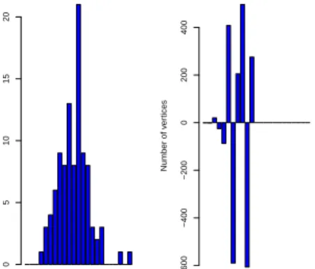
Does It Really Matter? Yes!

0 3 6 9 13 17 21

True Degree Sequence

Degree Number of v er tices 0 5 10 15 20 0 3 6 9 13 17 21 Naive Estimated Degree Sequence Degree Number of v er tices −600 −400 −200 0 200 400

Figure : Left: ER graph with 100 vertices and 500 edges. Right: Naive estimate of degree distribution, according to equation (2). Data drawn according to

(29)

A Modern Variant: Constrained, Penalized WLS

We have recently proposed1 a penalized weighted least squares with

additional constraints. minimize N (PN−N ∗₎T C−1(PN−N∗) +λ·pen(N) subject to Ni ≥0, i = 0,1, . . .M M X i=0 Ni =nv , (3) where C = Cov(N∗),

pen(N) is a penalty on the complexity of N,

(30)

Application to Online Social Networks

0 5 10 −15 −10 −5 log2(degree) log2(freq) Friendster cmty 1−5 0 5 10 −15 −10 −5 log2(degree) log2(freq) Friendster cmty 6−15 0 5 10 −15 −10 −5 log2(degree) log2(freq) Friendster cmty 16−30 0 5 10 −15 −10 −5 log2(degree) log2(freq) Orkut cmty 1−5 0 5 10 −15 −10 −5 log2(degree) log2(freq) Orkut cmty 6−15 0 5 10 −15 −10 −5 log2(degree) log2(freq) Orkut cmty 16−30 0 5 10 −15 −10 −5 log2(degree) log2(freq) LiveJournal cmty 1−5 0 5 10 −15 −10 −5 log2(degree) log2(freq) LiveJournal cmty 6−15 0 5 10 −15 −10 −5 log2(degree) log2(freq) LiveJournal cmty 16−30 Figure :

(31)

Estimating Approximate Epidemic Thresholds: Friendster

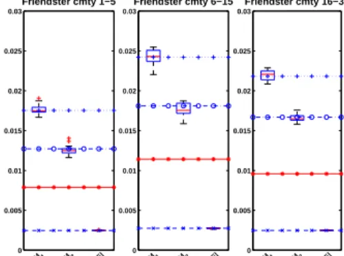
Moments of degree distributions can be used to obtain bounds of the network’s epidemic

thresholdτc.

An approximate threshold is give by the inverse of the largest

eigenvalueλ1 of the adjacency

matrix (Mieghem, Omic, & Kooij ’09).

Simple bounds forλ1 are

0 0.005 0.01 0.015 0.02 0.025 0.03 Friendster cmty 1−5 1 / M 1 1/ √ M2 1 / √ |E| 0 0.005 0.01 0.015 0.02 0.025 0.03 Friendster cmty 6−15 1 / M 1 1/ √ M2 1 / √ |E| 0 0.005 0.01 0.015 0.02 0.025 0.03 Friendster cmty 16−30 1 / M 1 1/ √ M2 1 / √ |E|

(32)

Outline

(33)

Two Scenarios

We will look at two complementary scenarios2:

1 we observe a network G (and possibly attributesX) and we wish to

model G (and X);

2 we observe the networkG, but lack some or all of the attributes X,

and we wish to inferX.

(34)

High Standards

Statisticians demand a great deal of their modeling:

1 theoretically plausible

2 estimable from data

3 _{computationally feasible estimation strategies}

4 quantification of uncertainty in estimates (e.g., confidence intervals)

5 _{assessment of goodness-of-fit}

6 understanding of the statistical properties of the overall procedure

(35)

Classes of Statistical Network Models

Roughly speaking, there are network-based versions of three canonical classes of statistical models:

1 regression models (i.e., ERGMs)

2 latent variable models (i.e., latent network models)

(36)

Statistical Network Models: Progress and Challenges

This is one of the most active areas of research in statistics and networks. Most work in ERGMs and SBMs.

A few high-level comments:

ERGMS have the largest body of work associated with them . . . . . . but they also arguably have the greatest number of problems (i.e., degeneracy, instability, problems under sampling, as well as the least supporting formal theory).

SBMs arguably have the most extensive theoretical development (i.e., fully general formulation, consistency and asymptotic normality of parameter estimates, etc.) . . .

(37)

Processes on Network Graphs

So far we have focused on network graphs, as representations of network

systems of elements and their interactions.

But often it is some quantity associated with the elements that is of most

interest, rather than the network per se.

Nevertheless, such quantities may be influenced by the interactions among

elements. Examples:

Behaviors and beliefs influenced by social interactions.

(38)

Illustration: Predicting Signaling in Yeast

● ● ● ● ● ● ●● ● ● ● ● ● ● ● ● ● ● ● ● ● ● ● ● ● ● ● ● ● ● ● ● ● ● ● ●● ● ● ● ● ● ● ● ● ● ● ● ● ● ● ● ● ● ● ● ● ● ● ● ● ● ● ● ● ● ● ● ● ● ● ● ● ● ● ● ● ● ● ● ● ● ● ● ● ● ● ● ● ● ● ● ● ● ● ● ● ● ● ● ● ● ● ● ● ● ● ● ● ● ● ● ● ● ● ● ● ● ● ● ● ● ● ● ● ● ● ● ● ● ● ● ● ●

Baker’s yeast (i.e., S.

cerevisiae)

All proteins known to

participate incell

communicationand their

interactions

Question: Is knowledge of

the function of a protein’s neighbors predictive of that protein’s function?

(39)

A Simple Approach: Nearest-Neighbor Prediction

Egos w/ ICSC

Proportion Neighbors w/ ICSC

Frequency 0.0 0.2 0.4 0.6 0.8 1.0 0 5 15 25

Egos w/out ICSC

Frequency 0.0 0.2 0.4 0.6 0.8 1.0 0 5 15 25

A simple predictive algorithm uses nearest neighbor princi-ples. Let Xi = ( 1,if corporate 0,if litigation Compare P j∈Nixj

(40)

Modeling Static Network-Indexed Processes

The nearest-neighbor algorithm (also sometimes called

‘guilt-by-association’), although seemingly informal, can be quite competitive with more formal, model-based methods.

Various models have been proposed for static network-indexed processes. Two commonly used classes/paradigms:

Markov random field (MRF) models

=⇒ Extends ideas from spatial/lattice modeling.

Kernel-learning regression models

(41)

Outline

(42)

Network Topology Inference

Recall our characterization ofnetwork mapping, as a three-stage process

involving

1 Collecting relational data

2 _{Constructing a network graph representation}

3 _{Producing a visualization of that graph}

Network topology inference is the formalization of Step 2 as a task in statistical inference.

Note: Casting the task this way also allows us to formalize the question of validation.

(43)

Network Topology Inference (cont.)

There are many variants of this problem!

Three general, and fairly broadly applicable, versions are Link prediction

Association network inference Tomographic network inference

(44)

Schematic Comparison of Inference Problems

Original Network Link Prediction

(45)

Link Prediction: Examples

● ● ● ● ● ● ● ● ● ● ● ● ● ● ● ● ● ● ● ● ● ● ● ● ● ● ● ● ● ● ● ● ● ● ● ● ● ● ● ● ● ● ● ● ● ● ● ● ● ● ● ● ● ● ● ● ● ● ● ● ● ● ● ● ● ● ● ● ● ● ● ● ● ● ● ● ● ● ● ● ● ● ● ● ● ● ● ● ● ● ● ● ● ● ● ● ● ● ● ● ● ● ● ● ● ● ● ● ● ● ● ● ● ● ● ● ● ● ● ● ● ● ● ● ● ● ● ● ● ● ● ● ● ● ● ● ● ● ● ● ● ● ● ● ● ● ● ● ● ● ● ● ● ● ● ● ● ● ● ● ● ● ● ● ● ● ● ● ● ● ● ● ● ● ● ● ● ● ● ● ● ● ● ● ● ● ● ● ●

Examples of link prediction in-clude

predicting new hyperlinks in the WWW

assessing the reliability of declared protein

interactions

predicting international relations between countries

(46)

Link Prediction: Problem & Solutions

Goal is to predict the edge

sta-tus’ Ymiss for all potential edges

with missing (i.e., unknown) sta-tus, based on

observed status’Yobs, and

any other auxilliary information.

Two main classes of methods pro-posed in the literature to date.

Scoring methods Classification methods See Kolaczyk (2009), Chapter 7.2.

(47)

Link Prediction: Illustration

0 5 10 15 20 25 30 35 No Edge Edge ● ●

Number of Common Neighbors

Scoring methods come in all

shapes and sizes.

Number of common neighbors a basic example.

Sufficient here (in a network of blogs) to obtain substantial

dis-crimination (e.g., AUC of ∼0.9

(48)

Outline

(49)

Wrapping Up

Lots of additional topics we have not touched upon: Dynamic networks

Weighted networks Community detection Etc.

(50)

Wrapping Up (cont.)

Some of the things my group is working on currently include: Uncertainty in graph summary statistics under noisy conditions. Asymptotics for parameter estimation in network models. Estimation of degree distributions from sampled data. Bayesian latent-factor network perturbation models. Multi-attribute networks.