Bank Risk: Does Size Matter?

Edith Cowan University Edith Cowan University

Research Online

Research Online

ECU Publications 2011

1-1-2011

Bank Risk: Does Size Matter?

Bank Risk: Does Size Matter?

Edith Cowan University

Akhmad R. Kramadibrata

Edith Cowan University

Robert Powell

Edith Cowan University

Abhay K. Singh

Edith Cowan University

Follow this and additional works at: https://ro.ecu.edu.au/ecuworks2011 Part of the Finance Commons

This is an Author's Accepted Manuscript of: Allen, D. E., Kramadibrata, A. R., Powell, R.J. , & Singh, A.K. (2011). Bank risk: does size matter?. Paper presented at the 2011 Australasian Meetings of the Econometric Society. Adelaide, Australia. Available here

The copyright to this article is held by the Econometric Society, http://www.econometricsociety.org/. It may be downloaded, printed and reproduced only for personal or classroom use. Absolutely no downloading or copying

Bank Risk: Does Size Matter?

David E. Allen Akhmad R. Kramadibrata

Robert J. Powell1 Abhay K. Singh

Edith Cowan University

Abstract

The size of banks is examined as a determinant of bank risk. A wide range of banks are examined across four regions, including Australia, Canada, Europe and the USA. Four risk metrics are considered including Value at Risk (VaR), Conditional Value at Risk (CVaR, which measures risk beyond VaR), Probability of Default (PD) using Merton structural methodology, and Conditional Probability of Default (CPD, the author’s own model which measures risk based on extreme asset value fluctuations. Daily equity and asset value fluctuations are included in the analysis, including pre-GFC and pre-GFC periods. In addition to examining size in isolation as a determinant of bank risk, the paper uses fixed effects panel data regression to examine the significance of size as a risk determinant in conjunction with a range of other independent variables. The study finds mixed results among the four regions with no conclusive evidence of significant association between size and risk.

Keywords

Bank Risk, Value at Risk; Conditional Value at Risk; Probability of Default; Conditional Probability of Default.

JEL Codes

G01, G21, G28

Acknowledgements: We are thankful to the Australian Research Council and Edith Cowan University for funding support.

1 _{Corresponding Author: Robert Powell, School of Accounting, Finance and Economics, Edith Cowan}

1. Introduction

The question addressed is whether there is association between the size of a bank and its risk. Prior studies have mixed findings as to determinants of bank risk (using risk measures such as share price volatility and default), with independent variables including a variety of balance sheet and profitability items. Several studies consider diversification of bank income sources as a determinant of bank risk (for example, Acharya, Hasan, & Saunders, 2006; Cornett, Ors, & Tehranian, 2002; De Young & Roland, 2001; Saunders & Walter, 1994; Stiroh, 2004; Stiroh, 2006; Stiroh & Rumble, 2006). Other studies find that balance sheet and income statement items or ratios provide little explanation of bank risk, and that changes in volatility and default are often caused by external shocks or contagion. Several studies have considered the contagion aspect (for example, Das, Duffie, Kapadia, & Saiata, 2007; Davis & Lo, 2001; Giesecke & Weber, 2004, 2006; Jorion & Zhang, 2007; Liao & Chang, 2010; Lonstaff & Rajan, 2008; Rosch & Winterfeldt, 2008). There are also some notable studies which look at determinants of bank capital (Gropp & Heider, 2009; Kuo, 2003; Ngo, 2008; Rime, 2001) which have common independent variables to those used by the abovementioned studies of determinants of bank volatility and default. Although we focus predominantly on one of these variables (size), in addition to investigating whether there is correlation between size (on it’s own) and bank risk, we examine whether size, in conjunction with other variables, is a significant determinant of bank risk. We examine the period from 2000 - 2008, and also split our analysis between pre-GFC and GFC to see whether ‘major’ banks fared better or

Four regions are examined; Australia, Canada, US and Europe. We have chosen these 4 regions as this mix provides us with two distinctively different banking industry characteristics. Australia and Canada are smaller global regions, both of which are considered to have fared relatively well during the GFC, with banks remaining profitable and well capitalised. The USA and Europe, on the other hand are the largest two banking regions, both of which had substantial problems during the GFC, with many banks experiencing losses and shortages of capital.

We use four measures of risk. The first two measures (explained in section 2) are Value at Risk (VaR) and Conditional Value at Risk (CVaR, which measures extreme risk beyond VaR). The other two measures (explained in Section 3) are Probability of Default (PD) based on Merton’s structural model, and the authors’ own Conditional Probability of Default (CPD) model, which applies CVAR techniques to the structural model to measure extreme credit risk. Following explanation of our risk measures in Sections 2 and 3, data and methodology are discussed in Section 4, results in Section 5 and conclusions in Section 6.

2. VaR and CVaR

VaR’s use in the banks escalated since adoption by Basel as the primary measure for calculating market risk capital requirements. The metric measures potential losses over a specific time period at a given level of confidence. Internationally, there is extensive literature coverage about VaR. Examples include RiskMetricsTM (1994, 1996) who introduced and popularised VaR, Jorion (1996), and comprehensive

Handbook and the VaR Implementation Handbook (2009a, 2009b). In summary, there are 3 methods applied for calculating VaR. The Variance-Covariance (parametric) method estimates VaR on the assumption of a normal distribution. The Historical method groups historical losses in categories from best to worst and calculates VaR on the assumption of history repeating itself. Monte Carlo Simulation simulates multiple random scenarios. In order to exclude the possibility of distortion of results due to sensitivity to the method chosen, we use all 3 methods.

As the parametric method assumes returns are normally distributed, to obtain VaR for a single asset X, all that needs to be calculated is the mean and standard deviation (ơ). Using standard distribution tables, and given the normal curve assumption, we automatically know where the worst 1% and 5% lie on the curve: 95% confidence =

-1.645ơx and 99% confidence = -2.330ơx. When calculating VaR, it is usual practice

(as used by RiskMetrics) to not use actual asset figures, but the logarithm of the ratio of price relatives (the ratio between today’s price and the previous price):

      1 ln t t P P (1)

The historical method calculates daily asset returns the same way as the parametric

method per equation 1. Instead of assuming a normal distribution, the actual 5th

percentile value is taken as VaR at 95% confidence level. Because historical weightings in a portfolio can change, distorting current portfolio VaR, it is usual practice to use historical simulation whereby the value of the portfolio is calculated

Monte Carlo analysis generates future simulated prices, assuming a random walk. Using closing prices, mean and standard deviation of returns, thousands of random variables are generated (we use 20,000) which are then used to calculate VaR, with

the 95th lowest value in the simulation being VaR at the 95% confidence level.

A key criticism of VaR is that it says nothing of risk beyond VaR. Critics include Standard and Poor’s analysts (Samanta, Azarchs, & Hill, 2005) due to inconsistency of VaR application across institutions and lack of tail risk assessment. Artzner, Delbaen, Eber, & Heath (1999; 1997) found VaR to have undesirable mathematical properties; such as lack of sub-additivity. Criticism of VaR mounted since the GFC onset with VaR perceived as focussing on historical risk and not measuring tail risk. In addition to VaR, this paper examines CVaR which considers losses beyond VaR. If VaR is calculated at 95%, CVaR is the average of the 5% extreme returns. Pflug (2000) showed CVaR to be a coherent measure, not containing the undesirable properties of VaR. CVaR has been used in an Australian setting by Allen and Powell (2007), who find significant correlation between VaR and CVaR in ranking risk among Australian sectors prior to the GFC and Powell and Allen (2009) who use CVaR to show how relative risk changed among sectors since the onset of the GFC.

3. DD, CDD, PD and CPD

The prior section explained VaR and CVaR which we use to measure market risk, a key component of asset price fluctuations. These in turn, are important to measuring distance to default (DD) and probability of default (PD) using the Merton structural

methodology. The Merton model is based on the option pricing methodology of Black & Scholes (1973). The model uses fluctuations in market asset values combined with asset and debt levels of a firm to measure DD (measured by number of standard deviations). The firm defaults when asset values fall below debt levels. In the Merton model, equity and the market value of the firm’s assets are related by:

) ( ) (d1 e FN d2 V E   rT (2)

Where E = market value of firm’s equity, V= market value of firm’s assets, F = face value of firm’s debt,r = instantaneous risk free rate, N = cumulative standard normal distribution function, and T = selected time horizon

T r F V d v v   ) 5 . 0 ( ) / ln( 2 1    (3) T d d₂  ₁ _v (4)

σv is the standard deviation of asset returns. Volatility and equity are related under the

Merton model as per equation 5, with DD calculated as per equation 6:

v E N d E V _   ( ₁)       (5) T T F V DD v v    0.5 ) ( ) / ln(   2  (6)

µ = an estimate of the annual return (drift) of the firm’s assets, which can be calculated as the mean of the change in lnV (Vassalou & Xing, 2004).

Probability of Default (PD) can be determined using the normal distribution. For example, if DD = 2 standard deviations, we know there is a 95% probability that assets will vary between 1 and two standard deviations. There is a 2.5% probability

that they will fall by more than 2 standard deviations. Using N as the cumulative

standard normal distribution function, PD is measured as:

)

( DD

N

PD  (7)

Moody’s KMV (Crosbie & Bohn, 2003) is a popular model used by banks to measure PD. KMV calculates DD based on the Merton approach, but instead of using a normal distribution to calculate PD, KMV use their own worldwide database to determine PD associated with each default level. In KMV, debt is taken as the value of all short-term liabilities (one year and under) plus half the book value of all long

term debt outstanding. T is usually set as 1 year. The approach to calculating σv, as per

KMV and Bharath and Shumway (2008) and (Vassalou & Xing, 2004) involves first

estimating σ of equity from historical data (as we have done in section 3), and then

applying an iterative procedure. An initial asset value can be estimated as

        F E E E V   (8)

For each trading day, V is computed by applying σE to equation 5. Thus we obtain

daily values for V every day. The daily log return is calculated and σof asset returns

calculated, which is then used as V for the next iteration to estimate new asset values. This process is repeated until asset returns converge to 10E-3. Once we obtain the

We use the same definition as KMV for debt and also set T to 1 year. We also use

same iterative process as described above for estimating σv. In line with Vassalou and

Xing (2004), we calculate µ as the annual mean of change in lnV. The risk free rate used is the annual average 1 year indicative mid rate for selected Commonwealth Government securities as provided by the Reserve Bank of Australia (2009).

We have modified the Merton model to incorporate a CVaR approach due to the fact that firms are most likely to default under extreme circumstances. Instead of using the standard deviation of all asset returns, we use the standard deviation of the worst 5% of returns (which we label CStdev) to calculate conditional distance to default (CDD) and conditional probability of default CPD (default conditional upon asset values fluctuating at the extreme 5% level):

T CStdev T F V CDD v v) 5 . 0 ( ) / ln(   2  (9) and ) ( CDD N CPD  (10)

4. Data and Methodology

Having explained the VaR, CVaR, DD and PCD metrics, this section now proceeds to explain our data selection, and how these metrics will be used in this study.

4.1. Data

We examine all listed banks in each of the four regions for which there is sufficient data (a minimum of 5 years, giving 2 years in the GFC period and at least 3 years pre-GFC) on Datastream.

Although there are 58 banks in Australia, only 13 are Australian owned banks according to APRA (with assets of AUD $2.3 trillion totalling 88% of all banking assets in Australia), the remaining 12% being foreign bank branches. At 2008, the ASX showed 12 listed banks with Macquarie was classified ‘Diversified Financials”. We include Macquarie, due to being classified as a bank by APRA, giving 13 entities in total. St. George is now owned by Commonwealth Bank, but we include this separately, as it was a separately listed bank to end 2008. These 13 entities include the 4 ‘major’ banks and 9 smaller / regional banks.

Although there are over 8,000 banks in the US In the US per FDIC (Federal Deposit Insurance Corporation, 2009), only 52 are US owned listed banks, with assets of USD 7.8 trillion representing about 65% of total US bank assets. The remaining entities are smaller commercial banks, mutual savings banks or branches / offices of foreign banks. The 5 dominant banks are JP Morgan, Bank of America, Citigroup, Wells Fargo, and US Bancorp, with Total Assets of $5.8 Trillion representing close to half of the total US banking market. We include all 52 banks in our analysis.

Listed European banks for which there is sufficient data amount to 75 banks (aggregate assets equal to USD 35 trillion), with representation from the UK, France, Switzerland, Belgium, Spain, Italy and the Netherlands. Europe (including the UK) has extremely large banks with several European banks featuring among the world’s

largest 15 banks (including Barclays, BNP Paribas, Credit Agricole, Credit Suisse, DeutscheBank, ING, Royal Bank of Scotland, Santander, Societe Generale, Unicredit and UBS). 15 of the world’s largest 25 Banks are European, with these banks having Total Assets of $30 trillion, nearly double the combined assets of all the banks in the 3 other regions (US, Australia and Canada) compared in this study.

As per figures obtained from Office of the Canadian Superintendant of Financial Institutions (2009) there are 22 domestic Canadian banks, 9 of them being public companies listed on the Toronto Stock exchange. The ‘Big 5’ banks (Royal Bank of Canada, Toronto-Dominion Bank, Bank of Nova Scotia, Bank of Montreal, and Canadian Imperial Bank) have total assets of USD $2.4 trillion, approximately 80% of the total Canadian domestic banking market. We include all 9 listed banks (including the ‘big 5’ and 4 smaller banks) with total assets of USD 2.5 trillion, representing approximately 80% of total bank assets in Canada.

We obtain daily equity prices from Datastream. We also obtain required balance sheet data from Datastream for calculating VaR, CVaR, DD and PD as described in Sections 3 and 4. This includes daily market capitalisation (used in calculation of daily asset values and for weighting banks to calculate VaR and CVaR); annual total liabilities, current liabilities and long term liabilities (used in calculation of DD). In addition to examining the entire period from 2000-2008, we also split data into a pre-GFC period and a GFC period. The GFC period is two years from 2007-2008 and the pre-GFC period is the 7 years from 2000 – 2006 (7 years aligns with Basel

4.2. VaR and CVaR Methodology

We use all 3 VaR methodologies (parametric, historical and Monte Carlo simulation) as described in Section 3. We calculate returns using the logarithm of price relatives every day for each year. For total bank portfolios, we use an undiversified approach, whereby total VaR is the weighted average of individual bank VaRs. As we are examining VaR and CVaR of equities, we weight each bank according to market capitalisation. Correlation (diversification) among assets in the portfolio is not calculated as we are not calculating VaR for investment purposes, and do not need to show the effect of portfolio diversification. Our total bank figures are based on a weighted average of the underlying bank VaRs (for example the 95% daily VaR for the S&P/ASX200 Bank index which contains the largest 6 banks is 0.0302 during the GFC period compared to a weighted average for the same banks of 0.0337, the difference being that the index is based on a diversified portfolio of 6 banks as opposed to a weighted average of VaRs). The weighted average is a more meaningful figure to compare individual banks against. VaR is usually measured at high confidence levels, either 95% or 99%, with CVaR measured as the returns beyond VaR (5% or 1%). As the GFC period includes only 2 years with 250 daily returns each year, for a confidence level of 99%, CVaR historical figures would only encompass 2.5 returns for each of the 2 years, giving 5 returns in total for each bank. We have thus chosen CVaR at 5% (VaR 95%), which provides analysis of a reasonable number of extreme returns. For the parametric method, based on a normal distribution, we multiply the standard deviation by 1.645 to obtain VaR at the 95%

percentile value over the period. For Monte Carlo we generate 20,000 random scenarios for the pre-GFC period (based on the pre-GFC distribution) and 20,000 for the post-GFC period (based on the post-GFC distribution), and then calculate VaR as

the lowest 95th percentile value for each period. For each of the 3 methods used,

CVaR is calculated as the average of the returns beyond the VaR measure (the worst 5%).

4.3. Structural Methodology

We apply Merton methodology per Section 3. Using equity returns and the relationship between equity and assets per section 3, we estimate an initial asset return. Daily log return is calculated and new asset values estimated for every day. Following KMV, this is repeated until asset returns converge. CVaR methodology is incorporated into the structural model to obtain CDD and CPD as per Section 3.

4.4. Testing for size significance.

We use 3 methods. Firstly, we test for correlation between size (natural logarithm of assets as per our regression equation discussed further on in this section) and our four risk measures.

Secondly, we split our data into ‘major’ banks and ‘other’ banks and use F tests to compare share price volatility and market asset volatility between the two size categories, testing for significance at both the 95% and 99% levels. We use $40

point ensures all regions 3 banks included in the comparison. Here we also examine the extent to which risk increased during the GFC period as compared to pre-GFC for ‘major’ banks and for ‘other’ banks.

Thirdly, we undertake a panel data regression analysis to ascertain whether size is a significant determinant of bank risk in conjunction with other variables. Using our risk measures as dependant variables, we undertake separate regressions for each of our four regions (Australia, Canada, Europe and US). We use a time (t) and bank (i) fixed effects model (confirmed via Hausman test to be the most appropriate option) with panel data for each bank for each of the years in our dataset (2000 -2008). Drawing on key prior studies we include the following variables:

VaRit (or DDit) = β1Sizeit + β2Equityit + β3ROEit + β4LAt + β5CLLit

+ β6INTIit + β7NPLit + β8GVaRit + αi + εit (12)

Size is the natural logarithm of total balance sheet assets. Equity is total balance sheet equity / total balance sheet assets. ROE is net profit before tax / total balance sheet equity. LA, CLL and INTI are all measures of diversification. LA is total balance sheet

loans / total balance sheet assets. CLL is commercial (non-residential) loans / total

loans. INTI is gross interest income / total income. NPL is the percentage of non

performing loans (sometimes referred to as impaired assets) as a percentage of total

loans. GVaR is Global Value at Risk which was applied to Australia and Canada

only, to assess the contagion effect of major market volatility of Global Banks - the measure used was the combined VaR of Europe and US as determined in this study – (obviously the measure was not applied to US and Europe, being key global banking

industries themselves). Note that we also examined ROA as an alternative to ROE, and Tier 1 Capital ratio as an alternative to Equity ratio. We selected ROE and Equity

as they provided a slightly better fit in term of R2than the alternate measures, and to

avoid multicollinearity we excluded the alternate measures. Also note that CLL was

applied to Australia only, due to insufficient availability of this data for other regions. A variety of lags were applied to each of the variables, but no lagging of variables significantly improved any of the outcomes and lags are thus not reported. The results

are shown in table 3. R2 is shown at 3 levels; firstly excluding NPL and GVaR,

secondly excluding GVaR only, and thirdly including all variables.

5. Results and Discussion

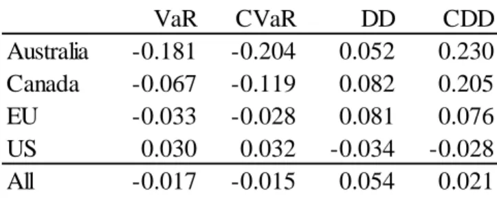
We found strong correlation (99% significance) between outcomes of the 3 different VaR and CVaR modelling techniques (parametric, historical and Monte Carlo), a key reason being our large number of historical observations, as well as the large number of forward simulations (20,000). As there is no significant difference between these methods, to avoid excessively detailed reporting we will restrict our discussion and tables to one method (parametric) for VaR and CVaR. The correlations between size and risk are shown in Table 1. None of the correlations in any of the regions are significant, and the signs differ between regions with a negative relationship for Australia, Canada and Europe, as compared to positive for the US.

Table 1. Correlation between size and risk.

The table correlates the four risk metrics, as described in sections 2 and 3, with Size (natural logarithm of total assets). It is expected that the signs for VaR/CVaR will be opposite to DD/CDD, because a higher VaR/CVar shows higher risk, whereas a higher DD/CCD shows lower risk. ** and * denote significance at the 99 and 95 percent levels respectively, whereas the absence of either of these indicators denotes no significance.

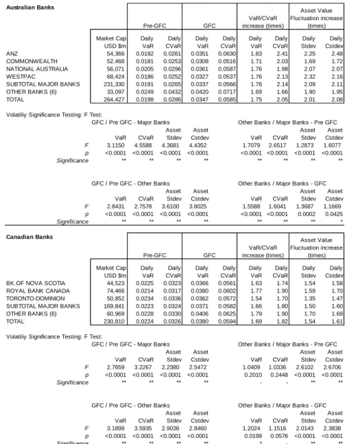
Table 2 splits the banks for all the regions into ‘major’ and ‘other’ banks and provides figures on VaR, CVaR, Stdev (asset value fluctuations) and CStdev (worst 5% of asset value fluctuations). Stdev and CStdev are the denominators for the DD and CDD (equations 7 and 9). Thus a higher Stdev(Cstdev) will correspond to a proportionately equal lower DD/CDD. Given the high number of banks (over 4 countries / regions) only ‘major’ bank figures are shown at individual level, with the ‘other’ bank figures showing the weighted average for those banks. The table also splits the figures into Pre-GFC and GFC, thus showing which category of Banks experienced greater change in risk between the two periods.

VaR CVaR DD CDD Australia -0.181 -0.204 0.052 0.230 Canada -0.067 -0.119 0.082 0.205 EU -0.033 -0.028 0.081 0.076 US 0.030 0.032 -0.034 -0.028 All -0.017 -0.015 0.054 0.021

Table 2. Risk measures for ‘major’ banks compared to ‘other’ banks.

VaR is calculated on a parametric basis, whereby the standard deviation of daily returns is multiplied by 1.645 (95% confidence level based on a normal distribution). Annual VaR can be obtained by multiplying Daily VaR by the square root of 250. Figures are undiversified and represent the weighted average of the individual bank VaRs. CVaR is calculated as the average of the worst 5% of actual returns (those beyond the 95% VaR). The GFC category calculates daily VaR for the 2 years from 2007 and 2008. The GFC category calculates daily VaR for the 7 year period from 2000-2006. ‘Major’ banks for the purposes of this table are defined as all banks with market capitalization exceeding USD $40billion. The four columns on the right of the table show the increases (GFC as compared to pre-GFC) in VaR, CVaR Asset Stdev and Asset CStdev. Market asset value of returns (Stdev) is calculated as the standard deviation of all asset returns for the period, whereas CStdev is based on the worst 5%. F testing is undertaken to test for variance in volatility. F is σ21/ σ22, where σ1 and σ2 are the standard deviations of returns for the two samples being compared. An F value of 1 shows no difference between the samples and a value of 3 shows variance of 3x higher in the one sample compared to the other. * denotes significance at the 95% level and ** at the 99% level.

Australian Banks Market Cap USD $m Daily VaR Daily CVaR Daily VaR Daily CVaR Daily VaR Daily CVaR Daily Stdev Daily Cstdev ANZ 54,366 0.0192 0.0261 0.0351 0.0630 1.83 2.41 2.25 2.48 COMMONWEALTH 52,468 0.0181 0.0253 0.0308 0.0516 1.71 2.03 1.69 1.72 NATIONAL AUSTRALIA 56,071 0.0205 0.0296 0.0361 0.0587 1.76 1.98 2.07 2.07 WESTPAC 68,424 0.0186 0.0252 0.0327 0.0537 1.76 2.13 2.32 2.16 SUBTOTAL MAJOR BANKS 231,330 0.0191 0.0265 0.0337 0.0566 1.76 2.14 2.09 2.11 OTHER BANKS (6) 33,097 0.0249 0.0432 0.0420 0.0717 1.69 1.66 1.90 1.95 TOTAL 264,427 0.0198 0.0286 0.0347 0.0585 1.75 2.05 2.01 2.08 Volatiliy Significance Testing: F Test:

GFC / Pre GFC - Major Banks Other Banks / Major Banks - Pre GFC VaR CVaR

Asset Stdev

Asset

Cstdev VaR CVaR

Asset Stdev Asset Cstdev F 3.1150 4.5588 4.3681 4.4352 1.7079 2.6517 1.2873 1.6077 p <0.0001 <0.0001 <0.0001 <0.0001 <0.0001 <0.0001 <0.0001 <0.0001 Significance ** ** ** ** ** ** ** **

GFC / Pre GFC - Other Banks Other Banks / Major Banks - GFC VaR CVaR

Asset Stdev

Asset

Cstdev VaR CVaR

Asset Stdev Asset Cstdev F 2.8431 2.7578 3.6100 3.8025 1.5588 1.6041 1.3687 1.1669 p <0.0001 <0.0001 <0.0001 <0.0001 <0.0001 <0.0001 0.0002 0.0425 Significance ** ** ** ** ** ** ** * Canadian Banks Market Cap USD $m Daily VaR Daily CVaR Daily VaR Daily CVaR Daily VaR Daily CVaR Daily Stdev Daily Cstdev BK.OF NOVA SCOTIA 44,523 0.0225 0.0323 0.0366 0.0561 1.63 1.74 1.54 1.58 ROYAL BANK CANADA 74,466 0.0214 0.0317 0.0380 0.0602 1.77 1.90 1.59 1.70 TORONTO-DOMINION 50,852 0.0234 0.0336 0.0362 0.0572 1.54 1.70 1.35 1.47 SUBTOTAL MAJOR BANKS 169,841 0.0223 0.0324 0.0371 0.0582 1.66 1.80 1.50 1.60 OTHER BANKS (6) 60,969 0.0228 0.0330 0.0406 0.0625 1.79 1.90 1.70 1.69 TOTAL 230,810 0.0224 0.0326 0.0380 0.0594 1.69 1.82 1.54 1.61 Volatiliy Significance Testing: F Test:

GFC / Pre GFC - Major Banks Other Banks / Major Banks - Pre GFC VaR CVaR

Asset Stdev

Asset

Cstdev VaR CVaR

Asset Stdev Asset Cstdev F 2.7659 3.2267 2.2380 2.5472 1.0409 1.0336 2.6102 2.6706 p <0.0001 <0.0001 <0.0001 <0.0001 0.2010 0.2448 <0.0001 <0.0001 Significance ** ** ** ** - - ** **

GFC / Pre GFC - Other Banks Other Banks / Major Banks - GFC VaR/CVaR increase (times) Asset Value Fluctuation increase (times) Pre-GFC GFC Pre-GFC GFC VaR/CVaR increase (times) Asset Value Fluctuation increase (times)

Table 2 (continued). European Banks Market Cap USD $m Daily VaR Daily CVaR Daily VaR Daily CVaR Daily VaR Daily CVaR Daily Stdev Daily Cstdev BANCO SANTANDER 121,617 0.0335 0.0482 0.0430 0.0699 1.28 1.45 1.52 1.64 BARCLAYS 48,519 0.0322 0.0473 0.0651 0.1018 2.02 2.15 3.84 4.17 BNP PARIBAS 84,755 0.0313 0.0476 0.0503 0.0812 1.61 1.70 2.68 2.92 CREDIT SUISSE 76,650 0.0393 0.0620 0.0607 0.1006 1.54 1.62 2.08 2.16 HSBC 192,500 0.0241 0.0369 0.0354 0.0588 1.47 1.60 1.68 1.90 LLOYDS TSB 50,130 0.0310 0.0455 0.0617 0.0985 1.99 2.16 3.00 2.93 SOCIETE GENERALE 45,040 0.0350 0.0511 0.0575 0.0873 1.64 1.71 2.49 2.52 UBS 72,326 0.0291 0.0435 0.0658 0.1072 2.26 2.46 3.36 3.64 UNICREDIT 50,240 0.0267 0.0411 0.0544 0.0933 2.03 2.27 3.35 3.88 SUBTOTAL MAJOR BANKS 741,777 0.0303 0.0456 0.0503 0.0818 1.66 1.79 2.05 2.22 OTHER BANKS (7) 153,969 0.0340 0.0523 0.0653 0.1118 1.92 2.14 3.61 3.92 TOTAL 895,746 0.0310 0.0468 0.0529 0.0869 1.71 1.86 2.15 2.34 Volatiliy Significance Testing: F Test:

GFC / Pre GFC - Major Banks Other Banks / Major Banks - Pre GFC VaR CVaR

Asset Stdev

Asset

Cstdev VaR CVaR

Asset Stdev Asset Cstdev F 2.7459 3.2146 4.2014 4.9261 1.2582 1.3162 8.5943 7.0611 p <0.0001 <0.0001 <0.0001 <0.0001 <0.0001 <0.0001 <0.0001 <0.0001 Significance ** ** ** ** ** ** ** **

GFC / Pre GFC - Other Banks Other Banks / Major Banks - GFC VaR CVaR

Asset Stdev

Asset

Cstdev VaR CVaR

Asset Stdev Asset Cstdev F 3.6873 4.5682 13.0506 15.3323 1.6896 1.8705 2.7668 2.2686 p <0.0001 <0.0001 <0.0001 <0.0001 <0.0001 <0.0001 <0.0001 <0.0001 Significance ** ** ** ** ** ** ** ** US Banks Market Cap USD $m Daily VaR Daily CVaR Daily VaR Daily CVaR Daily VaR Daily CVaR Daily Stdev Daily Cstdev BANK OF AMERICA 130,273 0.0268 0.0407 0.0778 0.1326 2.91 3.26 6.04 8.34 CITIGROUP 94,280 0.0306 0.0462 0.0895 0.1566 2.92 3.39 6.04 7.64 JP MORGAN 154,621 0.0361 0.0549 0.0666 0.1075 1.84 1.96 2.09 2.33 US BANCORP 43,062 0.0294 0.0460 0.0479 0.0756 1.63 1.64 1.95 2.09 WELLS FARGO 139,771 0.0213 0.0316 0.0648 0.1019 3.05 3.22 3.28 4.02 SUBTOTAL MAJOR BANKS 562,006 0.0288 0.0437 0.0711 0.1177 2.47 2.69 3.22 3.93 OTHER BANKS (46) 125,900 0.0241 0.0361 0.0638 0.1024 2.65 2.84 3.06 3.59 TOTAL 687,906 0.0279 0.0423 0.0698 0.1149 2.50 2.72 3.19 3.86 Volatiliy Significance Testing: F Test:

GFC / Pre GFC - Major Banks Other Banks / Major Banks - Pre GFC VaR CVaR

Asset Stdev

Asset

Cstdev VaR CVaR

Asset Stdev Asset Cstdev F 6.0948 7.2621 10.3795 15.4100 1.4353 1.4624 1.3362 1.1596 p <0.0001 <0.0001 <0.0001 <0.0001 <0.0001 <0.0001 <0.0001 0.0010 Significance ** ** ** ** ** ** ** **

GFC / Pre GFC - Other Banks Other Banks / Major Banks - GFC VaR CVaR

Asset Stdev

Asset

Cstdev VaR CVaR

Asset Stdev Asset Cstdev F 7.0377 8.0475 9.3722 12.8910 1.2430 1.3197 1.2066 1.0308 p <0.0001 <0.0001 <0.0001 <0.0001 0.0076 0.0010 0.0181 0.3673 Significance ** ** ** ** ** ** * -Pre-GFC GFC VaR/ CVaR increase (times) Asset Value Fluctuation increase (times) Asset Value Fluctuation increase (times) VaR/ CVaR increase (times) GFC Pre-GFC

Among the ‘majors’, Barclays, UBS, Unicredit, Bank of America, Citigroup and Wells Fargo stand out as having high VaR, CVAR and asset value fluctuations during the GFC. These are all entities which featured prominently in the GFC among those banks which suffered problems such as large losses, capital shortages, and substantial writedowns of investments in subprime mortgages. Overall, there is no clear pattern emerging as to differences in the risk measurements between ‘major’ and ‘other’ banks. In Australia, ‘major’ banks tend to have lower VaR, CVaR, Stdev, and CStdev figures than ‘other’ Banks. Both groups have significantly worse figures for all these 4 indicators during the GFC as compared to pre-GFC (significant difference at 99% confidence level using an F test), however the extent of the increase in tail risk was actually larger for the ‘majors’ (2.14x for CVaR and 2.11x for CStdev) than for ‘other’ (1.66x for CVaR and 1.95x for CStdev), which is opposite to the increases seen in Canada and Europe. The significance of the differential between CStdev for the ‘major’ banks and the ‘other’ banks in Australia falls from the 99% level pre-GFC to the 95% level during the GFC period. In Canada there is a significant differential in asset value fluctuations between ‘other’ and ‘major’ banks both pre and during the GFC, but there is no significant difference between the two groups of banks in VaR and CVaR. In Europe ‘other’ banks are more risky than ‘majors’ on all measures with this differential increasing during the GFC. In the US, the increase in all measures was fairly similar for ‘majors’ and ‘other’ banks, with GFC asset value fluctuations being similar across both groups. It should be noted of course, that as we are looking at asset value fluctuations our study only includes listed groups, and (with the notable

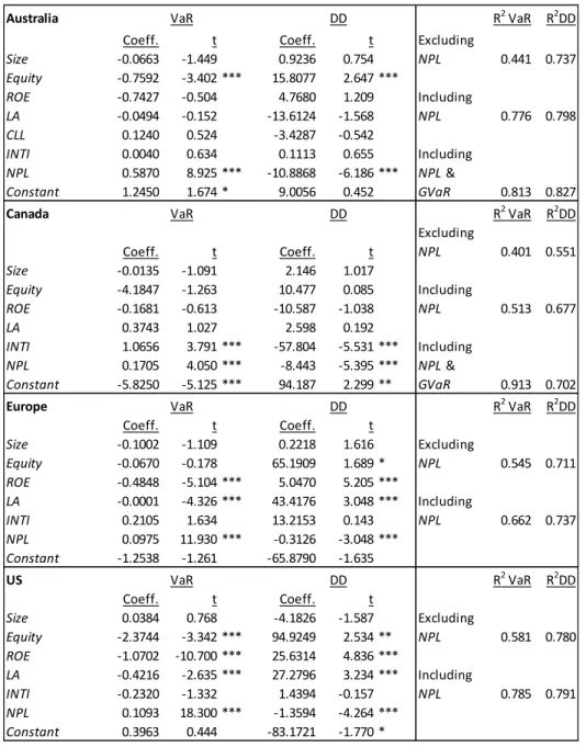
predominantly smaller unlisted entities. If we consider all 4 regions as a whole, the large increases in our risk measurements (from Pre-GFC to GFC) are widespread (but to a lesser degree in Canada and Australia), across all categories of banks in our study. Larger banks experienced significant difficulties such as access to wholesale funding (all regions), writedown of investments in sub-prime mortgages (mainly US and Europe), and exposure to corporate loan losses (all regions). Many smaller entities also had problems accessing funding. These entities generally also had relatively large exposures to the home loan market which was impacted by rising unemployment and falling house prices, particularly in the US and Europe. Many of the smaller banks also had large exposures to a falling commercial property market. Thus all categories of banks, small and large, experienced problems during the GFC. Table 3 shows the results of our fixed effects panel regression analysis as per the methodology described in Section 4.4. The discussion following the tables will show that Size is not a significant determinant of risk and that other independent variables, particularly NPL and GVaR, are much more significant than Size.

Table 3. Determinants of VaR and DD

The table shows regression results with VaR (first two numerical columns) and DD (next two numerical columns) as the dependant variables. The regression includes panel data for all the years in our dataset from with bank and time fixed effects. Dependant Variables are shown in the first column. Independent variables are defined in the paragraph preceding the table. */**/*** denote significance at the 90/95/99 percent levels respectively. R2 is shown in the final two columns of the table for VaR and DD respectively. The uppermost R2 for each region includes all independent variables except NPL. The next R2includes all the prior variables plus NPL. The final R2 includes all the independent variables, plus GVaR (which is the combined VaR figure for US and UK, and has been included to assess the impact of global events in major regions on the smaller regions of Australia and Canada).

Australia R2 VaR R2DD Coeff. t Coeff. t Size -0.0663 -1.449 0.9236 0.754 0.441 0.737 Equity -0.7592 -3.402 *** 15.8077 2.647 *** ROE -0.7427 -0.504 4.7680 1.209 LA -0.0494 -0.152 -13.6124 -1.568 0.776 0.798 CLL 0.1240 0.524 -3.4287 -0.542 INTI 0.0040 0.634 0.1113 0.655 NPL 0.5870 8.925 *** -10.8868 -6.186 *** Constant 1.2450 1.674 * 9.0056 0.452 0.813 0.827 Canada R2 VaR R2DD Coeff. t Coeff. t 0.401 0.551 Size -0.0135 -1.091 2.146 1.017 Equity -4.1847 -1.263 10.477 0.085 ROE -0.1681 -0.613 -10.587 -1.038 0.513 0.677 LA 0.3743 1.027 2.598 0.192 INTI 1.0656 3.791 *** -57.804 -5.531 *** NPL 0.1705 4.050 *** -8.443 -5.395 *** Constant -5.8250 -5.125 *** 94.187 2.299 ** 0.913 0.702 Europe R2 VaR R2DD Coeff. t Coeff. t Size -0.1002 -1.109 0.2218 1.616 Equity -0.0670 -0.178 65.1909 1.689 * 0.545 0.711 ROE -0.4848 -5.104 *** 5.0470 5.205 *** LA -0.0001 -4.326 *** 43.4176 3.048 *** INTI 0.2105 1.634 13.2153 0.143 0.662 0.737 NPL 0.0975 11.930 *** -0.3126 -3.048 *** Constant -1.2538 -1.261 -65.8790 -1.635 US R2 VaR R2DD Coeff. t Coeff. t Size 0.0384 0.768 -4.1826 -1.587 Equity -2.3744 -3.342 *** 94.9249 2.534 ** 0.581 0.780 ROE -1.0702 -10.700 *** 25.6314 4.836 *** LA -0.4216 -2.635 *** 27.2796 3.234 *** VaR DD VaR DD DD VaR Excluding NPL Including NPL Including NPL & GVaR DD VaR Including NPL Excluding NPL Excluding NPL Including Including NPL & GVaR Excluding NPL Including NPL

For all regions, the results show that size is not a significant item for any of the four

regions. Indeed, the model for all other independent variables excluding NPL and

GVaR does not provide a good explanation for VaR with R2 ranging between only 0.40 (Canada) and 0.58 (US) but a better explanation for DD ranging from 0.55

(Canada) to 0.78 (US). This increases substantially when including NPL, with VaR

ranging from 0.51 (Canada) to 0.79 (US) and DD ranging from 0.68 (Canada) to 0.79

(US). R2 increases further for Australia (VaR 0.81, DD 0.83) and Canada (VaR 0.91,

DD 0.70) when including GVaR. Although, on its own GVaR is a significant indicator

of Australian VaR and DD, when including NPL, significant R2 can be generated

from the characteristics of these banks themselves. The findings are generally consistent with the studies mentioned earlier in this section which found that (NPL aside) balance sheet and income statement factors are not a good indicator of bank

risk and that external shocks caused by global contagion (as measured by GVaR in

our study) can have a significant impact.

Across all regions, NPL is a significant determinant of VaR and PD. Equity (Australia and US) and LA (Europe and US) are significant in two regions each, but not in the

other regions. In the US and UK, ROE is more significant than in Australia and

Canada, likely because US and UK banks had significant losses over these volatile times, in line with VaR increases, whereas Australian and Canadian Banks remained profitable.

There is consistency in signs (+ or -) for all 4 regions for ROE and Equity (profitable banks with higher equity showing less risk), but no consistency among other

variables. For example, Size is positively related to risk for the US but negatively for other regions.

6. Conclusions

Neither correlation nor regression analysis show significance in association between size and risk. When splitting banks into ‘major’ banks and ‘other’ banks, size does have some significance, but the signs vary between regions. Thus, overall, the study finds no conclusive evidence of association between size and risk.

References

Acharya, V. V., Hasan, I., & Saunders, A. (2006). Should Banks be Diversified?

Evidence from Individual bank Loan Portfolios. Journal of Business, 79(3),

1355-1412.

Allen, D. E., & Powell, R. (2007). Industry Market Value at Risk in Australia.

Available at www.business.ecu.edu.au/users/dallen/wp0704da.pdf

Artzner, P., Delbaen, F., Eber, J., & Heath, D. (1999). Coherent Measures of Risk. Mathematical Finance, 9, 203-228.

Artzner, P., Delbaen, F., Eber, J. M., & Heath, D. (1997). Thinking Coherently. Risk, 10, 68-71.

Bharath, S. T., & Shumway, T. (2008). Forecasting Default with the Merton

Distance-to-Default Model. The Review of Financial Studies, 21(3),

1339-1369.

Black, F., & Scholes, M. (1973). The Pricing of Options and Corporate Liabilities. Journal of Political Economy, 81(3), 637-654.

Cornett, M. M., Ors, E., & Tehranian, H. (2002). Bank Performance Around the Introduction of a Section 20 Subsidiary Journal of Finance, 52(1), 501-521. Crosbie, P., & Bohn, J. (2003). Modelling Default Risk: Moody's KMV Company. Das, S., Duffie, D., Kapadia, N., & Saiata, L. (2007). Common Failings: How

Corporate Defaults are Correlated. The Journal of Finance, 62, 93-117. Davis, M., & Lo, V. (2001). Infectious Defaults. Quantitative Finance, 1, 382-387. De Young, R., & Roland, K. P. (2001). Product Mix and Earnings Volatility at

Commercial Banks: Evidence from a Degree of Total Leverage Model. Journal of Financial Intermediation, 10, 54-84.

Federal Deposit Insurance Corporation. (2009). Quarterly Banking Profile. Retrieved

30 August 2009. Available at http://www2.fdic.gov/qbp/index.asp

Giesecke, K., & Weber, S. (2004). Cyclical Correlations, Credit Contagion, and Portfolio Losses. Journal of Banking and Finance, 28, 3009-3096.

Giesecke, K., & Weber, S. (2006). Credit Contagion and Aggregate Losses. . Journal of Economic Dynamics and Control, 30, 741-767.

Gregoriou, G. N. (2009a). The VaR Implementation Handbook. New York: McGraw Hill.

Gregoriou, G. N. (2009b). The VaR Modeling Handbook. New York: McGraw Hill. Gropp, R., & Heider, F. (2009). The Determinants of Bank Capital Structure. Review

of Finance, 14(4), 1-36.

J.P. Morgan, & Reuters. (1994, 1996). RiskMetrics Technical Document.

Jorion, P. (1996). Value at Risk: The New Benchmark for Controlling Derivative

Jorion, P., & Zhang, G. (2007). Good and Bad Credit Contagion: Evidence from Credit Default Swaps. Journal of Financial Economics, 84, 860-883.

Kuo, H.-C., & Lee, C.-H. . (2003). The Determinants of the Capital Structure of Commercial Banks in Taiwan. 515-522. International Journal of Management, 20(4), 515 - 522.

Liao, S., & Chang, J. (2010). Economic Determinants of Default Risks and their Impacts on Credit Derivative Pricing The Journal of Futures Markets, 30(11), 1058-1081.

Lonstaff, F., & Rajan, A. (2008). An Empirical Analysis of the Pricing of Collateralized Debt Obligations. The Journal of Finance, 63, 529-563.

Ngo, P. T. H. (2008). Capital-Risk Decisions and Profitability in Banking: Regulatory

versus Economic Capital, 21st Australasian Finance and Banking

Conference.

Office of the Superintendant of Financial Institutions Canada. (2009). Financial Data - Banks. Retrieved 12 January 2010. Available at http://www.osfi-bsif.gc.ca

Pflug, G. (2000). Some Remarks on Value-at-Risk and Conditional-Value-at-Risk. In

R. Uryasev (Ed.), Probabilistic Constrained Optimisation: Methodology and

Applications. Dordrecht, Boston: Kluwer Academic Publishers.

Powell, R., & Allen, D. (2009). CVaR and Credit Risk Management. In Anderssen,

R.S., R.D. Braddock and L.T.H. Newham (eds) 18th World IMACS Congress and MODSIM09 International Congress on Modelling and Simulation. Modelling and Simulation Society of Australia and New Zealand and International Association for Mathematics and Computers in Simulation, July 2009, pp. 1508-1514.

Reserve Bank of Australia. (2009). Indicative mid rates of selected Commonwealth

Government Securities. Retrieved 19 August 2008. Available at

http://www.rba.gov.au/statistics/frequency/indicative.html

Rime, B. (2001). Capital Requirements and Bank Behaviour: Empirical Evidence from Switzerland. Journal of Banking and Finance, 25, 789-805.

Rosch, D., & Winterfeldt, B. (2008). Estimating Credit Contagion in a Standard Factor Model. Risk, 21, 78-82.

Samanta, P., Azarchs, T., & Hill, N. (2005). Chasing Their Tails: Banks Look Beyond Value-At-Risk. , RatingsDirect.

Saunders, A., & Walter, I. (1994). Universal Banking in the United States: What

Could We Gain? What Could We Lose? New York: University Oxford Press. Stiroh, K. J. (2004). Diversification in Banking: Is Noninterest Income the Answer?

Stiroh, K. J., & Rumble, A. (2006). The Darkside of Diversification: The Case of U.s. Financial Holding Companies. Journal of Banking and Finance, 30(8), 2131-2161.

Vassalou, M., & Xing, Y. (2004). Default Risk in Equity Returns. Journal of