Predictive churn models in vehicle insurance

i

Predictive Churn Models in Vehicle Insurance

Carolina Bellani

Internship report presented as partial requirement for

ob

taining the Master’s degree in

Advanced Analytics

ii

NOVA Information Management School

Instituto Superior de Estatística e Gestão de Informação

Universidade Nova de Lisboa

PREDICTIVE CHURN MODELS IN VEHICLE INSURANCE

by

Carolina Bellani

Internship report presented as partial requirement for obtaining the Master’s degree in Advanced Analytics

Advisor:Leonardo Vanneschi

Co Advisor: Jorge Mendes

iii

ABSTRACT

The goal of this project is to develop a predictive model to reduce customer churn from a company. In order to reduce churn, the model will identify customers who may be thinking of ending their patronage. The model also seeks to identify the reasons behind the customers decision to leave, to enable the company to take appropriate counter measures. The company in question is an insurance company in Portugal, Tranquilidade, and this project will focus in particular on their vehicle insurance products.

Customer churn will be calculated in relation to two insurance policies; the compulsory motor’s (third party liability) policy and the optional Kasko’s (first party liability) policy. This model will use information the company holds internally on their customers, as well as commercial, vehicle, policy details and external information (from census).

The first step of the analysis was data pre-processing with data cleaning, transformation and reduction (especially, for redundancy); in particular, concept hierarchy generation was performed for nominal data.

As the percentage of churn is not comparable with the active policy products, the dataset is unbalanced. In order to resolve this an under-sampling technique was used. To force the models to learn how to identify the churn cases, samples of the majority class were separated in such a way as to balance with the minority class. To prevent any loss of information, all the samples of the majority class were studied with the minority class.

The predictive models used are generalized linear models, random forests and artificial neural networks, parameter tuning was also conducted.

A further validation was also performed on a recent new sample, without any data leakage.

In relation to compulsory motor’s insurances, the recommended model is an artificial neural network. The model has a first layer of 15 neurons and a second layer of 4 neurons, with an AUC of 68.72%, a sensitivity of 33.14% and a precision of 27%. For the Kasko’s insurances, the suggested model is a random forest with 325 decision trees with an AUC of 72.58%, a sensitivity of 36.85% and a precision of 31.70%. AUCs are aligned with other predictive churn model results, however, precision and sensitivity measures are worse than in telecommunication churn models’, but comparable with insurance churn predictions.

Not only do the models allow for the creation of a churn classification, but they are also able to give some insight about this phenomenon, and therefore provide useful information and data which the company can use and analyze in order to reduce the customer churn rate. However, there are some hidden factors that couldn’t be accounted for with the information available, such as; competitors’ market and client interaction, if these could be integrated a better prediction could be achieved.

KEYWORDS

iv

TABLE OF CONTENTS

1. Introduction ... 1

1.1. Statement of the problem ... 1

1.2. Objective and summary of the process ... 1

1.3. Contribution to the company ... 2

2. Theoretical framework ... 3

2.1. Literature review in churn modeling ... 3

2.2. Machine Learning ... 5

2.3. Features’ pre-processing and selection ... 7

2.4. Supervised predicted models ... 9

2.4.1. Logistic regression ... 9

2.4.2. Random Forest ... 10

2.4.3. Artificial Neural Network ... 11

3. Data ... 15

4. Methodologies ... 16

4.1. Data pre-processing ... 16

4.2. Features selection ... 17

4.2.1. Set 1: Correlation-based feature selection ... 17

4.2.2. Set 2: PCA/MCA selection ... 17

4.2.3. Set 3: No features selection ... 17

4.3. Data Partition and Under-Sampling ... 18

4.4. Supervised predictive models ... 18

4.4.1. Logistic regression ... 18

4.4.2. Random Forests ... 19

4.4.3. Artificial Neural Networks... 20

4.4.4. Ensembles ... 22

4.5. Evaluation of Algorithms’ Performance ... 22

4.5.1. Re-calibration of the predicted probability ... 23

4.6. Validations ... 23

5. Results and discussion ... 24

5.1. Application of the methodology ... 24

5.2. Presentation of the results ... 27

5.2.1. Kasko’s insurance results ... 28

5.2.2. Compulsory motor insurance results ... 29

5.3. Discussion of the results ... 30

v

6. Conclusions and future works ... 32

7. Bibliography ... 34

LIST OF FIGURES

Figure 2.2 A neuron (Arora et al., 2015) ... 12

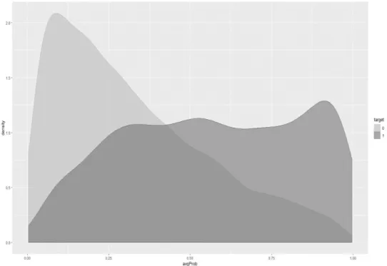
Figure 5.1 Density of the predicted probability considering the target - RF in Kasko insurances ... 27

LIST OF TABLES

Table 2.2 Evaluation Measures ... 6

Table 2.3 Correlation measures ... 8

Table 2.4 Activation functions examples ... 12

Table 4.1 Example of group aggregation... 16

Table 4.2 Parameters’ tuning in Random Forest ... 19

Table 4.3 Random Forests analysis example ... 20

Table 4.4 Example of a grid in artificial neural network’s parametrization ... 21

Table 4.5 Optimization criteria to decide the probability’s threshold ... 22

Table 5.1 Analysis of the results of GLM – compulsory insurances ... 25

Table 5.2 Train and Test measures – RF in Kasko’s insurances ... 26

Table 5.3 Lift - RF in Kasko insurances ... 27

Table 5.4 Kasko’s insurances results ... 28

vi

LIST OF EQUATIONS

Equation 2.1 Relationship between principal components and original variables ... 8

Equation 2.2 Logit function ... 9

Equation 2.3 Probability that the event occurs... 9

Equation 2.4 Odds ... 10

Equation 2.5 Logit relationship ... 10

Equation 2.6 Logistic regression ... 10

Equation 2.7 Gini measure ... 11

Equation 2.8 Cross Entropy loss function ... 13

Equation 2.9 Loss function with two regularizations ... 13

Equation 2.10 Momentum 𝜇 ... 14

Equation 4.1 Recalibration’s formula ... 23

LIST OF ABBREVIATIONS AND ACRONYMS

PCA Principal Component Analysis

MCA Multi-Correspondence Analysis

1

1.

INTRODUCTION

This report spans a six months’ internship in Tranquilidade, an insurance company. Founded in 1871, today the company is the second largest non-life insurance operator in Portugal. The task was to develop churn models for vehicle insurance policies.

1.1.

S

The generation of churn models, also known as retention or attrition models, is a growing problem in many industries. There is a frequent and increasing trend of customers switching companies in order to take advantage of a competitors’ offer. A churn model identifies the customers with a high likelihood of leaving the company. These customers cancel their contract, the policy, in order to benefit from better conditions (a lower premium) with another company. The choice in the insurance market, the fast-online simulations and the purchase methods make the customers increasingly conscious, informed and able to find cheaper opportunities.

For the company, churn prediction is one of the fundamental issues in the prevention of revenue loss and it is therefore an important way to improve competitiveness.

1.2.

O

After establishing the basics of the vehicle insurance market, the first objective was to perform data pre-processing and identify which variables will be relevant for the predictive models, taking into account potential variables’ transformations. Thereafter, validate different predictive models that identify the policies which are going to suffer consumer churn and to understand which characteristics the most affected policies have, and to understand how the models are able to solve the task.

This study focuses on vehicle policies and the churn studied is the one related to the policy’s renewal. The model’s output will give the probability of the policy to be canceled in the next annual renewal. In order to accomplish these objectives, it is possible to summarize the process in the following way:

▪ Data Pre-Processing ▪ Data Cleaning ▪ Data Transformation

▪ Data Reduction, with the selection of various variables’ sets ▪ Data Under-Sampling

▪ Predictive Models

▪ Generalized Linear Models ▪ Random Forests

▪ Artificial Neural Networks ▪ Validations

In chapter 2, there is a theoretical review. After a churn modelling literature review, the concepts of machine learning are explained. Theoretical details are outlined for each of the models employed.

2 In chapter 3, there is a general overview of the available data.

In chapter 4, the applied methodologies are shown, exploring the different steps in this study.

Results with discussions are presented in chapter 5, where there are summary tables of the best performing models. Limitations are explored at the end.

In the last chapter, 6, conclusions from the six-month internship are given.

1.3.

C

Churn prediction assists with the development and implementation of strategies for managing the company’s interactions with customers with a high risk of churn, in order to retain them. Moreover, it identifies high risk factors so they can be mitigated and brought under control.

My work during the internship, which began with the exploratory analysis, was able to give insights about the churn phenomenon and quantifies the churn risk for the considered policies.

3

2.

THEORETICAL FRAMEWORK

After a literature review in churn modeling, all the used techniques and the chosen processes are theoretically described below.

2.1.

L

The prevention of customer churn is a core Customer Relationship Management issue, known as Customer Churn Management.

In the 1990’s, (Reichheld et al., 1996) wrote that raising customer retention rates by five percentage points could increase the value of an average customer by 25 to 100 percent (in Maryland National Bank) and also determined that a 1-point increase in retention will increase the company’s capital surplus by more than 1 billion dollars over time (in State Farm - insurance). The customer loyalty’s study provides value creation, growth and consistent improvement in profit.

Also, the cost of customer retention is much lower compared to the cost of acquiring a new customer (Grönroos, 1994). It is estimated that the cost of acquiring a new customer is six times more expensive than retaining an existing one (Jobber, 2004).

As a result of the reasons above, churn management is now a major task for companies and has received increased attention.

In order to manage customer churn, it is necessary to build predictive churn models, and there are many case studies in various industries such as financial services, insurance and in the telecommunication industry in particular.

Advanced analytics, such as data mining and machine learning techniques, have been used to create churner predictions that can assist the company with customer retention.

In order to identify the most common techniques and workflows in relation to this kind of problem, a review of some related papers was completed.

KhakAbi, Gholamian, & Namvar (2010) provided a summary about data mining applications in customer churn management, showing a taxonomy based on the models employed in papers. The results show that the most commonly used technique is artificial neural network, followed in order by decision tree, logistic regression, random forest, support vector machine, survival analysis, Bayesian network, self-organizing maps and other less common techniques.

In relation to a selection of the papers, a brief review of the general context and results’ summary, citing the explored techniques, is now shown.

In Kim & Yoon (2004), by using a binomial logit model based on a survey of mobile users in Korea, the determinants of subscriber churn and customer loyalty were identified in the Korean mobile telephony market.

Burez & Van den Poel (2007), using real-life data of a European pay-tv company, employed logistic regression, Markov chains and random forests (all three with similar results) and also, proposes attrition-prevention strategies, including the study of profit quantification for the pay-tv company.

4 Mozer, Wolniewicz, Grimes, Johnson, & Kaushansky (2000) explored logit regression, decision trees, artificial neural networks and boosting techniques and based on these predictions, identified which incentives should be offered to subscribers to improve retention and maximize profitability to the carrier.

Hung, Yen, & Wang (2006) considered a Taiwan mobile operator company, and its results indicate that both decision tree and artificial neural network techniques can deliver accurate churn prediction models by using customer demographics, billing information, contract and service status, call detail records, and service change log.

Wei & Chiu (2002) investigated the churn in mobile telecommunications but from subscriber contractual information and call pattern changes extracted from call details (without customer demographics information) using decision trees, the proposed technique is capable of identifying potential churners at the contract level for a specific prediction time-period.

Zhang, Qi, Shu, & Li (2006) used decision trees, regression and artificial neural networks models and compared the models with predictors of duration of service use, payment type, amount and structure of monthly service fees and changes of the monthly service fees. It finds that duration of service use is the most predictive variable. Then payment type and other predictors about the structure of monthly service fees, especially the one within the latest 3 months, are also effective.

Coussement & Van den Poel (2008) applied support vector machines in a newspaper subscription context in order to predict the churn. Moreover, a comparison is made between two parameter-selection techniques, both based on grid search and cross-validation. Afterwards, the predictive performances of the two customized support vector machine models are compared with logistic regression and random forests performances, when the optimal hyperparameter-selection procedure is applied, support vector machines outperform traditional logistic regression, whereas random forests outperform both kinds of support vector machines.

Focusing attention on the insurance industry, it is possible to analyze the following case studies. Logistic models with some variants have been analyzed in relation to a portfolio of the largest non-life insurance company in Norway (Günther, Tvete, Aas, Sandnes, & Borgan, 2014). In particular, a logistic longitudinal regression model, which incorporates time-dynamic explanatory variables and interactions, is fitted to the data.

In Risselada, Verhoef, & Bijmolt (2010), two methods are examined; logit models and classification trees, both with and without applying a bagging procedure. Bagging consists of averaging the results of multiple models that have each been estimated on a bootstrap sample from the original sample. They test the models using the customer data of two firms from different industries, namely the internet service provider and insurance markets. The results show that the classification tree with a bagging procedure outperforms the other methods.

Based on past research, it’s apparent that a detailed theoretical framework of the machine learning concepts and algorithms is required in order to better understand the process of churn modeling.

5

2.2.

M

L

The term ‘Machine Learning’ was coined in 1959 and it is defined as a field of study in which “a computer can be programmed so that it will learn to play a better game of checkers than can be played by the person who wrote the program” (Samuel, 1959).

A more general definition can be: “a computer program is said to learn from experience ‘E’ with respect to some class of tasks ‘T’ and performance measure ‘P’, if its performance at tasks in ‘T’, as measured by ‘P’, improves with experience ‘E’” (Mitchell, 1997).

More generally, machine learning is an application of artificial intelligence and includes all the various mechanisms that provide a machine with the ability to automatically learn how to solve a specified task.

Machine learning algorithms are often categorized as supervised or unsupervised: supervised when the target variable is known and unsupervised when it is not.

One of the most common supervised tasks is classification: to be able to determine which class an object belongs to.

When there are an unequal number of objects for different classes, the dataset is said to be unbalanced. Having an unbalanced dataset makes the learning process more challenging, in the minority cases it is therefore a requirement to have a good prediction performance.

Predictive churn models are cases of supervised classification models in which the target is dichotomous and represents the churn or not churn event. In this case, the machine learning technique uses the data available to predict if the policy will be canceled and also produces a probability of customer loss occurring. In this case, the dataset has an unbalanced target; the cases’ number of churn are disproportionated with the case’s number of not-churn.

It is necessary for the machine learning models to have good generalization ability, in the case of churn classification, not only does the company want to be able to find the optimal solution in the data used to define the model, but also to generalize for as yet undefined future policies. When generalization ability is not taken into account, the model is overfitting.

In order to measure the generalization ability and the performance of the model, there are some common ways, particularly data splitting and K-cross-validation.

In data splitting, the data available is divided in two sets, training set and test set. The training set is used to create the model and the test to measure its generalization ability. Using data splitting, a problem can appear, the results are dependent on the particular set used as the training set.

To avoid this, K-cross validation is often used. The data is divided in K sets and data splitting is performed K times. Each time, one of the K sets is used as a test set and the other sets are used as training sets.

Moreover, there are some model evaluation techniques to evaluate the quality of the prediction in order to select the most suitable classification algorithm.

6 A contingency table (Table 2.1) between predicted classes and real classes is able to give a complete picture of how a classifier is performing and from it, it is possible to compute various classification metrics that can guide the models’ selection.

The target is one when an object belongs to a certain class C, zero otherwise. Table 2.1 Contingency classification table

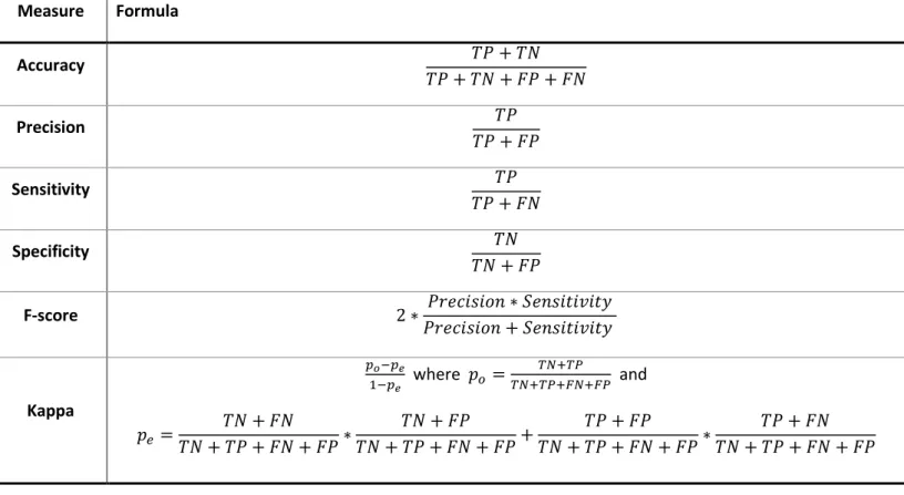
The critical measures (Table 2.2) considered for a binary classification problem are many and the most relevant are:

Table 2.2 Evaluation Measures

Measure Formula Accuracy 𝑇𝑃 + 𝑇𝑁 𝑇𝑃 + 𝑇𝑁 + 𝐹𝑃 + 𝐹𝑁 Precision 𝑇𝑃 𝑇𝑃 + 𝐹𝑃 Sensitivity 𝑇𝑃 𝑇𝑃 + 𝐹𝑁 Specificity 𝑇𝑁 𝑇𝑁 + 𝐹𝑃 F-score 2 ∗ 𝑃𝑟𝑒𝑐𝑖𝑠𝑖𝑜𝑛 ∗ 𝑆𝑒𝑛𝑠𝑖𝑡𝑖𝑣𝑖𝑡𝑦 𝑃𝑟𝑒𝑐𝑖𝑠𝑖𝑜𝑛 + 𝑆𝑒𝑛𝑠𝑖𝑡𝑖𝑣𝑖𝑡𝑦 Kappa 𝑝_𝑜−𝑝_𝑒 1−𝑝_𝑒 where 𝑝𝑜 = 𝑇𝑁+𝑇𝑃 𝑇𝑁+𝑇𝑃+𝐹𝑁+𝐹𝑃 and 𝑝𝑒= 𝑇𝑁 + 𝐹𝑁 𝑇𝑁 + 𝑇𝑃 + 𝐹𝑁 + 𝐹𝑃∗ 𝑇𝑁 + 𝐹𝑃 𝑇𝑁 + 𝑇𝑃 + 𝐹𝑁 + 𝐹𝑃+ 𝑇𝑃 + 𝐹𝑃 𝑇𝑁 + 𝑇𝑃 + 𝐹𝑁 + 𝐹𝑃∗ 𝑇𝑃 + 𝐹𝑁 𝑇𝑁 + 𝑇𝑃 + 𝐹𝑁 + 𝐹𝑃 Observed 0 1 Pr ed ic ted 0

TN

FN

FP

TP

TP (True Positives) Number of elements belonging to C and that are classified as C

TN (True Negatives) Number of elements that don't belong to C and that are not classified as C

FP (False Positives) Number of elements that don't belong to C but are classified as C

7 Another technique often used for a binary classifier system is to consider a Receiver Operating Characteristic curve (ROC curve). It is used when a classifier creates a model that outputs a numeric value, in particular a number in [0,1], and then a threshold is defined. If the output is smaller than the threshold, then the result is interpreted as class C1, otherwise as class C2. The curve is created by plotting the true positive rate (𝑇𝑃𝑅 = 𝑇𝑃

𝑇𝑃+𝐹𝑁) against the false positive rate (𝐹𝑃𝑅 = 𝐹𝑃

𝐹𝑃+𝑇𝑁) at various

values of the threshold and the considered metric is the area under this curve (AUC). Moreover, the ROC curve obtained from the model is commonly compared with the dashed line in the diagonal that represents a random predictor.

Another possible measure is the lift. Typically, numeric output of the model, with values in [0,1], is divided in deciles and for each decile, the lift is calculated. The lift is the ratio between the predicted churn rate and the real churn rate in a particular decile.

Usually the obtained churn rate is compared with the churn rate of the whole dataset to understand how much better the model is in a particular decile. It is expected that higher predicted values have better lift and that it decreases monotonously.

2.3.

F

’

-

A machine learning model uses the available data to classify the object in question. The data is a set of features and characteristics of the object that are appropriate and useful if they achieve the classification.

In the majority of cases, there are many factors influencing data quality, including accuracy, completeness, consistency, timeliness, believability and interpretability.

For this reason, it is necessary to consider data pre-processing.

The major steps (Han, Kamber, & Pei, 2012) involved in data pre-processing are: ▪ Data cleaning: missing values and resolving inconsistencies

▪ Data transformation: extraction of new or transformed features ▪ Data reduction: redundancy and relevance analysis

With data reduction, a features’ selection is usually performed. The main objectives of selection are: improving the performance, speed and cost-effectiveness of the predictors and providing a better understanding of the underlying process that generated the data. However, there are many other potential benefits such as facilitating data visualization and reducing training time.

The feature selection can be done considering the relationships between the data.

The correlation-based feature selection is a common method. It uses different correlation measures, such as Pearson, to measure the strength of the relationship with the target and the other relevant variables. The selection is done in accordance with this process, if the variables are correlated, the chosen variable will be the one with a higher correlation with the target.

In this case, the correlation measures considered are Pearson, Spearman, Cramér’s V and Information Value (Table 2.3).

8 Table 2.3 Correlation measures

Correlation Formula

Pearson _𝜌

𝑥,𝑦=

𝑐𝑜𝑣(𝑥,𝑦) √𝑣𝑎𝑟(𝑥)√𝑣𝑎𝑟(𝑦),

where 𝑐𝑜𝑣 is the covariance and 𝑣𝑎𝑟 is the variance.

Spearman _𝑟

𝑠= 𝜌𝑟𝑔_𝑥,𝑟𝑔_𝑦=

𝑐𝑜𝑣(𝑟𝑔𝑥,𝑟𝑔𝑦) √𝑣𝑎𝑟(𝑟𝑔𝑥)√𝑣𝑎𝑟(𝑟𝑔𝑦),

where 𝑐𝑜𝑣 is the covariance, 𝑣𝑎𝑟 is the variance and 𝑟𝑔𝑥 is the rank

variable 𝑥. Cramér’s V 𝑉 = √ 𝜒2 2 ⁄ min (𝑘−1,𝑟−1),

where 𝜒2 is the chi-squared statistics, 𝑘 the number of columns and 𝑟 the number of rows.

Information Value 𝐼𝑉 = ∑𝑘𝑖=1(% 𝑜𝑓 𝑛𝑜 𝑒𝑣𝑒𝑛𝑡 − % 𝑜𝑓 𝑒𝑣𝑒𝑛𝑡) ∗ 𝑊𝑂𝐸𝑖,

where the weight of evidence 𝑊𝑂𝐸𝑖 = ln (

% 𝑜𝑓 𝑛𝑜𝑛−𝑒𝑣𝑒𝑛𝑡

% 𝑜𝑓 𝑒𝑣𝑒𝑛𝑡𝑠 ) and 𝑘 is the

number of bins/categories of which the variable is characterized.

Another common method is the Principal Component Analysis/Multi-Correspondence Analysis (PCA/MCA) feature selection; PCA when the variables are quantitative and MCA when they are qualitative.

The goal of PCA is to summarize the information contained in the quantitative data, with a new set of variables called principal components. These new variables are uncorrelated and are ordered so that the first of them accounts for most of the variation in all the original variables.

The problem is to find a linear combination of the original variables such that the first component maximizes the explained variance. Afterwards, the problem is to find the second component that maximizes the remaining variance and is orthogonal to the first one and so on until the 𝑛𝑡ℎcomponent. Prior to this, it is a suggested practice to standardize the variables to be able to compare the contribution to the component of each variable.

Considering Y as the new components and X as the original variables, the problem is to find a linear combination:

𝑌1 = 𝑒11𝑋1 + 𝑒12𝑋2+··· +𝑒1𝑝𝑋𝑝

𝑌2 = 𝑒21𝑋1 + 𝑒22𝑋2+··· +𝑒2𝑝𝑋𝑝

…

𝑌𝑝 = 𝑒𝑝1𝑋1 + 𝑒𝑝2𝑋2+··· +𝑒𝑝𝑝𝑋𝑝

9 such that:

• 𝑉𝑎𝑟(𝑌𝑚) = ∑𝑘=1𝑝 ∑𝑝𝑖=1𝑒𝑚𝑖𝑒𝑚𝑘𝜎𝑖𝑘 = 𝑒𝑚𝑇𝛴𝑒𝑚 is maximized considering the remaining

variance for each component m;

• 𝑒𝑚𝑇𝑒𝑚= 1

• The components are uncorrelated.

It is possible to observe that𝑉𝑎𝑟(𝑌𝑗) = 𝑉𝑎𝑟(𝑒𝑗1𝑋1+𝑒𝑗2𝑋2+…+𝑒𝑗𝑝𝑋𝑝) = 𝜆𝑗.

Moreover, if it is necessary to reduce the dimensionality, different cut-offs could be used: it is common to have as many components as there are eigenvalues greater than one. Also, it is possible to consider as many components as possible to explain a certain cumulative variance.

Instead, Multi-Correspondence Analysis (MCA) (Yelland, 2010) is an extension of the PCA for analyzing contingency tables of categorical variables. At the start, a chi-square test is performed and given the significance of it, it is possible to show these relations graphically.

In this case, the analysis can understand the behavior of different groups of the categorical variables (column analysis) and the behavior of the policies (row analysis).

The goal of MCA is to create a new set of variables, using the categorical ones, that will be orthogonal and continuous.

2.4.

S

As logistic regressions, random forests and artificial neural networks are often cited in churn prediction papers and because they are common binary classification algorithms, these models were explored, and in this section it is possible to find their theoretical review.

2.4.1.

Logistic regression

Generalized Linear Models are a class of statistical model that are a generalization of the classical linear ones: they use a link function to model a relationship between a response binary variable and a set of independent variables. There are many link functions and, in this case, the logit function is used. The logit function is defined as:

𝑙𝑜𝑔𝑖𝑡(𝑥) = log ( 𝑥 1 − 𝑥) Equation 2.2 Logit function

A binary logistic model has a dependent variable with two possible values: in this case, 1 if the policy is canceled, and 0 if it is not cancelled.

It is possible to define the probability of the presence of the event for each considered object 𝑖: 𝑝𝑖 = 𝑃(𝑌𝑖 = 1)

10 Also, it is possible to define the odds of the event taking place.

𝑂𝑑𝑑𝑠 = 𝑃(𝑌𝑖 = 1)

1 − 𝑃(𝑌𝑖 = 1)

= 𝑝𝑖

1 − 𝑝𝑖

Equation 2.4 Odds

The logistic regression generates the coefficients of a formula to predict the logit transformation of the probability of the considered event’s presence (churn event) considering the predictors’ linear combination:

𝑙𝑜𝑔𝑖𝑡(𝑝𝑖) = log (

𝑝𝑖

1 − 𝑝𝑖

) = 𝛽0+ 𝛽1𝑋1+ ⋯ + 𝛽𝑛𝑋𝑛

Equation 2.5 Logit relationship

Then, using logistic regression it is possible to calculate the probability for each object 𝑖 that the event occurs:

𝑝𝑖 = 𝑃(𝑌𝑖 = 1) = 𝜆(𝛽0+ 𝛽1𝑋1+ ⋯ + 𝛽𝑛𝑋𝑛)

with𝜆 logistic function: 𝜆(𝑥) = 1

1+𝑒−(𝑥)

Equation 2.6 Logistic regression

In churn model and considering the policy’s churn, 𝑝𝑖 is the churn probability for each policy and the

predictors 𝑋1, 𝑋2… 𝑋𝑛 are the selected features.

Logistic regression is very appealing for different reasons: it is well known and frequently used, it has easy interpretation of the logit and generally provides good and robust results that may even outperform more sophisticated methods.

2.4.2.

Random Forest

Decision trees have become very popular for solving classification tasks, easy to use and to interpret. As logistic regressions, a decision tree’s goal is to create a model that predicts the value of a target variable based on several input variables.

Decision trees can also be represented as sets of if-then rules; the instance classification is done through the tree, from the root to the leaf node. Leaves represent the class labels and branches represent conjunctions of features that lead to those class labels.

However, they usually have a lack of robustness and suboptimal performance, they tend towards overfitting.

Random forests are an ensemble, a combination of tree predictors, each tree gives a classification and the forest chooses, taking into consideration all the votes. This gives the random forests the ability to correct the decision trees’ habit of overfitting.

11 Each tree of the random forest is grown as follows (Breiman, 2001):

▪ If the number of cases in the training set is N, sample N cases at random, but with replacement from the original data. This sample will be the training set for growing the tree.

▪ If there are M input variables, a number m<<M is specified such that at each node, m variables are selected at random out of the M and the best split, on the m variables, is used to split the node. The value of m is held constant during the forest growth.

▪ Theoretically, each tree could grow to the largest possible extent (in this application, a minimum node size is considered).

To choose the best split, a measure to quantify the usefulness of a variable is necessary.

In this case, the Gini criterion is chosen; the variable, which causes the maximum decrease in the Gini, is the chosen variable for that split.

The computation of the Gini measure for a set of objects with 𝐽 classes is: 𝐺𝑖𝑛𝑖 = 1 − ∑ 𝑝𝑖2

𝐽

𝑖=1

Equation 2.7 Gini measure

where 𝑝𝑖is the proportion of objects in which the target class is equal to 𝑖. The minimum Gini’s value

is equal to zero: when the objects belong to just one class the second term of Equation 2.7 is one and the final Gini is zero, the node represents just that class and then there is a perfect separation of the class in the node, using the split. In the binary target case, the maximum Gini is 0.5, this occurs when the classes are half of one class and half of another.

2.4.3.

Artificial Neural Network

Artificial neural networks are computational techniques biologically inspired, they try to reproduce a simplified model of the human brain. As the brain is composed of neurons, these systems are also based on a collection of connected artificial neurons. In these models, a single neuron is only able to perform small tasks, but the synergy of many neurons is able to solve complex problems.

There are different types of artificial neural networks depending on their architecture. The architecture defines how the neurons interact and how they are linked.

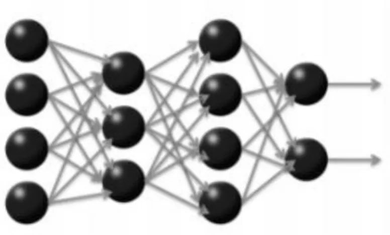
In this application, multi-layer feed-forward artificial neural networks (Figure 2.1) are explored. Their main characteristics are that the neurons in a given layer receive as input the outputs of the neurons of the previous level, there are no inter-level connections and all the possible intra-level connections exist between two subsequent layers.

12 Figure 2.1 A multi-layer feed-forward artificial neural network (Arora et al., 2015)

To understand better, it is possible to consider an artificial neural network with a single neuron, before expanding that understanding to consider further neurons.

In Figure 2.2, it is possible to notice that the neuron receives the inputs, the selected features and a bias (a 1-constant feature), through the weights. The output 𝑓(∑𝑛𝑖=1𝑤𝑖∗ 𝑥𝑖+ 𝑏) is a function of the

inputs called an activation function. In table 2.4, there are some activation function examples. Table 2.4 Activation functions examples

Function Formula Range

Tanh 𝑓(𝛼) =𝑒

𝛼_{− 𝑒}−𝛼

𝑒𝛼_{+ 𝑒}−𝛼 𝑓(∙) 𝜖 [−1, 1]

Logistic 𝑓(𝛼) = 1

1 + 𝑒−𝛼 𝑓(∙) 𝜖 (0, ,1)

Rectified Linear 𝑓(𝛼) = max (0, 𝛼) 𝑓(∙) 𝜖 ℝ+

Maxout 𝑓(𝛼1, 𝛼2) = max (𝛼1, 𝛼2) 𝑓(∙) 𝜖 ℝ

13 The weights are parameters that need to be identified in order to achieve the task, and a learning rule is the algorithm that modifies these parameters. In particular, learning occurs when the connections and weights are adapted to minimize the error on the labeled training data. Then, the goal is to minimize the loss function for each object 𝑗 in consideration, 𝐿(𝑊, 𝐵 | 𝑗) where 𝑊 represents the weight matrix and 𝐵 the biases.

For classification tasks, a possible appropriate loss function is the Cross Entropy: 𝐿(𝑊, 𝐵 | 𝑗) = − ∑(ln (𝑜𝑦(𝑗)) ∗ 𝑡𝑦(𝑗)+ ln (1 − 𝑜𝑦(𝑗)) ∗ (1 − 𝑡𝑦(𝑗)))

𝑦∈𝑂

Equation 2.8 Cross Entropy loss function

where 𝑡(𝑗)and 𝑜(𝑗)are respectively the target and the predicted output for the j object, 𝑦 the output unit and 𝑂 the output layer.

Commonly, in order to prevent overfitting, two regularizations techniques are introduced in the error formula: 𝜆1 (Lasso) and 𝜆2 (Ridge). They modify the loss function such that:

𝐿0(𝑊, 𝐵 | 𝑗) = 𝐿(𝑊, 𝐵 | 𝑗) + 𝜆1∗ 𝑅1(𝑊, 𝐵 | 𝑗) + 𝜆2∗ 𝑅2(𝑊, 𝐵 | 𝑗)

Equation 2.9 Loss function with two regularizations

Where 𝑅1(𝑊, 𝐵 | 𝑗) represents the sum of all the norms of the weights and biases and 𝑅1(𝑊, 𝐵 | 𝑗)

represents the sum of the square of all the weights norms.

In this case, the learning algorithm considered is a parallelized version of stochastic gradient descent (SGD).

A summary of standard SGD is (LeCun, Bottou, Orr, & Müller, 1998): ▪ Initialize 𝑊, 𝐵

▪ Iterate until convergence criterion reached: 2.1. Get training example 𝑖

2.2. Update all weights 𝑤𝑗𝑘𝜖 𝑊, biases 𝑏𝑗𝑘𝜖 𝐵

𝑤𝑗𝑘 ≔ 𝑤𝑗𝑘− 𝛼 𝛿𝐿(𝑊, 𝐵 | 𝑗) 𝛿𝑤𝑗𝑘 𝑏𝑗𝑘 ≔ 𝑏𝑗𝑘− 𝛼 𝛿𝐿(𝑊, 𝐵 | 𝑗) 𝛿𝑏𝑗𝑘

With 𝛼, learning rate and 𝐿(𝑊, 𝐵 | 𝑗) computed via backpropagation.

In this application, A parallelization scheme (called HOGWILD!) is used (Niu, Recht, Re, & Wright, 2011): 1. Initialize global model parameters 𝑊, 𝐵

2. Distribute training data 𝑇 across nodes (can be disjointed or replicated) 3. Iterate until convergence criterion reached:

14 a) Obtain copy of the global model parameters 𝑊𝑛, 𝐵𝑛

b) Select active subset 𝑇𝑛𝑎 ⊂𝑇𝑛 (user-given number of samples per iteration)

c) Partition 𝑇𝑛𝑎 into 𝑇𝑛𝑎𝑐 by cores 𝑛𝑐

d) For cores 𝑛𝑐 on node n, do in parallel:

(I) Get training example 𝑖 𝜖 𝑇𝑛𝑎𝑐

(II) Update all weights 𝑤𝑗𝑘𝜖 𝑊𝑛, biases 𝑏𝑗𝑘 ∈ 𝐵𝑛

𝑤𝑗𝑘 ≔ 𝑤𝑗𝑘− 𝛼 𝛿𝐿(𝑊, 𝐵 | 𝑗) 𝛿𝑤𝑗𝑘 𝑏𝑗𝑘 ≔ 𝑏𝑗𝑘− 𝛼 𝛿𝐿(𝑊, 𝐵 | 𝑗) 𝛿𝑏𝑗𝑘 3.2. Set 𝑊, 𝐵 := 𝐴𝑣𝑔𝑛 𝑊𝑛, 𝐴𝑣𝑔𝑛 𝐵𝑛

Moreover, in the learning algorithm, it is possible to add other advanced optimization parameters such as momentum and learning rate annealing.

Momentum modifies the weights’ modification by allowing prior iterations to influence the current version in order to prevent getting stuck in local minima:

𝑣𝑡+1 ≔ 𝜇𝑣𝑡− 𝛼𝛻𝐿(𝑤𝑡)

𝑤𝑡+1 ≔ 𝑤𝑡+ 𝑣𝑡+1

Equation 2.10 Momentum 𝜇

During the training, it is also convenient to modify the learning rate, gradually reducing it, to be able to control the minima’s approach.

In this application, ADADELTA method (D. Zeiler, 2012) is used. This method dynamically adapts the weights’ modification over time, combining the benefits of learning rate annealing and momentum.

15

3.

DATA

The analysis was performed on the policies with no payment in the renewal, any other reasons were excluded, for example, cancelation for excess of claims. The considered renewal timeline was from January to October 2017. Finally, a further validation of the models’ performances was completed from January to December 2018.

Only personal insurances were considered and for light vehicles, passenger and duty trucks. The available information could be divided in six different macro groups:

▪ Client’s and conductor’s information: sex, age, driver license’s date, location, loyalty program and customer’s tenure;

▪ Vehicle information: brand, model, engine size, cubic capacity, number of seats, combustible type, car’s year and identification number;

▪ Policy information: tenure, month of renewal, type of option, frequency of the payment, payment method, type of policy with different indicator variants and processed information from the company. Processed information from the company is the premium of the year before and the year after, the bonus/malus percentage amount due to claims, the discount percentage from the standard price and the price zone established due to an internal system. With indicator variants, it is possible to know if the client buys supplementary coverages. ▪ Commercial information: where the policy was bought, with which channel, the percentage of

positive simulations made by the client with his/her channel, and the portfolio of that channel. ▪ Other policies’ information: which kind of company policies the customer has, for example if

he/she has health insurance. ▪ Census information.

All the internal information available could be considered as 92 variables and the census information had an additional 123 variables. The 2017 portfolio of 10 months had 197,110 policies.

16

4.

METHODOLOGIES

4.1.

D

-

This chapter will explore data cleaning, transformation and reduction as they were utilised in this process, and below it is possible to find the detailed descriptions of their application.

In data cleaning, in order to use the company information, the client and conductor data were combined to create new more consistent and complete features. In many cases (more than 90%) the policy holder is also the driver. During the client’s registration in the company database, more attention is given to the driver information; for this reason, if there is incoherence between the driver and client data, the first one is eligible as the most accurate. It was possible to check the consistency between age, driver license’s age and client’s tenure.

Features with more than 15% of missing values were not considered. Other missing values were imputed using different methods. Metric missing values were filled by the median and by median considering groups, for example, the missing populational density was imputed considering the median by districts. Non-metric missing values were filled, instead, considering the mode by groups with the target behavior or decision tree imputations. In this last method, a decision tree, with the cancelation indicator as a target, shows a ramification in which the missing values is grouped with an existent level of the non-metric variables.

In data transformation for nominal data, a definition of concept hierarchies was explored, which leads to granularity loss but enables a better general comprehension.

To achieve this, it is possible to use conditional inference trees. The algorithm works as follows (Hothorn, Hornik, & Zeileis, 2006):

▪ Test the global null hypothesis of independence between the input variable and the response. Stop if this hypothesis cannot be rejected. This association is measured by a p-value.

▪ Implement a binary split in the variable.

▪ Recursively repeat until a termination condition is violated

This step was fundamental because many no-metric variables have a lot of categories. In addition, all the aggregated features were analyzed; the different new groups have differences in the churn rate and in the same group we have categories with the same behavior (Table 4.1).

Table 4.1 Example of group aggregation

Variable Variables' Categories

Aggregated

Groups Churn Rate

Policies' Percentage Variable Level1 Group1 10.11% 28.06% Level2 Group1 10.83% 8.03% Level3 Group1 11.12% 7.27% Level4 Group2 12.55% 4.96% Level5 Group2 12.56% 22.19% Level6 Group2 12.59% 24.06%

17 Other groups were created following the meaning of the variable itself: for example, the different districts were aggregated following the geographical position.

Also, the numerical variables are transformed into categorical variables; it is expected that in a value range the churn rate has the same behavior.

Considering the external information from census, some variables were binned with a decision tree; although, the decision tree didn’t show any ramifications for some of them and these variables will not help to predict the target, but further considerations will be done in the following steps.

In order to achieve data reduction:

▪ Considering the quantitative variables, it is possible to measure the relationship with Pearson and Spearman coefficients.

▪ Considering the qualitative variables, it is possible to perform a Chi-Square test to know if two variables are dependents and to measure the relationship with Cramér’s V coefficient. Also, Information Value measure will be considered in order to measure the importance of variables related to the prediction of the target.

4.2.

F

Redundancy and relevance can influence the performance of the models, therefore different feature selections are explored.

▪ Set 1: Correlation-based

▪ Set 2: Principal Correspondent Analysis and Multi-Correspondence Analysis ▪ Set 3: No feature selection

4.2.1.

Set 1: Correlation-based feature selection

Considering the correlation, it is possible to identify a set of variables that could explain the target well, but they are not correlated between them. If the variables are correlated, the chosen variable will have a higher correlation with the target; considering Pearson and/or Spearman correlation for the quantitative variables and Cramér’s V and/or Information Value for the qualitative variables. If the variable, after data transformation, has double nature (numerical and categorical), the selection must take into consideration the performance of the models.

4.2.2.

Set 2: PCA/MCA selection

In Principal Component Analysis, the inputs are quantitative variables and in Multi-Correspondence Analysis, the inputs are qualitative variables. The output is a new set of orthogonal variables: the number of variables selected are chosen considering the percentage of explained variance.

4.2.3.

Set 3: No features selection

Models, that allow a lot of correlated variables such as Random Forest, have been run trying to consider as few transformations as possible, and as few selections as possible.

18 It is expected that the results will be the worst, but this will show if some selections or some transformations are weakening the predictors, or if some important information is not being considered.

4.3.

D

P

U

-S

As discussed in the machine learning’s theoretical framework, the data splitting method is required to evaluate the models’ performance.

Accounting for the target distribution(stratified the sets), the data is divided in: ▪ Training Set (70%): the models will be derived based on this set

▪ Test Set (30%): the models will be tested in this set and the results will be compared with the real target, taking into consideration various measures such as specificity and precision. Considering the training, because the percentage of canceled policies is not equal to the active ones, the dataset is unbalanced: having unbalanced classes makes the prediction of the rare cases, the churn ones, a more complex problem. Under-sampling techniques are used to face this problem.

With this technique, the active policies will be divided to create groups comparable in size to the canceled policies (50% active policies, 50% canceled policies) and the prediction’s process will be:

▪ Training every time with the same canceled policies vs the group of active policies

▪ The final classification will be done considering an ensemble of the different trained models To summarize, in the training set there are 7 different samples where the target is balanced (almost 50-50) when using the under-sampling technique. The fixed process for each algorithm is to fit different models in the 7 samples and to consider the final model an ensemble of these 7 models for each algorithm.

4.4.

S

As the theoretical framework shows, the considered models are logit models, random forests and artificial neural networks. To understand and to improve the models, different analysis and parametrizations were completed. In the following sections the methodologies used in each model are explained.

4.4.1.

Logistic regression

After noticing that the numerical variables were not following a linear relationship with the odds ratio of the predicted probabilities, and therefore required complex transformations, a model with only categorical variables was selected.

Considering a balanced sample in the train and the variables of correlation-based selection, a further reduction was applied, both considering the overall variable’s significance from a Chi-Square test and the levels’ significance from a Z-test.

The analysis was done for the seven models and the evaluation was done both singularly for the seven models and both for the ensembles.

19

4.4.2.

Random Forests

All the variables from correlation-based selection are considered, but with some repetitions. The same variable could be considered several times as numerical and with its various transformations. To select the suitable transformation (or no transformation), a naïve random forest is used: the transformation with the most decrease of the Gini’s mean is considered. The mean decrease Gini is based on the decrease of Gini impurity. For each variable, the sum of the Gini decreases across every tree of the forest and it is accumulated every time that the variable is chosen to split a node; the sum is divided by the number of trees in the forest to give an average. Its scale is irrelevant and only the relative values matter.

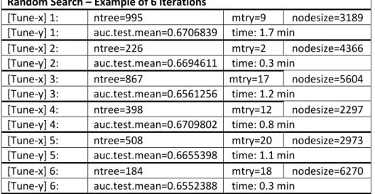
After the variables’ decision, a random search to select the parameters was performed. A grid of the potential parameters was decided: number of trees, number of variables at each split, and node’s size. One of the seven balanced training samples was further partitioned in training and validation set. The random search, with 3-fold cross validation and with 100 random parameter combinations, was performed and the parametrization with the highest AUC was selected. It is possible to see an example of parameters, and their space with 6 iterations of a random search, in Table 4.2.

The seven models were fitted with the chosen parametrization and their performance, as well as their ensemble, are evaluated.

Table 4.2 Parameters’ tuning in Random Forest

Parameters Space

ntree 50 to 1e+03

mtry 2 to 20

nodesize 2e+03 to 9e+03

Random Search – Example of 6 iterations

[Tune-x] 1: ntree=995 mtry=9 nodesize=3189

[Tune-y] 1: auc.test.mean=0.6706839 time: 1.7 min

[Tune-x] 2: ntree=226 mtry=2 nodesize=4366

[Tune-y] 2: auc.test.mean=0.6694611 time: 0.3 min

[Tune-x] 3: ntree=867 mtry=17 nodesize=5604

[Tune-y] 3: auc.test.mean=0.6561256 time: 1.2 min

[Tune-x] 4: ntree=398 mtry=12 nodesize=2297

[Tune-y] 4: auc.test.mean=0.6709802 time: 0.8 min

[Tune-x] 5: ntree=508 mtry=20 nodesize=2973

[Tune-y] 5: auc.test.mean=0.6655398 time: 1.1 min

[Tune-x] 6: ntree=184 mtry=18 nodesize=6270

[Tune-y] 6: auc.test.mean=0.6552388 time: 0.3 min

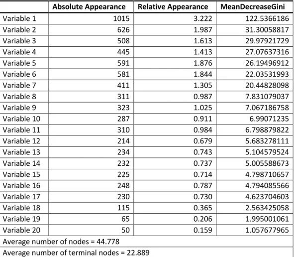
Together with the evaluation metrics, these models were also studied with consideration to the absolute and relative appearance of the variables (that doesn’t give any information about its importance, because it can happen that the variable appears just a few times, but in critical splits) and the importance considering the decrease of Gini measure. Also, the structure of the decision trees

20 (how many nodes and how many terminal nodes) was considered. In table 4.3 there is an example of this analysis.

Table 4.3 Random Forests analysis example

Absolute Appearance Relative Appearance MeanDecreaseGini

Variable 1 1015 3.222 122.5366186 Variable 2 626 1.987 31.30058817 Variable 3 508 1.613 29.97921729 Variable 4 445 1.413 27.07637316 Variable 5 591 1.876 26.19496912 Variable 6 581 1.844 22.03531993 Variable 7 411 1.305 20.44828098 Variable 8 311 0.987 7.831079037 Variable 9 323 1.025 7.067186758 Variable 10 287 0.911 6.99071235 Variable 11 310 0.984 6.798879822 Variable 12 214 0.679 5.683278111 Variable 13 234 0.743 5.104579524 Variable 14 232 0.737 5.005588673 Variable 15 225 0.714 4.798710657 Variable 16 248 0.787 4.794085566 Variable 17 230 0.730 4.623704603 Variable 18 115 0.365 2.563425058 Variable 19 65 0.206 1.995001061 Variable 20 50 0.159 1.057677965

Average number of nodes = 44.778

Average number of terminal nodes = 22.889

4.4.3.

Artificial Neural Networks

After some other data preparation such as scaling and encoding, the variable based-correlation selection was considered.

The input nodes correspond to the processed features and some fixed decisions were taken: ▪ The linkages are feed-forward and they are dense

▪ The error function, since it is a classification problem, is the cross entropy ▪ The output activation function, since the target is binary, is the sigmoid function

The other parameters were tuning, considering a random search with 3-fold cross validation and the maximization of the AUC.

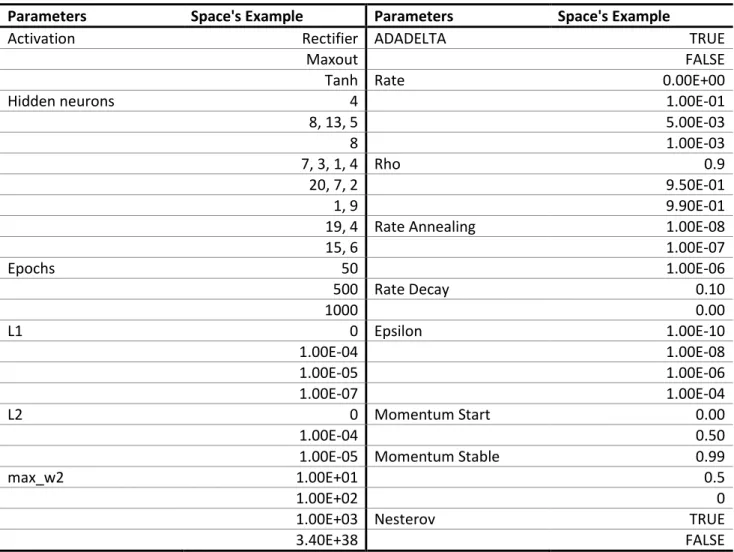
As the space of the possible combinations is large, different random searches with 100 iterations were tested. In particular, the grid was composed by:

21 ▪ For each search, a list of possible neurons was generated; each element of the list had a variable length, such that both the number of neurons and the number of layers was parametrized

▪ L1 and L2 error regularizations with the weights’ norm ▪ Activation functions

▪ Learning algorithm; in this case, the used package (Arora et al., 2015) was offering two different possibilities.

▪ Using ADADELTA algorithm

▪ Using a personalized algorithm with the parametrization of rate (learning rate), rate decay (rate decay factor between layers), rho (adaptive learning rate time decay factor), epsilon (adaptive learning rate time smoothing factor to avoid dividing by zero), stable momentum, start momentum and the use of Nesterov, accelerated gradient method.

Table 4.4 Example of a grid in artificial neural network’s parametrization

Parameters Space's Example Parameters Space's Example

Activation Rectifier ADADELTA TRUE

Maxout FALSE

Tanh Rate 0.00E+00

Hidden neurons 4 1.00E-01

8, 13, 5 5.00E-03

8 1.00E-03

7, 3, 1, 4 Rho 0.9

20, 7, 2 9.50E-01

1, 9 9.90E-01

19, 4 Rate Annealing 1.00E-08

15, 6 1.00E-07 Epochs 50 1.00E-06 500 Rate Decay 0.10 1000 0.00 L1 0 Epsilon 1.00E-10 1.00E-04 1.00E-08 1.00E-05 1.00E-06 1.00E-07 1.00E-04 L2 0 Momentum Start 0.00 1.00E-04 0.50

1.00E-05 Momentum Stable 0.99

max_w2 1.00E+01 0.5

1.00E+02 0

1.00E+03 Nesterov TRUE

3.40E+38 FALSE

22 For the two universes, two artificial neural networks with ADADELTA and one artificial neural network with personalized learning algorithms were studied.

4.4.4.

Ensembles

Different ensembles of the models were tested, including average, median and majority vote (considering two different cut-offs to decide the majority cases).

4.5.

E

A

’

P

The evaluation of the models was completed by applying them to the complete train and the test sets. The contingency table of the predicted churn and real churn was considered, together with the following measures: accuracy, precision, sensitivity, specificity, kappa, F-score, AUC and Lift.

Particular importance is given to precision and sensitivity; they are inversely proportioned but both crucial.

The evaluation measures are calculated for the different possible thresholds of the predicted probabilities.

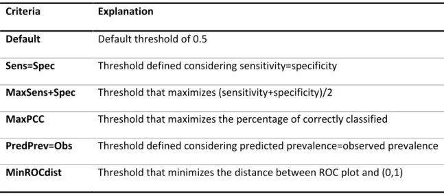
Different optimal threshold choices relating to different optimization criteria were considered, the final one used is the one using the maximization of Kappa measure. The other criteria are shown in Table 4.5.

Table 4.5 Optimization criteria to decide the probability’s threshold

Criteria Explanation

Default Default threshold of 0.5

Sens=Spec Threshold defined considering sensitivity=specificity

MaxSens+Spec Threshold that maximizes (sensitivity+specificity)/2

MaxPCC Threshold that maximizes the percentage of correctly classified

PredPrev=Obs Threshold defined considering predicted prevalence=observed prevalence

MinROCdist Threshold that minimizes the distance between ROC plot and (0,1)

In addition, it was graphically studied the distribution of the predicted probabilities by the real target; ideally the distribution of the real cancelations have high probabilities and the distribution of no cancelations have low ones.

Also, the absolute average error between the predicted probabilities and the churn rate considering the levels of the variables, used in the models and not, were studied to understand where the models is able to predict well in average and in which categories.

23

4.5.1.

Re-calibration of the predicted probability

As a result of the under-sampling techniques, a recalibration of the predicted probability is required. Adjusting the probability to account for the different proportions in the training and in the test set could cause an error. The sum of the probability to be one and to be zero do not sum up to one. For this reason, the calibration needs to be done in the space of the odds ratio in the following way:

𝑂𝑟𝑖𝑔𝑖𝑛𝑎𝑙_𝑜𝑑𝑑𝑠 = 𝐶ℎ𝑢𝑟𝑛_𝑃𝑟𝑜𝑏𝑎𝑏𝑖𝑙𝑖𝑡𝑦_𝑈𝑛𝑏𝑎𝑙𝑎𝑛𝑐𝑒𝑑 1 − 𝐶ℎ𝑢𝑟𝑛_𝑃𝑟𝑜𝑏𝑎𝑏𝑖𝑙𝑖𝑡𝑦_𝑈𝑛𝑏𝑎𝑙𝑎𝑛𝑐𝑒𝑑 𝑈𝑛𝑑𝑒𝑟𝑠𝑎𝑚𝑝𝑙𝑖𝑛𝑔_𝑜𝑑𝑑𝑠 = 𝐶ℎ𝑢𝑟𝑛_𝑃𝑟𝑜𝑏𝑎𝑏𝑖𝑙𝑖𝑡𝑦_𝐵𝑎𝑙𝑎𝑛𝑐𝑒𝑑 1 − 𝐶ℎ𝑢𝑟𝑛_𝑃𝑟𝑜𝑏𝑎𝑏𝑖𝑙𝑖𝑡𝑦_𝐵𝑎𝑙𝑎𝑛𝑐𝑒𝑑 Scoring_odds_𝑖 = Predicted_Probability𝑖 1 −Predicted_Probability_𝑖 Adjusted_odds_𝑖 =Scoring_odds𝑖∗ 𝑂𝑟𝑖𝑔𝑖𝑛𝑎𝑙_𝑜𝑑𝑑𝑠 𝑈𝑛𝑑𝑒𝑟𝑠𝑎𝑚𝑝𝑙𝑖𝑛𝑔_𝑜𝑑𝑑𝑠 Adjusted_Probability_𝑖 = 1 1 + 1⁄Adjusted_odds_𝑖

Equation 4.1 Recalibration’s formula

4.6.

V

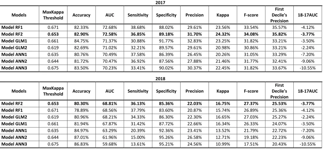
In the case of a new sample becoming available, it is possible to validate the model using this new data. Moreover, with a new sample, the presence of data leakage can be tested, when information from outside of the training dataset is used to create the model.

The new sample is from 2018. In this year, the number of policies more than doubled and the churn rate has a slight difference.

In the validation analysis, the comparison was performed using the models with the highest AUC in 2017. All the experimented models are an ensemble of the 7 under-samples, and some are also an ensemble of different algorithms.

24

5.

RESULTS AND DISCUSSION

5.1.

A

After an exploration of the available variables, it was possible to identify the nature of the metric and non-metric variables (nominal, ordinal and dates).

With regards to the insurance market, it was suggested to consider two universes: compulsory motor insurances and Kasko’s insurances. In fact, considering the company’s strategy, the two policies can have different contracts, audiences and terms, as it was possible to check in a descriptive analysis. The data pre-processing was performed considering the two different universes (compulsory motor insurance and Kasko’s insurance); the underlying correlation is the same, however there are some differences in the reduction/selection since there are also different transformations in the variables. The description of the transformations, especially the groups’ creations for nominal variables, gave some starting insights for the problem.

The features’ selection considering the correlation analysis was the one most explored, but also the algorithms variables’ importance was taken into consideration.

In the training set there are 7 different samples, each one is balanced (churn and no-churn events are almost 50-50) using the under-sampling technique. The fixed process for each algorithm is to fit different models in the 7 samples and to consider as a final model an ensemble of these 7 models for each algorithm.

Exploring one of the results of the logistic regression (Table 5.1), it is possible to have a deep analysis and explanation about how the churn can be identified. This analysis was done for the seven samples and the performance’s evaluation was done singularly for the seven models and for the ensembles. These results are from one of the 7 samples in the compulsory motor insurances.

In this case, all the variables are categorical and the base-level of each used variable is the group with the highest percentage of observation, then, if all the information is in the base-levels, it is expected to have the probability prediction close to the churn rate in the intercept.

The parameter estimates are interpretable in term of odds ratios and then it is possible to calculate the churn probability of a particular variables’ level (𝑝𝑗=

𝑂𝑑𝑑𝑠𝑅𝑎𝑡𝑖𝑜𝑖𝑛𝑡𝑒𝑟𝑐𝑒𝑝𝑡∗𝑂𝑑𝑑𝑠𝑅𝑎𝑡𝑖𝑜𝑗

1+(𝑂𝑑𝑑𝑠𝑅𝑎𝑡𝑖𝑜𝑖𝑛𝑡𝑒𝑟𝑐𝑒𝑝𝑡∗∗𝑂𝑑𝑑𝑠𝑅𝑎𝑡𝑖𝑜𝑗)) and it is

important to know also how many policies are in that variables’ level (weights).

It is possible to verify that all the variable levels have the same trend in the predicted churn probability, compared to the real churn. The predicted adjusted probability is compared with the churn of the unbalanced training set and the predicted probability is compared with the churn of the balanced training subset (in this case, sample 1).

25 Table 5.1 Analysis of the results of GLM – compulsory insurances

Estimate Std. Error z value Pr(>|z|) Odds Ratio Ajusted Odds Predicted Prob Churn Balanced Sample1 Weight Balanced Sample1 Predicted Adjusted Prob Churn Unbalanc Train Weight Unbalanc Train (Intercept) -0.396 0.094 -4.239 2.25E-05 *** 0.673 0.096 40.219% 8.767% Var1_Group1 0.673 0.096 40.219% 36.155% 41.100% ↓ 8.767% 7.572% 46.307% Var1_Group2 0.281 0.075 3.738 0.000185 *** 1.325 0.127 47.129% 46.387% 36.341% 11.294% 10.862% 37.740% Var1_Group3 0.749 0.115 6.522 6.96E-11 *** 2.115 0.203 58.730% 59.513% 10.146% 16.892% 16.205% 8.909% Var1_Group4 1.860 0.122 15.188 < 2e-16 *** 6.421 0.617 81.204% 80.289% 12.413% 38.159% 35.275% 7.044% Var2_group1 0.673 0.096 40.219% 54.327% 57.845% ↑ 8.767% 14.470% 51.960% Var2_group2 -0.253 0.083 -3.056 0.002246 ** 0.777 0.075 34.317% 44.505% 20.629% 6.944% 9.945% 22.806% Var2_group3 -0.509 0.113 -4.520 6.19E-06 *** 0.601 0.058 28.789% 36.617% 10.483% 5.459% 8.207% 11.804% Var2_group4 -0.742 0.118 -6.304 2.89E-10 *** 0.476 0.046 24.260% 29.675% 11.044% 4.375% 5.799% 13.430% Var3_group1 0.374 0.091 4.088 4.35E-05 *** 1.453 0.140 49.431% 58.780% 18.406% ↑ 12.251% 16.461% 15.671% Var3_group2 0.172 0.091 1.892 0.058496 . 1.187 0.114 44.407% 51.592% 16.925% 10.241% 13.908% 15.652% Var3_group3 0.096 40.219% 45.700% 49.854% 8.767% 10.569% 51.546% Var3_group4 -0.307 0.099 -3.102 0.001922 ** 0.736 0.071 33.110% 36.364% 14.815% 6.603% 7.762% 17.130% Var4_group1 0.673 0.096 40.219% 41.262% 50.864% ↓ 8.767% 9.382% 53.412% Var4_group2 0.396 0.066 6.042 1.53E-09 *** 1.486 0.143 49.991% 54.408% 49.136% 12.494% 14.001% 46.588% Var5_group1 0.599 0.102 5.891 3.83E-09 *** 1.820 0.175 55.048% 59.005% 13.086% ↓ 14.887% 17.639% 10.618% Var5_group2 0.673 0.096 40.219% 47.995% 50.932% 8.767% 11.839% 49.772% Var5_group3 -0.270 0.080 -3.398 0.00068 *** 0.763 0.073 33.929% 44.464% 24.938% 6.833% 10.030% 26.742% Var5_group4 -0.399 0.157 -2.548 0.01084 * 0.671 0.064 31.106% 45.024% 4.736% 6.058% 9.334% 5.535% Var5_group5 -0.706 0.140 -5.025 5.02E-07 *** 0.494 0.047 24.940% 37.011% 6.308% 4.531% 7.772% 7.332% Var6_group1 0.673 0.096 40.219% 49.895% 74.590% ↑ 8.767% 12.554% 71.811% Var6_group2 -0.329 0.077 -4.297 1.73E-05 *** 0.719 0.069 32.614% 41.343% 25.410% 6.466% 8.935% 28.189% Var7_group1 0.673 0.096 40.219% 50.579% 71.717% ↑ 8.767% 12.819% 68.285% Var7_group2 -0.224 0.075 -2.970 0.002974 ** 0.800 0.077 34.982% 40.476% 28.283% 7.136% 8.769% 31.715%

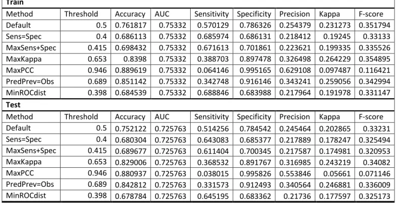
26 Considering a performance evaluation of a random forest in Kasko insurances (Table 5.2), it is possible to see how the measures are dependent on the probability’s threshold.

For example, considering the default threshold of 0.5, in the train, the precision is of 25.44%, but with a threshold that maximizes Kappa we can get a precision of 32.65%, reducing the sensitivity from 57.01% to 38.87%

Also, considering the different optimization criteria that define the threshold, it is possible to notice that the criterion that maximizes kappa’s measure allows a trade-off between sensitivity and precision values.

Moreover, accuracy values don’t give a true indication of the model’s usefulness. Considering the threshold that maximizes Kappa, the model has an accuracy of 83.98%, which may indicate that the model is performing well, but actually, considering the sensitivity of 38.87% and the precision of 32.65%, it is apparent that the churn prediction has complications.

In the lift (Table 5.3), as expected, it is possible to notice that the churn rate is bigger in the highest deciles and decreases monotonously in training, almost in the test (not in the deciles 8 and 9). The lift gives an idea about how much the churn rate is, with consideration to the average churn rate. Considering the lower deciles, after the 4th _{and 5}th _{for example, it is expected that the lift assumes a} value close to zero. The maximum value that the lift can have is when the churn rate is 100% in one decile, and all the policies are going to churn, in this case, the maximum lift is around 8.5, then, the lift 3.147, in the first decile, is compared with 8.5.

Figure 5.1 shows the distribution of the predicted probability by the real target. We expected that the area of the light curve is small in high probability, and peaks in low probability. The area of the dark curve is small in small probability and peaks in high probability, it is also better that these two curves are separated, lower is the misclassification error.

Table 5.2 Train and Test measures – RF in Kasko’s insurances

Train

Method Threshold Accuracy AUC Sensitivity Specificity Precision Kappa F-score Default 0.5 0.761817 0.75332 0.570129 0.786326 0.254379 0.231273 0.351794 Sens=Spec 0.4 0.686113 0.75332 0.685974 0.686131 0.218412 0.19245 0.33133 MaxSens+Spec 0.415 0.698432 0.75332 0.671613 0.701861 0.223621 0.199335 0.335526 MaxKappa 0.653 0.8398 0.75332 0.388703 0.897478 0.326498 0.264229 0.354895 MaxPCC 0.946 0.889619 0.75332 0.064146 0.995165 0.629108 0.097487 0.116421 PredPrev=Obs 0.689 0.851142 0.75332 0.342748 0.916146 0.343241 0.259056 0.342994 MinROCdist 0.398 0.684539 0.75332 0.688846 0.683988 0.217964 0.191978 0.331147 Test

Method Threshold Accuracy AUC Sensitivity Specificity Precision Kappa F-score Default 0.5 0.752122 0.725763 0.514256 0.784542 0.245464 0.202865 0.33231 Sens=Spec 0.4 0.680304 0.725763 0.643083 0.685377 0.217889 0.178247 0.325494 MaxSens+Spec 0.415 0.689677 0.725763 0.611404 0.700345 0.217587 0.174981 0.320953 MaxKappa 0.653 0.829006 0.725763 0.368532 0.891767 0.316985 0.243219 0.34082 MaxPCC 0.946 0.880937 0.725763 0.038015 0.995826 0.553846 0.05661 0.071146 PredPrev=Obs 0.689 0.842812 0.725763 0.331573 0.912493 0.340564 0.246881 0.336009 MinROCdist 0.398 0.678784 0.725763 0.645195 0.683362 0.21736 0.177597 0.325173

27

5.2.

P

In the following two pages, the results of the two universes are shown. In particular, only the models with highest AUC are shown and all the models are trained using under-sampling technique, because of that, they are an ensemble of 7 balanced samples models.

In compulsory motor insurance (Table 5.5), there is a model (Model RF+ANN1) that is an ensemble of two different models that are, in turn, an ensemble of the 7 balanced samples.

The probability’s threshold is defined using the Kappa’s optimization criterion, because, as shown previously, it stabilizes the values of precision and sensitivity.

All the binary classification measures are shown: in 2017 the evaluated set is the test. Table 5.3 Lift - RF in Kasko insurances

Train Test

Decil Churn Rate Lift Churn Rate Lift

1 36.300% 3.147 35.570% 3.084 2 19.924% 1.727 16.582% 1.438 3 15.163% 1.315 15.209% 1.319 4 11.273% 0.977 10.886% 0.944 5 9.656% 0.837 9.759% 0.846 6 7.709% 0.668 9.560% 0.829 7 5.694% 0.494 6.513% 0.565 8 3.905% 0.339 4.161% 0.361 9 3.850% 0.334 4.430% 0.384