Unconventional Regression for High-Dimensional Data Analysis

(1)

Unconventional Regression for High-Dimensional Data

Analysis

A DISSERTATION

SUBMITTED TO THE FACULTY OF THE GRADUATE SCHOOL OF THE UNIVERSITY OF MINNESOTA

BY

Yuwen Gu

IN PARTIAL FULFILLMENT OF THE REQUIREMENTS FOR THE DEGREE OF

DOCTOR OF PHILOSOPHY

Hui Zou, Adviser

(2)

(3)

A

CKNOWLEDGEMENTS

First and foremost, I would like to express my deepest gratitude to my advisor, Prof. Hui Zou, for his gracious support and encouragement over the past few years. His insights and vision have enlightened me in all aspects of statistical research and applications. I benefit so much from his sound knowledge in statistics, his wisdom and his professionalism. I feel extremely lucky to have Hui as my advisor.

My heartfelt gratitude also goes to the rest of my dissertation committee: Prof. Xiaoou Li, Prof. Wei Pan and Prof. Yuhong Yang. I thank them for their precious advice and insightful comments on my research. Meanwhile, I would like to give my sincere thanks to Prof. Galin Jones and Prof. Lan Wang for their support in my job search, to Yi Yang for all the insightful discussions, and to Boxiang Wang, Lan Liu, Bo Peng, Qi Yan, Gang Cheng, Qing Mai, Xin Zhang, Xiaoyi Zhu, Gongjun Xu, Zhihua Su and Jun Fan for their tremendous help in both research and life. I also thank all the other professors and graduate students in the School of Statistics for making my PhD life so enjoyable.

My special thanks are due to my parents, Jikang Gu and Fenlan Xu, for bringing me to the world in the first place and for supporting me mentally through every obstacle in my life.

Last but not least, this dissertation would not have been completed without my loving and supportive wife, Yanjia Yu.

(4)

D

EDICATION

To my parents and wife.

(5)

A

BSTRACT

Massive and complex data present new challenges that conventional sparse penalized mean regressions, such as the penalized least squares, cannot fully solve. For example, in high-dimensional data, non-constant variance, or heteroscedasticity, is commonly present but often receives little attention in penalized mean regressions. Heavy-tailedness is also frequently encountered in many high-dimensional scientific data. To resolve these issues, unconventional sparse regressions such as penalized quantile regression and penalized asymmetric least squares are the appropriate tools because they can infer the complete picture of the entire probability distribution.

Asymmetric least squares regression has wide applications in statistics, econometrics and finance. It is also an important tool in analyzing heteroscedasticity and is computationally friendlier than quantile regression. The existing work on asymmetric least squares only considers the traditional low dimension and large sample setting. We systematically study the Sparse Asymmetric LEast Squares (SALES) under high dimensionality and fully explore its theoretical and numerical properties. SALES may fail to tell which variables are important for the mean function and which variables are important for the scale/variance function, especially when there are variables that are important for both mean and scale. To that end, we further propose a COupled Sparse Asymmetric LEast Squares (COSALES) regression for calibrated heteroscedasticity analysis.

Penalized quantile regression has been shown to enjoy very good theoretical properties in the literature. However, the computational issue of penalized quantile regression has not yet been fully resolved in the literature. We introduce fast alternating direction method of multipliers (ADMM) algorithms for computing penalized quantile regression with the lasso, adaptive lasso, and folded concave penalties. The convergence properties of the proposed

(6)

iv

algorithms are established and numerical experiments demonstrate their computational efficiency and accuracy.

To efficiently estimate coefficients in high-dimensional linear models without prior knowledge of the error distributions, sparse penalized composite quantile regression (CQR) provides protection against significant efficiency decay regardless of the error distribution. We consider both lasso and folded concave penalized CQR and establish their theoretical properties under ultrahigh dimensionality. A unified efficient numerical algorithm based on ADMM is also proposed to solve the penalized CQR. Numerical studies demonstrate the superior performance of penalized CQR over penalized least squares under many error distributions.

(7)

List of Tables

2.1 Numerical summary of simulation results from the lasso, SCAD and MCP

penalized SALES regression for model (2.11):y Dx6Cx12Cx15Cx20C .0:7x1/". The sparsity recovery performance is measured by the selected active set size j OAj;the proportion pa of covering the true active set and the proportion p1 of selecting the signature variableX1: The estimation accuracy is measured by the L1 risk R1 and the L2 risk R2: The results are shown as averages over 100 replicates with standard errors listed in the parentheses when available . . . 20

2.2 Numerical summary of simulation results from the lasso, SCAD and MCP

penalized COSALES regression for model (2.11): y Dx6Cx12Cx15C

x20 C .0:7x1/". The selection accuracy is measured by the number of selected variablesj OA1jandj OA2j, and the proportionspa1andpa2of covering the true active sets. The estimation accuracy is measured by theL1 risks

R

1 andR

'

1;and theL2 risksR

2 andR

'

2:The results are shown as averages

over 100 replicates with standard errors listed in the parentheses. A fairly extreme-value ( D0:95) is used in the simulation for easy separation of the mean and scale . . . 30

(11)

LIST OF TABLES ix

2.3 Numerical summary of simulation results from the the lasso, SCAD and

MCP penalized COSALES regression for model (2.17): y Dx6Cx12C

x15Cx20C.0:7x1C0:7x12/". The selection accuracy is measured by the number of selected variables j OA1j and j OA2j, and the proportions pa1 and

pa2 of covering the true active sets. The estimation accuracy is measured by theL1 risksR

1 and R

'

1; and theL2 risksR

2 and R

'

2:The results are

shown as averages over 100 replicates with standard errors listed in the parentheses. A fairly extreme-value ( D0:95) is used in the simulation for easy separation of the mean and scale . . . 31 2.4 Analysis of microarray data reported inScheetz et al.(2006) using SALES

regressions with lasso, SCAD and MCP penalties. Three different values

of (0.3, 0.5 and 0.7) are used for each method. The number of active

variables selected using the whole data set is given in column 3. The average number of active variables selected and average predicted loss

.1=40/P

i2validation‰.yi ˇ0O x

T

iˇO/listed in columns 4 and 5 are calculated

from 50 random partitions of the original data with standard errors listed in parentheses . . . 33 2.5 Analysis of microarray data reported inScheetz et al.(2006) using

COS-ALES regressions with lasso, SCAD and MCP penalties. In this analysis,

D0:7is used. The number of active variables selected for the mean and scale using the whole data set is given in columns 2 and 3. The average num-ber of active variables selected for the mean and scale and average predicted loss.1=40/P i2validation‰0:5.yi 0O x T iO/C‰.yi 0O x T iO '0O x T i'O/

listed in columns 4 to 6 are calculated from 50 random partitions of the original data with standard errors listed in parentheses . . . 34

(12)

LIST OF TABLES x

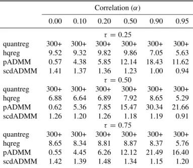
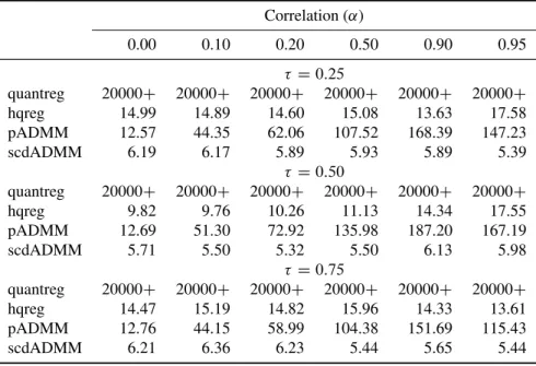
3.1 Timings (in seconds) for running lasso penalized quantile regression ( D 0:25; 0:5and0:75) on model (3.10) withnD100andp D1000over one hundredvalues. Timings reported are averaged over three runs. quantreg:

timing by the quantreg package (300+: above 300 seconds); hqreg:

timing by the hqregpackage; scdADMM and pADMM: timing by our

packageFHDQR. . . 67 3.2 Timings (in seconds) for running lasso penalized quantile regression ( D

0:25; 0:5and0:75) on model (3.10) withnD100andp D5000over one hundredvalues. Timings reported are averaged over three runs. quantreg:

timing by thequantregpackage (20000+: above 20000 seconds); hqreg:

packageFHDQR. . . 68 3.3 Timings (in seconds) for running lasso penalized quantile regression ( D

0:5and0:75) on model (3.11) withnD200andp D1000over one hun-dredvalues. All timings reported are averaged over three runs. quantreg:

timing by the quantreg package (400+: above 400 seconds); hqreg:

packageFHDQR.I: independent structure; AR0:5(AR0:8): autoregressive

structure with correlation0:5(0.8); CS0:5(CS0:8): compound symmetric

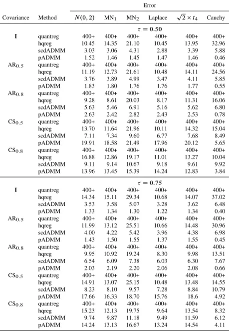
structure with correlation0:5(0:8). . . 69 3.4 Estimation and selection performance of the penalized least squares and

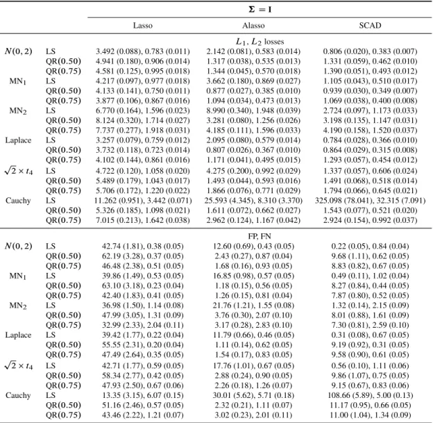
penalized quantile regression (with D0:5and0:75) for model (3.11) with independent covariates†DI. The estimation accuracy is measured by the

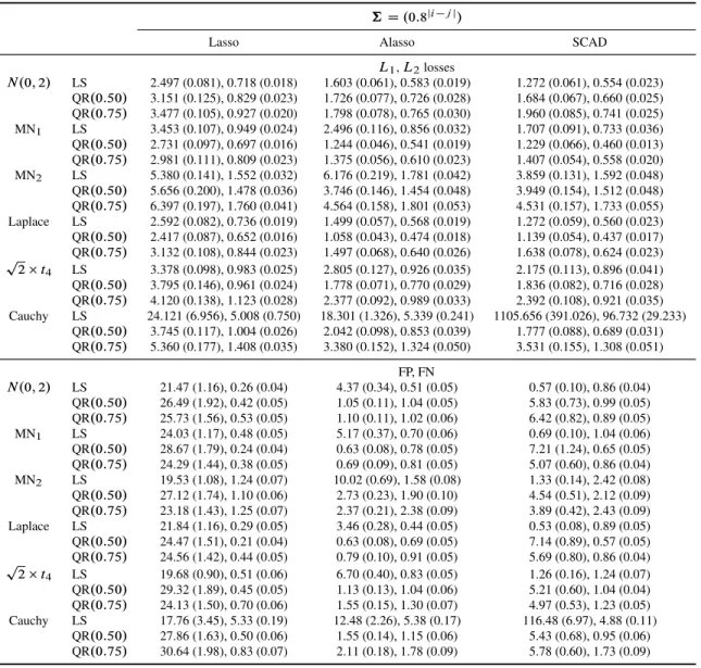
L1andL2losses and the selection accuracy is measured by the number of false positives (FP) and false negatives (FN). Numbers reported are averaged over 100 independent runs with their respective standard errors listed in the parentheses. . . 71

(13)

LIST OF TABLES xi

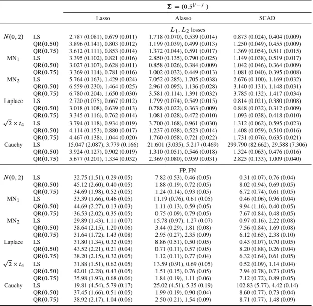
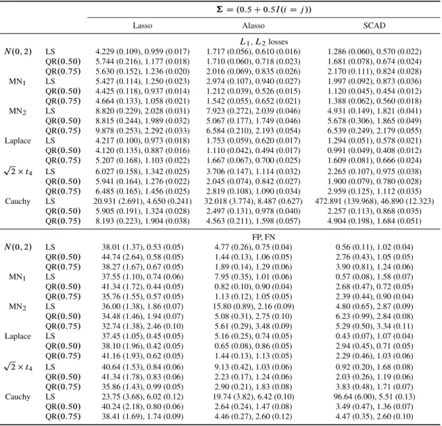
3.5 Estimation and selection performance of the penalized least squares and penalized quantile regression (with D0:5and0:75) for model (3.11) with covariance matrix† D .0:5ji jj/. The estimation accuracy is measured

by the L1 and L2 losses and the selection accuracy is measured by the

number of false positives (FP) and false negatives (FN). Numbers reported are averaged over 100 independent runs with their respective standard errors listed in the parentheses. . . 72 3.6 Estimation and selection performance of the penalized least squares and

penalized quantile regression (with D0:5and0:75) for model (3.11) with covariance matrix† D .0:8ji jj/. The estimation accuracy is measured

by the L1 and L2 losses and the selection accuracy is measured by the

number of false positives (FP) and false negatives (FN). Numbers reported are averaged over 100 independent runs with their respective standard errors listed in the parentheses. . . 73 3.7 Estimation and selection performance of the penalized least squares and

penalized quantile regression (with D0:5and0:75) for model (3.11) with covariance matrix† D.0:5C0:5I.i D j //. The estimation accuracy is measured by theL1andL2losses and the selection accuracy is measured by the number of false positives (FP) and false negatives (FN). Numbers re-ported are averaged over 100 independent runs with their respective standard errors listed in the parentheses. . . 74

(14)

LIST OF TABLES xii

3.8 Estimation and selection performance of the penalized least squares and penalized quantile regression (with D0:5and0:75) for model (3.11) with covariance matrix† D.0:8C0:2I.i D j //. The estimation accuracy is measured by theL1andL2losses and the selection accuracy is measured by the number of false positives (FP) and false negatives (FN). Numbers re-ported are averaged over 100 independent runs with their respective standard errors listed in the parentheses. . . 75 3.9 Timings (in seconds) for running lasso penalized quantile regression (with

D0:25; 0:50and0:75) on the microarray data reported inScheetz et al.

(2006) over one hundred values by quantreg (5000+: above 5000

seconds), scdADMM, pADMM and hqreg. All timings reported are

averaged over three runs. . . 77 3.10 Analysis of the microarray data reported inScheetz et al.(2006) by lasso

penalized quantile regression with the FHDQRpackage. The number of

genes selected and prediction errors are averaged over 50 runs for the random partition columns. Numbers in the parentheses are standard errors of their corresponding averages. . . 77

4.1 Simulation results for model (4.10) with n D 100; p D 600 and † D

.0:5ji jj/: Numbers listed are averages over 100 independent runs, with standard errors reported in the parentheses . . . 96

(15)

LIST OF TABLES xiii

.0:8ji jj/: Numbers listed are averages over 100 independent runs, with standard errors reported in the parentheses . . . 99 B.1 Timings (in seconds) for running lasso penalized quantile regression ( D

0:25) on Friedman’s model (˛ D 0:5; n D 100 and p D 200) over a

sequence of pre-chosenvalues byMM,quantregandADMM . . . 154

B.2 Timings (in seconds) for running lasso penalized quantile regression ( D

0:75) on Friedman’s model (˛ D 0:5; n D 100 and p D 400) over a

sequence of pre-chosenvalues byADMM,hqreg,QICDandquantreg.

The question mark implies inaccurate result . . . 156 C.1 Timings (in seconds) for running lasso penalized CQR over a sequence

of one hundred values on simulated data from model (4.10) using the

(16)

List of Figures

B.1 Objective function values of lasso penalized quantile regression ( D0:75)

fitted on model (3.10) with ˛ D 0:5, n D 100; and p D 5000 at the

optimal solutions computed by quantreg, scdADMM, pADMM and

hqregalong a sequence of one hundred pre-chosenvalues. . . 151 B.2 Objective function values of lasso penalized quantile regression ( D0:25)

fitted on Friedman’s model (˛ D 0:5; n D 100and p D 200) with MM,

quantregand ADMM along a sequence of pre-chosenvalues. . . 154 B.3 Objective function values of lasso penalized quantile regression ( D0:75)

fitted on Friedman’s model (˛ D 0:5; nD 100andp D400) withADMM,

quantreg,QICD, andhqregalong a sequence of pre-chosenvalues. . 155

(17)

Chapter 1

Introduction

1.1 Background

Our decade has seen a surge of massive and complex data due to the advance of data acquisition technologies. As an integral part of the “big data” revolution, high-dimensional data are more and more frequently collected in a wide variety of fields, such as biomedical sciences, finance, climate studies, astronomy and neuroscience. These high-dimensional data pose many challenges both theoretically and numerically. This urges the development of new methodologies and tools to analyze high-dimensional data.

It is well known that in the high-dimensional regime, traditional statistical analyses break down when the number of unknown parameters exceeds the number of observations (“largepsmalln”) due to the “curse of dimensionality” (Donoho et al.,2000). Therefore, to solve high-dimensional problems, many methods have been proposed to reduce the dimensionality, usually by imposing some type of low-dimensional constraints on the model space. Exemplary approaches include the penalized regression with various sparsity constraints on the coefficients, matrix estimation with low-rank assumptions, covariance or precision matrix estimation with structure sparsity patterns, and so on. In all these examples, the regularization idea proves to be very successful. To that end, for the sparse penalized regression alone, various regularization techniques have been proposed to control the model

(18)

1.2. DISSERTATIONOUTLINE 2

complexity and to achieve intended sparsity structures. Popular regularization methods include the lasso (Tibshirani,1996), SCAD (Fan and Li,2001), elastic net (Zou and Hastie,

2005), adaptive lasso (Zou,2006), Dantzig selector (Candes and Tao,2007), MCP (Zhang,

2010), and so on. Under such regularization, the penalized least squares regression has received tremendous attention in applications and has been widely adopted in practice to analyze high-dimensional data with a huge number of variables due to its nice theoretical guarantees and computational efficiency.

In the penalized least squares regression, the variance function is often assumed constant for theoretical convenience. However, in high-dimensional data, non-constant variance, or heteroscedasticity, is commonly present. Studies on expression quantitative trait locus (eQTL) confirmed the existence of heteroscedasticity in lots of high-dimensional data (Wang et al.,2012;Daye et al.,2012). Moreover, high-dimensional data subject to heavy-tailed errors are also commonly encountered in various scientific fields. For such data, conventional sparse penalized mean regressions, such as the penalized least squares, will encounter problems. To resolve these issues, unconventional sparse penalized regressions, such as the penalized quantile regression and penalized Huber regression, are the appropriate tools. In this dissertation, we systematically study a new type of unconventional sparse penalized regression, namely, the penalized asymmetric least squares regression, and its variant to deal with heteroscedasticity in high-dimensional data. We also discuss the computational issues of the penalized quantile regression. In terms of coefficient estimation in a linear model, we study the penalized composite quantile regression as a safe procedure for efficient coefficient estimation.

1.2 Dissertation Outline

The dissertation is mainly composed of three chapters (Chapters 2 – 4), which discuss three different types of unconventional regressions in the high-dimensional setting. The main

(19)

1.2. DISSERTATIONOUTLINE 3

goal of this dissertation is to provide good methodologies and practical tools to deal with high-dimensional data that exhibit heteroscedasticity and heavy-tailedness.

In Chapter 2, we introduce the sparse asymmetric least squares and demonstrate its potential in dealing with heteroscedasticity in high-dimensional data. We establish the theoretical properties of both lasso and folded concave penalized asymmetric least squares. A unified numerical algorithm is proposed to solve penalized asymmetric least squares with various penalties. For more calibrated analysis of heteroscedasticity, we propose a coupled sparse asymmetric least squares regression and study both its theoretical and numerical properties.

In Chapter 3, we propose efficient alternating direction method of multipliers (ADMM) algorithms for numerically solving the penalized quantile regression with various penalties. We show the convergence properties of our proposed algorithms. Computational efficiency and accuracy of the proposed algorithms are demonstrated through extensive numerical studies.

In the context of estimating coefficients in a linear model, we study the penalized composite quantile regression in Chapter 4 under ultrahigh dimensionality. Composite quantile regression is known to be a safe alternative to quantile regression in providing high efficiency in coefficient estimation. We consider both lasso and folded concave penalized composite quantile regression and study their theoretical properties. Since the objective function is highly non-smooth, the penalized composite quantile regression poses great challenges in optimization. We propose a sparse coordinate descent ADMM algorithm for efficiently solving the penalized composite quantile regression. We demonstrate the superior finite sample performance of the penalized composite quantile regression over the penalized least squares regression under many error distributions in numerical studies.

Finally, we conclude the dissertation in Chapter 5, with a brief discussion of some potential future work.

(20)

Chapter 2

High-Dimensional Generalizations of

Asymmetric Least Squares Regression

and Their Applications

Asymmetric least squares regression is an important method that has wide applications in statistics, econometrics and finance. The existing work on asymmetric least squares only considers the traditional low dimension and large sample setting. In this chapter, we systematically study the Sparse Asymmetric LEast Squares (SALES) regression under high dimensions where the penalty functions include the lasso and nonconvex penalties. We develop a unified efficient algorithm for fitting SALES and establish its theoretical properties. As an important application, SALES is used to detect heteroscedasticity in high-dimensional data. Another method for detecting heteroscedasticity is the sparse quantile regression. However, both SALES and the sparse quantile regression may fail to tell which variables are important for the conditional mean and which variables are important for the conditional scale/variance, especially when there are variables that are important for both the mean and the scale. To that end, we further propose a COupled Sparse Asymmetric LEast Squares (COSALES) regression which can be efficiently solved by an algorithm similar to that for solving SALES. We establish theoretical properties of COSALES. In particular, COSALES using the SCAD penalty or MCP is shown to consistently identify the two important subsets for the mean and scale simultaneously, even when the two subsets overlap. We demonstrate

(21)

2.1. INTRODUCTION 5

the empirical performance of SALES and COSALES by simulated and real data.

2.1 Introduction

High-dimensional data have received tremendous attention in the last decade due to the advance of data collection technology. Sparse estimation, which uses penalization or regular-ization techniques to perform variable selection and estimation simultaneously, has become a mainstream approach for analyzing high-dimensional data. Popular penalized estimators include theL1-type selectors such as the lasso (Tibshirani,1996) and Dantzig (Candes and Tao,2007) selectors and the nonconvex penalized estimators such as the SCAD (Fan and Li,2001) and MCP (Zhang,2010) estimators. Some embrace theL1-regularization for its computational efficiency, while others prefer to use the nonconvex penalization due to its oracle (Fan and Li,2001) property.

The current literature on sparse estimation often assumes homoscedasticity. For example, the existing theory for the sparse linear regression model is based on the classical linear model assumption in which the mean function is linear and the errors are i.i.d. with zero mean and constant variance. The heteroscedasticity issue is often overlooked for theoretical convenience. However, heteroscedasticity often exists due to heterogeneity in measurement units or accumulation of outlying observations from numerous sources of inputs. This is particularly relevant with high-dimensional data. For example, in genomics experiments, tens of thousands of genes are often analyzed simultaneously by microarrays and occasional outlying measurements appearing in numerous experimental and data-preprocessing steps can accumulate to form heteroscedasticity in the data obtained therein. These data sets are often of high dimension since only a small number of subjects are available for the study. Several studies on expression quantitative trait loci (eQTLs) (Wang et al.,2012;Daye et al.,2012) confirmed the presence of heteroscedasticity in these high-dimensional data and it was shown that genetic variants have effects on both the mean and the scale (i.e.,

(22)

2.1. INTRODUCTION 6

standard deviation) of gene expression levels. In such scenarios, it is important to incorporate heteroscedasticity to make inference from the limited amount of data. To our knowledge, most existing work on high-dimensional data analysis fails to address the heteroscedasticity issue.

The sparse quantile regression was proposed inWang et al.(2012) to detect heteroscedas-ticity in high-dimensional data. Quantile regression (Koenker and Bassett,1978) is appro-priate under heteroscedasticity, because it uses an asymmetric absolute value loss. The key word is “asymmetric,” not the absolute value loss. The absolute value loss is computa-tionally more challenging than the squared error loss. Computational efficiency is always one of the primary considerations in high-dimensional data analysis. This motivates us to study the asymmetric least squares (ALS) regression under high dimensionality. The ALS regression has been studied inEfron(1991). It is also known as the expectile regression in econometrics and finance. SeeNewey and Powell (1987);Taylor (2008); Kuan et al.

(2009);Xie et al.(2014). The key idea in ALS is to assign different squared error loss to the positive and negative residuals, respectively. By doing so, one can infer a more complete description of the conditional distribution than ordinary least squares (OLS). Thus, ALS and quantile regression share a common virtue although they differ technically. The most notable advantage of ALS over quantile regression is that the former employs a smooth differentiable loss, which considerably alleviates the computational effort involved and also makes the theoretical analysis more amenable. These two are desirable properties under high dimensionality.

In this chapter, we develop the methodology and theory for the Sparse Asymmetric LEast Squares (SALES) regression and show its applications in detecting heteroscedasticity in a general class of sparse models in which the set of relevant covariates may vary from segment to segment on the conditional distribution. For the nonconvex penalized SALES regression, we prove its strong oracle property. We then discuss an important issue overlooked by existing methods dealing with heteroscedasticity in high dimensional data, that is, how to

(23)

2.2. HIGH-DIMENSIONALSALES REGRESSION 7

exactly differentiate the sets of relevant covariates for the mean and scale when they have overlaps. To resolve this issue, we propose a novel COupled Sparse Asymmetric LEast Squares (COSALES) regression method to select important variables for the mean and scale of the conditional distribution simultaneously. The strong oracle property is also shown for the nonconvex penalized COSALES estimator. We develop novel efficient algorithms for computing both SALES and COSALES.

The remainder of the chapter is organized as follows. We study SALES in Section 2.2 and demonstrate its application in detecting heteroscedasticity in Section 2.3. In Section 2.4, we introduce and study COSALES. The performance of COSALES is illustrated by two simulation examples. In Section 2.5, we apply SALES and COSALES to analyze a real microarray dataset. The proofs of all main theoretical results are relegated to Section 2.6.

2.2 High-Dimensional SALES Regression

2.2.1 Background and setup

We start by defining the-mean of a random variableZ 2R;

E

.Z/arg min

a2R

Ef‰.Z a/g; 2.0; 1/; (2.1)

where‰.u/D j I.u < 0/ju2is the asymmetric squared error loss (see e.g.Newey and Powell,1987;Efron,1991) andI./represents the indicator function. Similar definition can be found inEfron(1991). As a matter of fact, our-mean corresponds to Efron’sw-mean,

wherew D =.1 /. Hereafter, we callE the asymmetric expectation operator (with

asymmetry coefficient). Note thatE0:5coincides with the usual expectation operator_E. The-mean is also called the-expectile in the econometrics literature (Newey and Powell,

1987). By varying;the-mean quantifies different “locations” of a distribution, and thus it can be viewed as a generalization of the mean and an alternative measure of “location” of a

(24)

distribution.

The asymmetric squared error loss‰./gives rise to the ALS regression, in which the squared error loss is given different weights depending on whether the residual is positive or negative. LetXD.X1; : : : ; Xp/be thenp design matrix withXj D.x1j; : : : ; xnj/T_; j D 1; : : : ; p; andy D .y1; : : : ; yn/T

be then-dimensional response vector. The design matrix may also be written asXD.x1; : : : ;xn/T_;_where_x

i D.xi1: : : ; xip/T; i D1; : : : ; n:

The ALS regression is done via

bˇALS Darg min

ˇ2Rp n X iD1 ‰.yi xT iˇ/:

When D0:5;the ALS regression reduces to the OLS regression. When ¤0:5, due to

the asymmetric nature and relative smoothness of‰./, the ALS regression provides a con-venient and computationally efficient way of summarizing the conditional distribution of a response variable given the covariates (Newey and Powell,1987;Efron,1991). Applications of the ALS regression include estimation of the value at risk and expected shortfall (Taylor,

2008;Kuan et al.,2009), medical baseline correction (Eilers and Boelens,2005), and small area estimation (Chambers and Tzavidis,2006;Salvati et al.,2012) among others.

In the literature, the underlying model considered for studying the theoretical property of the ALS regression is

yDXˇC"; (2.2) where ˇ is a p-dimensional vector of unknown parameters and " is the vector of n

independent errors, which satisfy E."_ijxi/ D 0; i D 1; : : : ; n for some 2 .0; 1/: It

follows thatE.yijxi/D xT_iˇ;which means that the conditional-mean ofyi is a linear

combination ofxi; i D 1; : : : ; n:A similar model to (2.2) was considered inWang et al.

(25)

modeled as a linear combination of the covariates. In model (2.2), it is important to realize that the coefficient vectorˇ is allowed to change with;which makes modeling for different “locations” of the conditional distribution possible, and as a result heteroscedasticity in the data, when it exists, can be inspected by this model. For convenience, we will drop the superscript forˇ and" when no confusion arises.

To accommodate high-dimensional data in model (2.2), we allow the number of covari-atespto increase with the sample sizen;and moreover, we are primarily interested in cases wherep exceedsn(p > n). We adopt the sparsity assumption that only a small number of covariates contribute to the response. Suppose ˇ D .ˇ₁; : : : ; ˇ_p/T

is the parameter vector of the true underlying model that generates the data and assumeˇiss-sparse, where

s D jAjwithAsupp.ˇ/D fjWˇ_j ¤0g:

2.2.2 Methodology

To select important variables and estimateˇin model (2.2) when the dimension is high, let us consider the following penalized SALES regression:

min ˇ2Rp n 1 n X iD1 ‰.yi xT iˇ/C p X jD1 p.ˇj/; (2.3)

where‰./is the asymmetric squared error loss andp./is a nonnegative penalty function with regularization parameter2.0;1/. In the remainder of this chapter, we mainly focus on the lasso and nonconvex penalties.

L1-penalized SALES regression

For ease of notation, let Ln.ˇ/ D n 1Pn

iD1‰.yi xTiˇ/: The L1-penalized SALES

(26)

2.2. HIGH-DIMENSIONALSALES REGRESSION 10 problem min ˇ2Rp Ln.ˇ/Classo p X jD1 jˇjj; lasso 2.0;1/: (2.4)

This is to take p.u/D jujin (2.3). The lasso is computationally attractive and can be solved by efficient algorithms such as the LARS (Efron et al.,2004), the coordinate descent method (Friedman et al.,2010) and the generalized coordinate descent algorithm (Yang and Zou,2013).

For efficient computation ofbˇlasso in (2.4), we propose an algorithm called SALES

which combines the cyclic coordinate descent (Tseng,2001) and proximal gradient algo-rithms (Parikh and Boyd,2013). Our algorithm solves the following more general “weighted”

L1-minimization problem: min ˇ2Rp Ln.ˇ/C p X jD1 wjjˇjj (2.5)

with constantswj 0for allj:Our consideration of formulation (2.5) is twofold. First, it not only can be directly applied to the SALES lasso problem (2.4) by settingwj Dlassofor allj,

but also can be used to solve the convex approximations to the nonconvex penalized SALES estimation (see step (a) of Algorithm 2). Second, leaving some coefficients unpenalized is simply a matter of setting their corresponding weights to zero. Doing so gives us the flexibility to decide which covariates should always be kept in the model. The algorithm is described as follows.

ForvD.v1; : : : ; vd/T ₂

Rd;denotev k D.v1; : : : ; vk 1; vkC1; : : : ; vd/Tthe subvector

ofvwith itskth component removed. Recovervfromv k by writingvD Œvk;v k:Let

ˇr D.ˇr

(27)

algorithm. For ease of notation, denote

brC_k1 D.ˇr1C1; : : : ; ˇ rC1 k 1; ˇ r kC1; : : : ; ˇ r p/ T ; 1kp; r 0:

Applying the coordinate descent method, to updateˇk in the.r C1/th cycle, we solve the following minimization problem:

min ˇk2R `n.ˇkIbrC_k1/Cwkjˇkj; (2.6) where`n.ˇkIbrC_k1/DLn.Œˇk;brC_k1/Dn 1Pn iD1‰.yi xTi; kb rC1 k xi kˇk/:One can show that`0n.ˇkIb rC1

k /is Lipschitz continuous with constantLk D2cnN 1

kXkk22;where k k2is the Euclidean norm. Thus, the proximal gradient method can be employed to solve problem (2.6) ˇ_kr;0 WDˇ_kr; ˇ_kr;sC1 WDSL_k1wk.ˇ r;s k L 1 k `0n.ˇ r;s k Ib rC1 k //; s0; (2.7)

where_Sv.u/Dsgn.u/.juj v/Cdenotes the soft thresholding operator withuC DuI.u > 0/:We let (2.7) run fors_kr iterations and setˇ_krC1 WDˇr;s

r k

k :Our algorithm is summarized in

Algorithm 1. We prove in Appendix A that Algorithm 1 converges at least linearly.

Nonconvex penalized SALES regression

Nonconvex penalties have been used in a broad type of sparse regression models (Fan and Lv,2011;Wang et al., 2013; Fan et al.,2014b). The most popular nonconvex penalties include the smoothly clipped absolute deviation (SCAD) penalty (Fan and Li,2001) and the minimax concave penalty (MCP,Zhang,2010). For some constant > 2;the SCAD

(28)

Algorithm 1:SALES — Cyclic coordinate descent plus proximal gradient algorithm for solving the weightedL1-minimization problem (2.5)

1. Initialize the algorithm withˇ0_D.ˇ₁0; : : : ; ˇ0_p/T_: 2. ForrD0; 1; 2; : : : ; m 1; (2.1) ForkD1; : : : ; p; (2.1.1) Initializeˇr;0_k WDˇ_kr: (2.1.2) ForsD0; 1; 2; : : : ; sr_k 1; (2.1.2.1) Calculateˇr;s_k C1WDSL 1 k wk.ˇk L 1 k `0n.ˇ r;s k Ib rC1 k //. (2.1.3) Setˇr_kC1 WDˇr;s r k k : (2.2) SetˇrC1_WD.ˇ₁rC1; : : : ; ˇ_prC1/T_: 3. Outputbˇ WDˇ m_: penalty is given by p.u/DjujI.juj /C juj . juj/ 2 2. 1/ I. <juj / C. C1/ 2 2 I.juj> /: (2.8)

The use of D 3:7for the SCAD penalty is recommended inFan and Li(2001) from a

Bayesian perspective. The MCP is characterized by

p.u/D juj u 2 2 I.juj /C 2 2 I.juj > / (2.9)

for some > 1:The use of D2is suggested inZhang(2010). In this chapter, we consider both SCAD and MCP penalized SALES regression.

The main motivation for using the nonconvex penalties is to achieve the oracle property. For the SALES regression, the oracle estimator is

bˇoracle D arg min

ˇ2RpWˇAcD0

(29)

In practice, the oracle estimator is infeasible, but it sets a benchmark for evaluation of other estimators. Many papers have shown that the nonconvex penalized least squares can find the oracle estimator with high probability (Wang et al.,2013;Fan et al.,2014b). In particular,

Fan et al.(2014b) showed that the local linear approximation (LLA) algorithm (Zou and Li,

2008) converges to the oracle estimator under regularity conditions. The LLA algorithm fits a sequence of weightedL1-regularization problems. Since we already have Algorithm 1 for computing any weightedL1-penalized SALES regression, we adopt the LLA algorithm for solving the nonconvex penalized SALES estimation problem (2.3). The details of the LLA algorithm are shown in Algorithm 2. Note that step (a) can be readily solved by Algorithm 1.

Algorithm 2:Local linear approximation (LLA) algorithm for solving the nonconvex penalized SALES estimation problem (2.3)

1. Initializebˇ

0

WDbˇ

initial_:_{Compute weights}

O

w_j0Dp0.j Oˇ0_jj/; j D1; : : : ; p:

2. FormD1; 2; : : : ;repeat the LLA iteration in (a) and (b) until convergence (a) Solve the following convex optimization problem forbˇm

bˇ m WDarg min ˇ2Rp Ln.ˇ/C p X jD1 O wm 1_j jˇjj:

(b) Update the weightswO_jmDp0.j Oˇ_jmj/; j D1; : : : ; p:

In our numerical examples, we tried using both the SALES lasso estimator and zero as the initial values of the LLA algorithm for computing the nonconvex penalized SALES estimator. Our practice is based on theoretical results in Section 2.2.3.

2.2.3 Theory

In this section, we theoretically analyze the SALES regression. We consider the case where the covariates are from a fixed design.

The following notation will be used. For any vector v D .v1; : : : ; vp/T ₂

(30)

arbitrary index set I f1; : : : ; pg; we write vI D .vj; j 2 I /T and denote by XI D .xj; j 2 I /the submatrix consisting of the columns ofXwith indices inI:The complement

ofI is denoted byIc _{D f}_{1; : : : ; p}_gn_I:_For_q ₂_Œ1;₁_;_the_Lq_{-norm of}_v_{is denoted by}_k_v_kq:

Sub-Gaussian norm (Rudelson and Vershynin,2013) of a random variableZis denoted by

kZkSG Dsupk1k 1=2.EjZjk/1=k:Leta_b Dmax.a; b/anda^b Dmin.a; b/for real

numbersaandb:For a differentiable functionf WRp !R;we writerf .v/D@f .v/=@v andrIf .v/D.@f .v/=@vj; j 2 I /T_:

We usemin./andmax./to represent respectively

the smallest and largest eigenvalues of a symmetric matrix. We also letcD ^.1 /and

N

c D_.1 /:

L1-penalized SALES regression

The estimation accuracy of the lasso has been extensively studied in the literature; see, for example,Negahban et al.(2012) andYe and Zhang(2010). LetC D fı 2 RpW kıAck1 3kıAk1 ¤ 0g be a cone in_Rp:Let min D min.n 1XTAXA/andmax D max.n 1XTAXA/:

We assumemin> 0so that the important variables are not linearly dependent. To study the

estimation accuracy of the SALES lasso, we impose the following conditions on the design matrixXand the random errors":

(C1) The columns ofXare normalizable, that is,M0Dmax1jp k Xjk2

p

n 2.0;1/:

(C2) The random errors"i are i.i.d. sub-Gaussian random variables satisfyingE."i/D 0; i D1; : : : ; n. (C3) Dinfı2C kXık 2 2 nkık22 2 .0;1/: (C4) %Dinfı2C kXık 2 2 nkıAk1kık1 2.0;1/:

Condition (C3) is called the restricted eigenvalue condition and has been frequently assumed in the literature to study the lasso and Dantzig selectors. See Bickel et al.

(31)

(2009), Meier et al. (2009), and Negahban et al. (2012). Condition (C4), the general-ized invertability factor (GIF) condition, is closely related to condition (C3) and has also been often adopted to study the lasso and Dantzig selectors. See discussion of these condi-tions inYe and Zhang(2010) andHuang and Zhang(2012). Both conditions (C3) and (C4) are crucial assumptions to establish estimation consistency of the lasso for high-dimensional data.

Theorem 2.1

Suppose in model (2.2) the true coefficientsˇares-sparse and assume conditions (C1-C2) hold. Letbˇlasso be any optimal solution to the SALES lasso problem (2.4). Then with

probability at least1 pALS

1 ;kbˇlasso ˇk23s1=2lasso.4c/ 1if condition (C3) holds,

andkbˇlasso ˇk₁ 3_lasso.4%c/ 1if condition (C4) holds, where

p1ALSD2pexp _{C n}2 lasso 4K02M02 ;

K0 D k‰0."i/kSG with ‰0./ being the derivative of ‰./; and C > 0 is an absolute

constant.

Remark 2.1 In some applications, it is natural to leave a given subset of the parameters unpenalized in the penalized framework (2.3). LetRdenote the index set of such parameters. For example, when X1 is a vector consisting of all ones, R D f1g reflects the common practice of leaving the intercept term not penalized. In this case, it is natural to modify the penalized SALES estimation problem (2.3) to be

min

ˇ2Rp

Ln.ˇ/C X j2Rc

p.ˇj/:

With lasso penalty, the SALES algorithm can be readily used to solve the above case. Moreover, similar theoretical analysis can be carried out with slight modifications. For

(32)

instance, in the SALES lasso problem (2.4) we can define A0 supp.ˇ_Rc/ and C0 D

fı 2RpW kı.A0_[_R/ck1 3kı_A0_[_Rk1¤0g:Conditions (C3) and (C4) can be then modified

respectively as 0D inf ı2C0 kXık22 nkık2 2 2.0;1/ and %0D inf ı2C0 kXık22 nkıA0_[_Rk1kık₁ 2 .0;1/:

To establish the selection consistency of the lasso, it is almost necessary to impose the irrepresentable condition; seeZou (2006) andZhao and Yu (2006). When the focus is on identifying the underlying sparsity pattern, the nonconvex penalized regression is a competitive alternative as it requires weaker conditions to achieve selection consistency.

Nonconvex penalized SALES regression

To offer a unified treatment of the SCAD and MCP penalized SALES regression, our theoretical analysis handles the following class of nonconvex penalties:

(P1) p.u/Dp. u/I

(P2) p.u/is nondecreasing and concave inu 2Œ0;1/andp.0/D0I

(P3) p.u/is differentiable inu2.0;1/I

(P4) p0.u/a1foru2 .0; a2andp0.0/ WDp0.0C/a1I

(P5) p0.u/D0foru2Œa;1/with some prespecified constanta > a2;

wherea1 and a2 are fixed constants characteristic of the penalty functions. It is easy to verify that both the SCAD penalty and MCP are in the above class.

We show that the sparse solutions obtained by the LLA algorithm in Section 2.2.2 possess the oracle property. Assume sufficient signal strength in the nonzero components of

(33)

(A1) minj2Ajˇjj> .aC1/:

Theorem 2.2

Suppose in model (2.2) the true coefficientsˇares-sparse and satisfy assumption (A1). Assume conditions (C1-C2) hold and takebˇlasso as the initial value. Leta0 D1^a2:Take

3s1=2

lasso.4a0c/ 1when (C3) holds, or take3lasso.4a0%c/ 1 when (C4) holds,

or takeŒ3s1=2lasso.4a0c/ 1^Œ3lasso.4a0%c/ 1when both (C3) and (C4) hold. The

LLA algorithm (Algorithm 2) converges tobˇoracle after two iterations with probability at

least1 pALS

1 pALS2 p3ALS;wherep ALS 1 is given in Theorem 2.1, pALS 2 D2.p s/exp C a21n2 4K2 0M02 C.Q1In; s; K0; M0; max; 0/ and pALS 3 D.2cminRIn; s; K0; M0; max; 0/;

where Q1 D a1cmin 2cN max1=2M0

1

; 0 D var.‰0."i//; R D minj2Ajˇjj a; K0 is

defined in Theorem 2.1 and./is a function defined by

.xIn; s; K; M; ; /D2sexp C nx2 K2_M2_s ^2exp _C2_Œ.n1=2_x 1=2_s1=2_/C2 K4 ;

andC > 0is an absolute constant.

It is interesting to note that with the SCAD penalty or MCP, a three-step LLA algorithm starting from the zero vector may also work. Indeed, for these two penalties we have

p0.0/D;so if we can takeDlasso;this would give us the SALES lasso estimator in

(34)

2.3. APPLICATION OFSALES: DETECTING HETEROSCEDASTICITY 18

Corollary 2.1

Assume the same framework of Theorem 2.2 and suppose the SCAD penalty (2.8) or MCP (2.9) is used. If condition (C3) holds and4a0c 3s1=2, or if condition (C4) holds and4a0%c3, or if both (C3) and (C4) hold andŒ3s1=2./ 1^Œ3.%/ 14a0c, the LLA algorithm (Algorithm 2) initialized by zero converges to the oracle estimator after three iterations with probability at least1 2pexpf C n2.4K₀2M₀2/ 1g pALS

2 p3ALS;where pALS

2 andp2ALSare given in Theorem 2.2.

2.3 Application of SALES: Detecting Heteroscedasticity

Due to asymmetry of the squared error loss, the SALES regression (2.3) can be employed to detect heteroscedasticity in high-dimensional data. In the following, we use a simulation example to illustrate this application. For the nonconvex penalty functions used in the simulation, we fix D3:7for the SCAD penalty (2.8) and D2for the MCP (2.9).

EXAMPLE1. We adopt a model fromWang et al.(2012). In the model, the covariates are generated in two steps. First, we generate copies of.z1; : : : ; zp/T_{from the multivariate}

normal distributionN.0;†/ with† D .0:5ji jj/pp:In the second step, for each copy

of.z1; : : : ; zp/T_;_{we set}_x1 _D _ˆ.z1/_and _xj _D _zj _for_j _D _{2; 3; : : : ; p;}_where_ˆ./_{is the}

standard normal CDF. The response is then simulated from the following normal linear heteroscedastic model:

y Dx6Cx12Cx15Cx20C.0:7x1/"; (2.11)

where"N.0; 1/is independent of the covariates. This model was considered inWang et al.(2012) for the sparse quantile regression, where a sample sizenD300and covariate

dimensions p D 400 and 600 were considered. We apply the SALES regression (2.3)

(35)

2.3. APPLICATION OFSALES: DETECTING HETEROSCEDASTICITY 19

of demonstration, we choosen D300and p D600:A validation set of sizen D 300is generated independently to tune the regularization parameter by minimizing the validation

errorP

i2validation‰.yi x

T

ibˇ/for the computed estimatebˇ;where D0:5and0:85are

considered.

For comparison purpose, we included in this simulation the SALES lasso (2.4) and two variations of the LLA algorithm for each nonconvex penalized SALES regression: the two-step LLA algorithm initialized by the lasso estimator (SCAD, MCP), and the three-step LLA algorithm initialized by zero (SCAD0, MCP0).

Letbˇbe the coefficient estimates from a given method. Based on 100 replicates, the

following measurements are calculated to evaluate the sparsity recovery and estimation performance of that method:

j OAj W the average size of the active setAOD fjW Oˇj ¤0gofbˇ:

pa W proportion of the event A OA; where Ais the active set of ˇ. When D 0:5;

AD f6; 12; 15; 20gand when ¤0:5; AD f1; 6; 12; 15; 20g: p1W proportion of the event thatf1g OA:

R1W the averageL1riskkbˇ ˇk1:

R2W the averageL2riskkbˇ ˇk2:

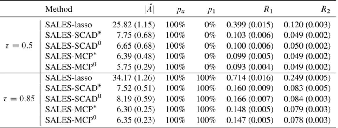
The simulation results are shown in Table 2.1. The following conclusions can be made: (1) The variablex1 in the scale function is often not recovered by penalized least-squares

( D0:5). However, when several-means (e.g., D0:85) are inspected together, it is possible to detect this variable with high probability. This shows that indeed the SALES regression can be used to detect heteroscedasticity.

(2) Compared to the SALES lasso, the nonconvex penalized SALES regression selects much fewer irrelevant covariates and has better estimation accuracy.

(36)

2.4. HIGH-DIMENSIONALCOSALES REGRESSION 20

(3) The three-step LLA algorithm starting from zero produces similar results to the two-step LLA algorithm starting from the lasso solution.

Table 2.1: Numerical summary of simulation results from the lasso, SCAD and MCP penalized SALES regression for model (2.11):y Dx6Cx12Cx15Cx20C.0:7x1/". The sparsity recovery performance is measured by the selected active set sizej OAj;the proportion

pa of covering the true active set and the proportionp1of selecting the signature variable

X1:The estimation accuracy is measured by theL1riskR1and theL2riskR2:The results are shown as averages over 100 replicates with standard errors listed in the parentheses when available Method j OAj pa p1 R1 R2 D0:5 SALES-lasso 25.82 (1.15) 100% 0% 0.399 (0.015) 0.120 (0.003) SALES-SCAD 7.75 (0.68) 100% 0% 0.103 (0.006) 0.049 (0.002) SALES-SCAD0 6.65 (0.68) 100% 0% 0.100 (0.006) 0.050 (0.002) SALES-MCP 6.39 (0.48) 100% 0% 0.099 (0.005) 0.049 (0.002) SALES-MCP0 5.75 (0.29) 100% 0% 0.093 (0.004) 0.049 (0.002) D0:85 SALES-lasso 34.17 (1.26) 100% 100% 0.714 (0.016) 0.249 (0.005) SALES-SCAD 7.52 (0.51) 100% 100% 0.160 (0.009) 0.083 (0.005) SALES-SCAD0 8.19 (0.59) 100% 100% 0.166 (0.007) 0.084 (0.003) SALES-MCP 6.30 (0.25) 100% 100% 0.148 (0.005) 0.079 (0.003) SALES-MCP0 6.35 (0.23) 100% 100% 0.147 (0.005) 0.078 (0.003)

2.4 High-Dimensional COSALES Regression

In Section 2.3, we showed that the SALES regression provides a means of detecting het-eroscedasticity in high-dimensional data. Indeed, in the linear heteroscedastic model (2.11), the signature variablex1;which appears in the scale function, was detected through com-parison of different-means. However, in high-dimensional heteroscedastic models, often of more interest are the sparsity patterns in both the mean and the scale functions of the conditional distribution. The SALES regression and methods proposed by other authors, for example,Wang et al.(2012), are not sufficient to fulfill this task. To see it, consider a linear

(37)

heteroscedastic model in which the active set for the mean isf1; 2gand the active set for the scale isf1; 3g:Suppose the SALES regression can exactly recover the active variables. Then

the method picksx1andx2when D 0:5and hopefullyx1; x2;andx3 when ¤0:5:A

natural question is whether the scale function depends onx1:With the SALES regression, we cannot answer this question. This motivates us to consider the COSALES regression for a general class of models and gain some insight into analyzing heteroscedasticity in high-dimensional data.

2.4.1 Formulation and computation

Consider the following model of systematic heteroscedasticity,

yi DxT

iC.x T

i!/"i; i D1; : : : ; n; (2.12)

where "i are i.i.d. random errors that are independent of the covariates and that have distribution F0 with _E."i/ D R

RxdF0.x/ D 0; and ! are unknown p-dimensional

parameter vectors controlling the conditional mean and scale; and!is assumed to satisfy xT

i!> 0for alli:The intercept can be included by lettingxi1 D1:The linear scale model

of heteroscedasticity (2.12) is an important model considered by many authors (Koenker and Bassett,1982;Efron,1991;Koenker and Zhao,1994) for analyzing heteroscedasticity.

LetA1 supp./D fjW_j ¤0gandA2 supp.!/D fjW!_j¤ 0gbe the active sets ofand of!, respectively. SupposejA1j Ds1 andjA2j Ds2:Lete DE_."1/_be

the-mean of the random error for 2.0; 1/:It follows that the-mean ofyi givenxi is

E_.yi_j_x

i/D xT_i. C!e/:To select significant variables in both the mean and the scale

functions, we now propose the COSALES regression. Write'D!e:Note that we omit

the dependency of'on to ease exposition. In the COSALES regression, we will deal with

'instead of!. However, whene ¤0;it should be noted that since supp.'/Dsupp.!/;

(38)

estimate of':Ideally, if the distributionF0 of"i is known, exact estimation of!is possible. For some 2 .0; 1/and ¤0:5, let

Sn.;'/Dn 1 n X iD1 f‰0:5.yi xT i/C‰.yi x T i x T i'/g:

The COSALES regression tries to minimize

Qn.;'/DSn.;'/C p X jD1 p1.j/C p X jD1 p2.'j/; (2.13)

over;'2Rp;wherep1./andp2./are penalty functions with regularization parame-ters1; 2 2 .0;1/, respectively. Let_boracle _and

b'

oracle _{be the oracle estimators of} _and

'D!e, respectively, in model (2.12),

._boracle;_b'oracle/D arg min

;'2RpWA₁cD0;'Ac₂D0

Sn.;'/: (2.14)

In what follows, let us focus on the lasso and nonconvex penalties.

L1-penalized COSALES regression

Forlasso

1 ; lasso2 2.0;1/;theL1-penalized COSALES estimators or the COSALES lasso

estimators ofand'can be achieved simultaneously by

._blasso;_b'lasso/Darg min

;'2Rp

Sn.;'/Classo₁ kk1Classo₂ k'k1: (2.15)

We note that problem (2.15) is a special case of the minimization problem in step (a) of Algorithm 4 (Section 2.4.1) and efficient computation of the solutions can be carried out by an algorithm similar to Algorithm 1. The algorithm applies the cyclic coordinate descent and proximal gradient descent methods toand'alternately. We call this algorithm COSALES

(39)

and display it in Algorithm 3. Note that COSALES solves the general coupled weighted

L1-minimization problem min ;'2Rp Sn.;'/C p X jD1 wjjjj C p X jD1 vjj'jj: (2.16)

To facilitate the presentation, in Algorithm 3, we letr and'rbe the updates ofand'

respectively after therth cycle of the coordinate descent algorithm and denote

grC_k1 D.₁rC1; : : : ; _{k 1}rC1; _kr_C₁; : : : ; _pr/; 1k p; r 0;

and

prC_k1 D.'₁rC1; : : : ; '_{k 1}rC1; '_kr_C₁; : : : ; '_pr/; 1k p; r 0:

Theoretical justification of the estimation accuracy of the COSALES lasso will be deferred to the next section.

Nonconvex penalized COSALES regression

In (2.13), let p1./and p2./be nonconvex penalties having properties (P1-P5). This nonconvex penalized COSALES estimation problem can be solved by the LLA algorithm shown in Algorithm 4. Note that the minimization problem in step (a) was solved in Algorithm 3. Oracle properties of the sparse solutions will be established in the following section.

2.4.2 Theory

In this section, we show the selection and estimation accuracy of the COSALES regression for both lasso and nonconvex penalties.

(40)

Algorithm 3:COSALES — Coordinate descent plus proximal gradient algorithm for solving the coupled weightedL1-minimization problem (2.16)

1. Initialize the algorithm with0D.0

1; : : : ; p0/Tand'0D.'10; : : : ; 'p0/T: 2. ForrD1; : : : ; m 1; (2.1) ForkD1; : : : ; p; (2.1.1) Initialize_kr;0WD_kr: (2.1.2) ForsD0; 1; : : : ; sr 1k 1; (2.1.2.1) Compute_kr;sC1WDSL 1 1kwk. r;s k L 1 1kh0n. r;s k Ig rC1 k ;' r_//_{, where} L1k D.2cNC1/n 1kXkk22;hn.kIgrC_k1;'r/DSn.Œk;grC_k1;'r/: (2.1.3) Set_krC1WDr;s r 1k k : (2.2) SetrC1WD.₁rC1; : : : ; prC1/T: (2.3) ForkD1; : : : ; p; (2.3.1) Initialize'_kr;0WD'r k: (2.3.2) ForsD0; 1; : : : ; s_2kr 1; (2.3.2.1) Compute'_kr;sC1WDSL 1 2kvk.' r;s k L 1 2k¯0n.' r;s k I rC1_;_prC1 k //, where L2k D2cnN 1kXkk22;¯n.'kIrC1;prCk1/DSn.rC1; Œ'k;prCk1/: (2.3.3) Set'_krC1WD'r;s r 2k k : (2.4) Set'rC1WD.'₁rC1; : : : ; 'rC1 p /T: 3. Output_b WDmand_b'WD'm:

Algorithm 4:Local linear approximation (LLA) algorithm for solving the nonconvex penalized COSALES estimation problem (2.13)

1. Initialize_b0Db

initial_and

b'

0_D

b'

initial_:_{Compute weights}

O

w_j0Dp0₁.j O_j0j/; wN_j0Dp0₂.j O'_j0j/; j D1; : : : ; p:

2. FormD1; 2; : : : ;repeat the LLA iteration in (a) and (b) until convergence. (a) Solve the following convex optimization problem for_bmand_b'm

min ;'2Rp Sn.;'/C p X jD1 O wm 1_j jjj C p X jD1 N w_jm 1j'jj:

(b) Update the weights

O

(41)

L1-penalized COSALES regression

For the lasso problem (2.15), let ML D .lasso

1 =lasso2 /_.lasso2 =lasso1 /. Define set A0 D .A1; A0₂/;whereA0₂ D fj CpW!_j¤ 0g:LetCM D fı 2R2pW kıA₀ck1 MkıA0k1 ¤0g

forM 1:ForkD1; 2;letkminDmin.n 1XTAkXAk/andkmax Dmax.n 1_XT

AkXAk/:

Denotemin D 1min^2minandmax D 1max_2max:Assumemin > 0:LetI2 be a 22identity matrix and let˝denote the Kronecker product. To establish an error bound on the COSALES lasso estimators, the following conditions on the design matrixXand the random errors"are imposed:

(C10) The columns ofXis normalizable, that is,M0Dmax1jp k Xjk2

p

n 2 .0;1/:

(C20) M1 D kXT_!_k

1 2.0;1/:

(C30) The random errors"i are i.i.d. mean zero sub-Gaussian random variables. (C40) N D.3M /L 2 .0;1/;where.M /Dinfı2CM ı T ŒI2˝.n 1XTX/ı=kık22: (C50) %N D%.3M /L 2 .0;1/;where%.M /Dinfı2CM ıTŒI2˝.n 1XTX/ı kı_A0k1kık1 : Theorem 2.3

In model (2.12), suppose the true parameter vectorsand!are respectivelys1-sparse and s2-sparse and assume conditions (C10-C30) hold. Let_blasso_and

b'

lasso _{be any optimal}

solutions to theL1-penalized COSALES estimation problem (2.15). Then with probability

at least1 ALS 1 ; 0 @ b lasso b' lasso 1 A 0 @ ' 1 A ₂ 3.s1Cs2/1=2.lasso1 _lasso2 /.2c0/N 1

(42)

if condition (C40) holds and

0 @ b lasso b' lasso 1 A 0 @ ' 1 A 1 3.lasso1 _lasso2 /.2%c0/N 1

if condition (C50) holds, where

ALS 1 D2pexp C n.lasso 1 /2 4M₀2M₁2.K1CK2/2 C2pexp C n.lasso 2 /2 4M₀2M₁2K₂2 ;

c0 D2 1Œ.1C4c/ .1C16c2/1=2; K1D k"ikSG; K2 D k‰0."i e/kSG;andC > 0is

an absolute constant.

Nonconvex penalized COSALES regression

We show that the oracle estimators_boracleand_b'oracle can be achieved with overwhelming probability by Algorithm 4 under rather general conditions. Indeed, suppose the minimal signal strength ofand!satisfies

(A00) minj2A1jjj> .aC1/1and minj2A2j!jj > .aC1/jej 12:

Theorem 2.4

Suppose in model (2.12) and ! are respectively s1-sparse ands2-sparse and satisfy assumption (A00). Take_blassoand_b'lassoas the initial values and assume conditions (C10-C30) hold. Take 3s1=2.lasso

1 _lasso2 /.2a0c0/N 1 when (C40) holds, or take 3.lasso1 _ lasso

2 /.2a0c0%/N 1

when (C50) holds, or take3.lasso

1 _lasso2 /.2a0c0/

1_Œ.s1=2 N

1/^ N% 1

when both (C40) and (C50) hold. The LLA algorithm (Algorithm 4) converges to the oracle estimators_boracleand_b'oraclein two iterations with probability at least1 ALS

(43)

2.4. HIGH-DIMENSIONALCOSALES REGRESSION 27 whereALS 1 is given in Theorem 2.3, ₂ALSD.2 1Q2In; s1; K1CK2; M0M1; M₁21max; 1/ C.2 1Q2In; s2; K2; M0M1; M₁22max; 2/ C2.p s1/exp _{C a}2 1n2 4M₀2M₁2.K1CK2/2 C2.p s2/exp _{C a}2 1n2 4M₀2M₁2K₂2 ; and 3ALSD.2 1 c0minRNIn; s1; K1CK2; M0M1; M121max; 1/ C.2 1c0minRNIn; s2; K2; M0M1; M122max; 2/;

wheres D s1Cs2; D 1^2; Q2 D a1c0minŒ2.1C2c/M0N max1=2

1_{; 1} _D _var_."i _C ‰0."i e//; 2 Dvar.‰0."i e//;RN D.minj2A1jjj a1/^.minj2A2j'jj a2/; C > 0is an absolute constant,c0; K1; K2 are given in Theorem 2.3, and./is given in

Theorem 2.2.

For SCAD and MCP penalized COSALES regressions, the LLA algorithm (Algorithm 4) starting from the zero vector can also be used as long as we can takek Dlasso

k ; kD1; 2:

Corollary 2.2

Assume the same framework of Theorem 2.4 and suppose the SCAD penalty (2.8) or MCP (2.9) is used. If condition (C40) holds and2a0c0N 3M sL 1=2, or if condition (C50) holds and2a0c0%N 3ML, or if both (C40) and (C50) hold and3M Œ.sL 1=2_N 1_/_{^ N}_% 1 _2a0c0_,

then the LLA algorithm (Algorithm 4) initialized by zero converges to the oracle estimators

b

oracle _and

b'

oracle _{after three iterations with probability at least}₁ _MALS

1 2ALS 3ALS; where M ALS 1 D2pexp C n21 4M₀2M₁2.K1CK2/2 C2pexp C n22 4M₀2M₁2K₂2 ;

(44)

ALS

2 and3ALSare given in Theorem 2.4, ands Ds1Cs2.

Remark 2.2 We can easily modify (2.13) to allow certain subsets of coefficients not to be penalized. LetR1 and R2 be the index sets of unpenalized components of and ',

respectively. Then (2.13) can be modified as

min ;'2Rp Sn.;'/C X j2Rc1 p1.j/C X j2R2c p2.'j/:

The COSALES algorithm can be readily used to solve the above problem. Moreover, similar

theoretical results can be established with slight modifications.

2.4.3 Simulation examples

We demonstrate the selection and estimation accuracy of the COSALES regression through two numerical simulations. For the nonconvex penalties used in both simulations, we fix

D3:7for the SCAD penalty and D2for the MCP.

EXAMPLE2. We consider the same model (2.11) that was used in Example 1, but

different from the approach used there, we estimate the coefficients through the

noncon-vex penalized COSALES regression (2.13). Again we choose p D 600 and

indepen-dently simulate a training set of size n D 300 for fitting and a validation set of size

n D300for tuning. The tuning parameter is selected by minimizing the validation error

P i2validation ˚ ‰0:5.yi xT ib/C‰.yi x T ib x T

ib'/ for the computed estimatesbandb':

We pick a fairly extreme-value ( D0:95) for easy separation of the conditional mean and scale functions. Both the COSALES lasso and two variations of the LLA algorithm for each of the SCAD and MCP penalized COSALES regressions are implemented.

Based on 100 independent runs, the following measurements are calculated to evaluate the sparsity recovery and estimation performance of the COSALES estimators:

(45)

j OA1j;j OA2j W the average size of the active sets for_band_b', respectively,A1O D fjW Oj ¤0g

andA2O D fjW O'j ¤0g:

pa1; pa2 W proportions of the events A1 OA1 and A2 OA2, respectively, where A1 D f6; 12; 15; 20gdenotes the active set ofandA2 D f1gdenotes the active set of': R

1; R

'

1 W the averageL1risks,R

1 D kb _k 1andR₁'D k_b' 'k1: R 2; R '

2 W the averageL2risks,R

2 D kb

_k2_and_R'

2 D kb' '

_k2:

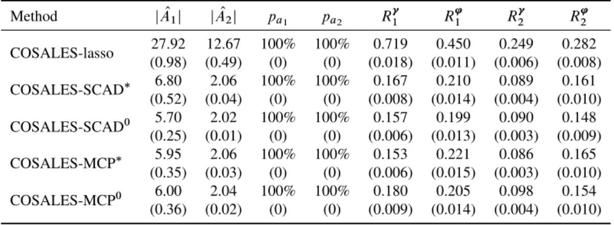
The results are summarized in Table 2.2, from which we can draw the following conclu-sions:

(1) The COSALES regression (with lasso or nonconvex penalties) can recover the sparse patterns in both the mean and scale functions with overwhelming probabilities. (2) The COSALES lasso tends to select a lot more irrelevant covariates and has much

larger estimation errors than the nonconvex penalized COSALES regression (with the SCAD penalty or MCP).

(3) The three-step LLA algorithm starting from zero produces similar results to the two-step LLA algorithm starting from the lasso solution.

EXAMPLE3. In this example, we simulate data from the following normal linear heteroscedastic model

y Dx6Cx12Cx15Cx20C.0:7x1C0:7x12/"; (2.17)

where the covariates are simulated by setting x1 D ˆ.z1/; x12 D ˆ.z12/; and xj D

zj; j ¤ 1; 12;where.z1; : : : ; zp/T

N.0;†/with † D .0:5ji jj/pp;and ˆ./ is the

CDF of the standard normal distribution. The random error " N.0; 1/: Note that in model (2.11), the active sets of the true parameter vectors do not overlap, so the SALES

(46)

Table 2.2: Numerical summary of simulation results from the lasso, SCAD and MCP penalized COSALES regression for model (2.11): y Dx6Cx12Cx15Cx20C.0:7x1/". The selection accuracy is measured by the number of selected variablesj OA1jandj OA2j, and the proportionspa1 and pa2 of covering the true active sets. The estimation accuracy is measured by theL1 risksR

1andR

'

1;and theL2risksR

2 andR

'

2:The results are shown as

averages over 100 replicates with standard errors listed in the parentheses. A fairly extreme

-value ( D0:95) is used in the simulation for easy separation of the mean and scale

Method j OA1j j OA2j pa1 pa2 R1 R ' 1 R 2 R ' 2 COSALES-lasso 26.88 13.36 100% 100% 0.407 0.378 0.124 0.294 (1.04) (0.45) (0) (0) (0.012) (0.008) (0.002) (0.006) COSALES-SCAD 7.24 1.01 100% 100% 0.095 0.072 0.048 0.072 (0.10) (0.01) (0) (0) (0.004) (0.005) (0.002) (0.005) COSALES-SCAD0 8.85 1.01 100% 100% 0.107 0.065 0.049 0.065 (0.57) (0.01) (0) (0) (0.005) (0.005) (0.002) (0.005) COSALES-MCP 6.46 1.01 100% 100% 0.089 0.070 0.045 0.070 (0.38) (0.01) (0) (0) (0.004) (0.005) (0.002) (0.005) COSALES-MCP0 7.08 1.01 100% 100% 0.102 0.067 0.052 0.067 (0.44) (0.01) (0) (0) (0.006) (0.005) (0.003) (0.005)

regression can detect active variables in the scale. However, in model (2.17) the active set for the mean, A1 D f6; 12; 15; 20g;overlaps with the active set for the scale, A2 D f1; 12g:Thus, the SALES regression cannot recover the variablex12in the scale function. We show by this Monte Carlo simulation that the COSALES regression can recover the sparse patterns in both the mean and scale functions. We fixp D600and independently simulate a training set of size n D 500 for fitting and a validation set of the same size for tuning. We select the regularization parameter by minimizing the validation error

P i2validation ˚ ‰0:5.yi xT ib/C‰.yi x T ib x T

ib'/ for the computed estimatebandb':In

order to separate the mean and scale easily, we again pick D 0:95. We implement the COSALES lasso and two variations of the LLA algorithm as were done in Examples 2 for each of the SCAD and MCP penalized COSALES regressions.

Based on 100 independent runs, the same measurements of performance as in Example 2 are calculated to evaluate the sparsity recovery and estimation accuracy of the COSALES

(47)

2.5. REALDATA EXAMPLE 31

estimation. The results are summarized in Table 2.3. Same conclusions in Example 2 can be drawn here.

Table 2.3: Numerical summary of simulation results from the the lasso, SCAD and MCP

penalized COSALES regression for model (2.17): y Dx6Cx12Cx15Cx20C.0:7x1C

0:7x12/". The selection accuracy is measured by the number of selected variables j OA1j

andj OA2j, and the proportionspa1 andpa2 of covering the true active sets. The estimation

accuracy is measured by theL1risksR

1 andR

'

1;and theL2 risksR

2 andR

'

2:The results

are shown as averages over 100 replicates with standard errors listed in the parentheses. A fairly extreme-value ( D0:95) is used in the simulation for easy separation of the mean and scale Method j OA1j j OA2j pa1 pa2 R1 R ' 1 R 2 R ' 2 COSALES-lasso 27.92 12.67 100% 100% 0.719 0.450 0.249 0.282 (0.98) (0.49) (0) (0) (0.018) (0.011) (0.006) (0.008) COSALES-SCAD 6.80 2.06 100% 100% 0.167 0.210 0.089 0.161 (0.52) (0.04) (0) (0) (0.008) (0.014) (0.004) (0.010) COSALES-SCAD0 5.70 2.02 100% 100% 0.157 0.199 0.090 0.148 (0.25) (0.01) (0) (0) (0.006) (0.013) (0.003) (0.009) COSALES-MCP 5.95 2.06 100% 100% 0.153 0.221 0.086 0.165 (0.35) (0.03) (0) (0) (0.006) (0.015) (0.003) (0.010) COSALES-MCP0 6.00 2.04 100% 100% 0.180 0.205 0.098 0.154 (0.36) (0.02) (0) (0) (0.009) (0.014) (0.004) (0.010)

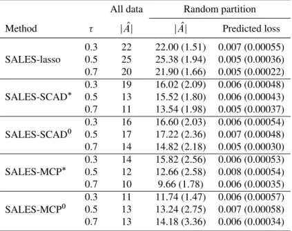
2.5 Real Data Example

We apply the SALES and COSALES regressions to a real data set reported inScheetz et al.

(2006). The data set consists of gene expression levels of more than 31,000 probes obtained from 120 rats. The expressions are analyzed on a logarithmic scale (base2). As was done inScheetz et al.(2006), we exclude the probes that were not expressed in the eye or that lacked sufficient variation. Among those 18,976 probes left, we study how the expressions of other genes are associated with the gene TRIM32(probe 1389163 at). This gene was found to be associated with Bardet–Biedl syndrome, which is a disorder that affects many parts of the body including the retina. For all the other genes, we first standardize them