Label ranking by learning pairwise preferences

Contents lists available atScienceDirect

Artificial Intelligence

www.elsevier.com/locate/artint

Label ranking by learning pairwise preferences

Eyke Hüllermeier

a,∗

, Johannes Fürnkranz

b

, Weiwei Cheng

a

, Klaus Brinker

a a_{Department of Mathematics and Computer Science, Philipps-Universität Marburg, Germany}

b_{Department of Computer Science, TU Darmstadt, Germany}

a r t i c l e i n f o a b s t r a c t

Article history:

Received 21 January 2008

Received in revised form 14 July 2008 Accepted 8 August 2008

Available online 15 August 2008 Keywords:

Preference learning Ranking

Pairwise classification Constraint classification

Preference learning is an emerging topic that appears in different guises in the recent literature. This work focuses on a particular learning scenario called label ranking, where the problem is to learn a mapping from instances to rankings over a finite number of labels. Our approach for learning such a mapping, called ranking by pairwise comparison (RPC), first induces a binary preference relation from suitable training data using a natural extension of pairwise classification. A ranking is then derived from the preference relation thus obtained by means of a ranking procedure, whereby different ranking methods can be used for minimizing different loss functions. In particular, we show that a simple (weighted) voting strategy minimizes risk with respect to the well-known Spearman rank correlation. We compare RPC to existing label ranking methods, which are based on scoring individual labels instead of comparing pairs of labels. Both empirically and theoretically, it is shown that RPC is superior in terms of computational efficiency, and at least competitive in terms of accuracy.

©2008 Elsevier B.V. All rights reserved.

1. Introduction

The topic of preferences has recently attracted considerable attention in Artificial Intelligence (AI) research, notably in

fields such as agents, non-monotonic reasoning, constraint satisfaction, planning, and qualitative decision theory [19].1

Pref-erences provide a means for specifying desires in a declarative way, which is a point of critical importance for AI. In fact, consider AI’s paradigm of a rationally acting (decision-theoretic) agent: The behavior of such an agent has to be driven by an underlying preference model, and an agent recommending decisions or acting on behalf of a user should clearly reflect that user’s preferences.

It is hence hardly surprising that methods for learning and predicting preferences in an automatic way are among the very recent research topics in disciplines such as machine learning, knowledge discovery, and recommender systems. Many approaches have been subsumed under the terms of ranking and preference learning, even though some of them are quite different and are not sufficiently well discriminated by existing terminology. We will thus start our paper with a clarification of its contribution (Section 2). The learning scenario that we will consider in this paper assumes a collection of training examples which are associated with a finite set of decision alternatives. Following the common notation of

supervised learning, we shall refer to the latter aslabels. However, contrary to standard classification, a training example is

not assigned a single label, but a set ofpairwise preferencesbetween labels (which neither has to be complete nor entirely

*

Corresponding author.

E-mail addresses:[email protected](E. Hüllermeier),juffi@ke.informatik.tu-darmstadt.de(J. Fürnkranz),[email protected] (W. Cheng),[email protected](K. Brinker).

1 _{The increasing activity in this area is also witnessed by several workshops that have been devoted to preference learning and related topics, such as} those at the NIPS-02, KI-03, SIGIR-03, NIPS-04, GfKl-05, IJCAI-05 and ECAI-2006 conferences (the second and fifth organized by two of the authors). 0004-3702/$ – see front matter ©2008 Elsevier B.V. All rights reserved.

Table 1

Four different approaches to learning from preference information together with representative references

modeling utility functions modeling pairwise preferences object ranking comparison training [58] learning to order things [13] label ranking constraint classification [28] this work[24]

consistent), each one expressing that one label is preferred over another. The goal is to learn to predict a total order, a

ranking, of all possible labels for a new training example.

Theranking by pairwise comparison(RPC) algorithm, which we introduce in Section 3 of this paper, has a modular struc-ture and works in two phases. First, pairwise preferences are learned from suitable training data, using a natural extension

of so-calledpairwise classification. Then, a ranking is derived from a set of such preferences by means of aranking procedure.

In Section 4, we analyze the computational complexity of the RPC algorithm. Then, in Section 5, it will be shown that, by using suitable ranking procedures, RPC can minimize the risk for certain loss functions on rankings. Section 6 is devoted to an experimental evaluation of RPC and a comparison with alternative approaches applicable to the same learning problem. The paper closes with a discussion of related work in Section 7 and concluding remarks in Section 8. Parts of this paper are based on [24,25,33].

2. Learning from preferences

In this section, we will motivate preference learning2 _{as a theoretically interesting and practically relevant subfield of}

machine learning. One can distinguish two types of preference learning problems, namely learning from object preferences

andlearning from label preferences, as well as two different approaches for modeling the preferences, namely byevaluating

individual alternatives (by means of a utility function), or by comparing (pairs of) competing alternatives (by means of a

preference relation). Table 1 shows the four possible combinations thus obtained. In this section, we shall discuss these options and show that our approach, label ranking by pairwise comparison, is still missing in the literature and hence a novel contribution.

2.1. Learning from object preferences

The most frequently studied problem in learning from preferences is to induce aranking function r

(

·

)

that is able to order

any subset

O

of an underlying class

X

of objects. That is,r

(

·

)

assumes as input a subset

O

= {

x1

. . .

xn

} ⊆

X

of objects and

returns as output a permutation

τ

of

{

1

. . .

n

}

. The interpretation of this permutation is that object xi is preferred to xj

whenever

τ

(

i

) <

τ

(

j

)

. The objects themselves (e.g. websites) are typically characterized by a finite set of features as in

conventional attribute-value learning. The training data consists of a set of exemplary pairwise preferences. This scenario, summarized in Fig. 1, is also known as “learning to order things” [13].

As an example consider the problem of learning to rank query results of a search engine [35,52]. The training information is provided implicitly by the user who clicks on some of the links in the query result and not on others. This information can be turned into binary preferences by assuming that the selected pages are preferred over nearby pages that are not clicked on [36].

2.2. Learning from label preferences

In this learning scenario, the problem is to predict, for any instance x (e.g., a person) from an instance space

X

, a

preference relation

x

⊆

L

×

L

among a finite set

L

= {

λ1

. . . λ

m

}

of labels or alternatives, where

λ

i

x

λ

j means that

instancexprefers the label

λ

ito the label

λ

j. More specifically, we are especially interested in the case where

x is a total

strict order, that is, a ranking of

L

. Note that a ranking

x can be identified with a permutation

τ

x of

{

1

. . .

m

}

, e.g., the

permutation

τ

x such that

τ

x

(

i

) <

τ

x

(

j

)

whenever

λ

i

x

λ

j (

τ

(

i

)

is the position of

λ

i in the ranking). We shall denote the

class of all permutations of

{

1

. . .

m

}

by

S

m. Moreover, by abuse of notation, we shall sometimes employ the terms “ranking”

and “permutation” synonymously.

The training information consists of a set of instances for which (partial) knowledge about the associated preference

relation is available (cf. Fig. 2). More precisely, each training instancexis associated with a subset of all pairwise preferences.

Thus, even though we assume the existence of an underlying (“true”) ranking, we do not expect the training data to provide full information about that ranking. Besides, in order to increase the practical usefulness of the approach, we even allow for inconsistencies, such as pairwise preferences which are conflicting due to observation errors.

2 _{We interpret the term “preference” not literally but in a wide sense as a kind of order relation. Thus,abcan indeed mean that alternativeais more} liked by a person thanb, but also thatais an algorithm that outperformsbon a certain problem, thatais an event that is more probable thanb, thata is a student finishing her studies beforeb, etc.

Given:

•a (potentially infinite) reference set of objectsX

(each object typically represented by a feature vector) •a finite set of pairwise preferencesxixj,(xi,xj)∈X×X

Find:

•a ranking functionr(·)that assumes as input a set of objectsO⊆Xand returns a permutation (ranking) of this set

Fig. 1.Learning from object preferences.

Given:

•a set of training instances{xk|k=1. . .n} ⊆X (each instance typically represented by a feature vector) •a set of labelsL= {λi|i=1. . .m}

•for each training instancexk: a set ofpairwise preferencesof the form

λixkλj Find:

•a ranking function that maps anyx∈Xto a rankingxofL(permutation

τx∈Sm)

Fig. 2.Learning from label preferences.

As in the case of object ranking, this learning scenario has a large number of practical applications. In the empirical part, we investigate the task of predicting a “qualitative” representation of a gene expression profile as measured by microarray analysis from phylogenetic profile features [4]. Another application scenario is meta-learning, where the task is to rank learning algorithms according to their suitability for a new dataset, based on the characteristics of this dataset [10]. Finally, every preference statement in the well-known CP-nets approach [7], a qualitative graphical representation that reflects

conditional dependence and independence of preferences under aceteris paribus interpretation, formally corresponds to a

label ranking.

In addition, it has been observed by several authors [17,24,28] that many conventional learning problems, such as classi-fication and multi-label classiclassi-fication, may be formulated in terms of label preferences:

•

Classification:A single class label

λ

iis assigned to each examplexk. This implicitly defines the set of preferences

{

λ

i

xk

λ

j

|

1

j

=

i

m

}

.

•

Multi-label classification:Each training examplexk is associated with a subset Lk

⊆

L

of possible labels. This implicitly defines the set of preferences

{

λ

i

xk

λ

j

|

λ

i

∈

Lk

, λ

j

∈

L

\

Lk

}

.

In each of the former scenarios, a ranking model f:

X

→

S

m is learned from a subset of all possible pairwise preferences.

A suitable projection may be applied to the ranking model (which outputs permutations) as a post-processing step, for example a projection to the top-rank in classification learning where only this label is relevant.

2.3. Learning utility functions

As mentioned above, one natural way to represent preferences is to evaluate individual alternatives by means of a

(real-valued) utility function. In the object preferences scenario, such a function is a mapping f:

X

→

R

that assigns a utility

degree f

(

x

)

to each objectxand, hence, induces a complete order on

X

. In the label preferences scenario, a utility function

fi:

X

→

R

is needed for each of the labels

λ

i,i

=

1

. . .

m. Here, fi

(

x

)

is the utility assigned to alternative

λ

iby instance x. To obtain a ranking forx, the alternatives are ordered according to these utility scores, i.e.,

λ

i

x

λ

j

⇔

fi

(

x

)

fj

(

x

)

.

If the training data would offer the utility scores directly, preference learning would reduce to a standard regression problem (up to a monotonic transformation of the utility values). This information can rarely be assumed, however. Instead, usually only constraints derived from comparative preference information of the form “This object (or label) should have a higher utility score than that object (or label)” are given. Thus, the challenge for the learner is to find a function that is as much as possible in agreement with all constraints.

For object ranking approaches, this idea has first been formalized by Tesauro [58] under the namecomparison training.

He proposed a symmetric neural-network architecture that can be trained with representations of two states and a training signal that indicates which of the two states is preferable. The elegance of this approach comes from the property that one can replace the two symmetric components of the network with a single network, which can subsequently provide a real-valued evaluation of single states. Later works on learning utility function from object preference data include [27,31, 35,60]

Subsequently, we outline two approaches, constraint classification (CC) and log-linear models for label ranking (LL), that are direct alternatives to our method of ranking by pairwise comparison, and that we shall later on compare with.

2.3.1. Constraint classification

For the case of label ranking, a corresponding method for learning the functions fi

(

·

)

,i

=

1

. . .

m, from training data has

been proposed in the framework ofconstraint classification[28,29]. Proceeding from linear utility functions

fi

(

x

)

=

n

k=1

α

ikxk (2.1)

with label-specific coefficients

α

ik,k

=

1

. . .

n, a preference

λ

i

x

λ

jtranslates into the constraint fi

(

x

)

−

fj

(

x

) >

0 or,

equiva-lently, fj

(

x

)

−

fi

(

x

) <

0. Both constraints, the positive and the negative one, can be expressed in terms of the sign of an inner

product

z

,

α

, where

α

=

(

α

11

. . .

α

1n

,

α

21

. . .

α

mn

)

is a concatenation of all label-specific coefficients. Correspondingly, the

vector z is constructed by mapping the original

-dimensional training examplex

=

(

x1

. . .

x

)

into an

(

m

×

)

-dimensional

space: For the positive constraint, x is copied into the components

((

i

−

1

)

×

+

1

) . . . (

i

×

)

and its negation

−

x into

the components

((

j

−

1

)

×

+

1

) . . . (

j

×

)

; the remaining entries are filled with 0. For the negative constraint, a vector

is constructed with the same elements but reversed signs. Both constraints can be considered as training examples for a

conventional binary classifier in an

(

m

×

)

-dimensional space: The first vector is a positive and the second one a negative

example. The corresponding learner tries to find a separating hyperplane in this space, that is, a suitable vector

α

satisfying

all constraints. For classifying a new examplee, the labels are ordered according to the response resulting from

multiply-ing e with thei-th

-element section of the hyperplane vector. To work with more general types of utility functions, the

method can obviously be kernelized.

Alternatively, Har-Peled et al. [28,29] propose an online version of constraint classification, namely an iterative algorithm

that maintains weight vectors

α

1

. . .

α

m

∈

R

for each label individually. In every iteration, the algorithm checks each

con-straint

λ

i

x

λ

jand, in case the associated inequality

α

i

×

x

=

fi

(

x

) >

fj

(

x

)

=

α

j

×

xis violated, adapts the weight vectors

α

i

,

α

j appropriately. In particular, using perceptron training, the algorithm can be implemented in terms of a multi-output

perceptron in a way quite similar to the approach of Grammer and Singer [15].

2.3.2. Log-linear models for label ranking

So-called log-linear models for label ranking have been proposed in Dekel et al. [17]. Here, utility functions are expressed

in terms of linear combinations of a set ofbase ranking functions:

fi

(

x

)

=

j

α

jhj

(

x

, λ

i

),

where a base functionhj

(

·

)

maps instance/label pairs to real numbers. Interestingly, for the special case in which instances

are represented as feature vectors x

=

(

x1

. . .

x

)

and the base functions are of the form

hkj

(

x

, λ)

=

xk

λ

=

λ

j

0

λ

=

λ

j

(

1

k

,

1

j

m

),

(2.2)

the approach is essentially equivalent to CC, as it amounts to learning class-specific utility functions (2.1). Algorithmically, however, the underlying optimization problem is approached in a different way, namely by means of a boosting-based algorithm that seeks to minimize a (generalized) ranking error in an iterative way.

2.4. Learning preference relations

The key idea of this approach is to model the individual preferences directly instead of translating them into a utility function. This seems a natural approach, since it has already been noted that utility scores are difficult to elicit and observed preferences are usually of the relational type. For example, it is very hard to ensure a consistent scale even if all utility evaluations are performed by the same user. The situation becomes even more problematic if utility scores are elicited from different users, which may not have a uniform scale of their scores [13]. For the learning of preferences, one may bring up a similar argument. It will typically be easier to learn a separate theory for each individual preference that compares two objects or two labels and determines which one is better. Of course, every learned utility function that assigns a score to a

set of labels

L

induces such a binary preference relation on these labels.

For object ranking problems, the pairwise approach has been pursued in [13]. The authors propose to solve object ranking

problems by learning a binary preference predicate Q

(

x

,

x

)

, which predicts whetherxis preferred toxor vice versa. A final

ordering is found in a second phase by deriving a ranking that is maximally consistent with these predictions.

For label ranking problems, the pairwise approach has been introduced by Fürnkranz and Hüllermeier [24]. The key

idea, to be described in more detail in Section 3, is to learn, for each pair of labels

(λ

i

, λ

j

)

, a binary predicate

M

i j

(

x

)

that

predicts whether

λ

i

x

λ

jor

λ

j

x

λ

ifor an inputx. In order to rank the labels for a new object, predictions for all pairwise

label preferences are obtained and a ranking that is maximally consistent with these preferences is derived.

3. Label ranking by learning pairwise preferences

The key idea ofranking by pairwise comparison(RPC) is to reduce the problem of label ranking to several binary

a ranking using a separate ranking algorithm (Section 3.3). We consider thismodularityof RPC as an important advantage of the approach. Firstly, the binary classification problems are comparably simple and efficiently learnable. Secondly, as will become clear in the remainder of the paper, different ranking algorithms allow the ensemble of pairwise classifiers to adapt to different loss functions on label rankings without the need for re-training the pairwise classifiers.

3.1. Pairwise classification

The key idea of pairwise learning is well-known in the context of classification [22], where it allows one to transform a

multi-class classification problem, i.e., a problem involvingm

>

2 classes

L

= {

λ1

. . . λ

m

}

, into a number ofbinaryproblems.

To this end, a separate model (base learner)

M

i j is trained for eachpairof labels

(λ

i

, λ

j

)

∈

L

, 1

i

<

j

m; thus, a total

number ofm

(

m

−

1

)/

2 models is needed.

M

i j is intended to separate the objects with label

λ

ifrom those having label

λ

j.

At classification time, a query instance is submitted to all models

M

i j, and their predictions are combined into an overall

prediction. In the simplest case, each prediction of a model

M

i j is interpreted as a vote for either

λ

i or

λ

j, and the label

with the highest number of votes is proposed as a final prediction.3

Pairwise classification has been tried in the areas of statistics [8,21], neural networks [40,41,44,51], support vector ma-chines [30,32,42,54], and others. Typically, the technique learns more accurate theories than the more commonly used one-against-all classification method, which learns one theory for each class, using the examples of this class as positive

examples and all others as negative examples.4 Surprisingly, it can be shown that pairwise classification is also

computa-tionally more efficient than one-against-all class binarization (cf. Section 4).

3.2. Learning pairwise preference

The above procedure can be extended to the case of preference learning in a natural way [24]. Again, a preference

(order) information of the form

λ

a

x

λ

b is turned into a training example

(

x

,

y

)

for the learner

M

i j, wherei

=

min

(

a

,

b

)

and j

=

max

(

a

,

b

)

. Moreover,y

=

1 ifa

<

band y

=

0 otherwise. Thus,

M

i j is intended to learn the mapping that outputs

1 if

λ

i

x

λ

j and 0 if

λ

j

x

λ

i:

x

→

1 if

λ

i

x

λ

j

,

0 if

λ

j

x

λ

i

.

(3.1)

The model is trained with all examples xk for which either

λ

i

xk

λ

j or

λ

j

xk

λ

i is known. Examples for which nothing is

known about the preference between

λ

iand

λ

jare ignored.

The mapping (3.1) can be realized by any binary classifier. Alternatively, one may also employ base classifiers that map

into the unit interval

[

0

,

1

]

instead of

{

0

,

1

}

, and thereby assign a valued preference relation

R

x to every (query) instance

x

∈

X

:

R

x

(λ

i

, λ

j

)

=

M

i j

(

x

)

ifi

<

j

,

1

−

M

ji

(

x

)

ifi

>

j (3.2)

for all

λ

i

=

λ

j

∈

L

. The output of a

[

0

,

1

]

-valued classifier can usually be interpreted as a probability or, more generally, a

kind of confidence in the classification: the closer the output of

M

i j to 1, the stronger the preference

λ

i

x

λ

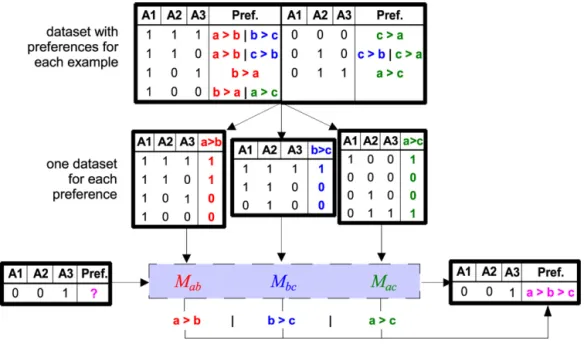
jis supported.

Fig. 3 illustrates the entire process for a hypothetical dataset with eight examples that are described with three binary

attributes (A1, A2, A3) and preferences among three labels (a, b, c). First, the original training set is transformed into three

two-class training sets, one for each possible pair of labels, containing only those training examples for which the relation

between these two labels is known. Then three binary models,

M

ab,

M

bc, and

M

ac are trained. In our example, the result

could be simple rules like the following:

M

ab: a

>

b if A2

=

1

.

M

bc: b

>

c if A3

=

1

.

M

ac: a

>

c if A1

=

1

∨

A3

=

1

.

Given a new example with an unknown preference structure (shown in the bottom left of Fig. 3), the predictions of these models are then used to predict a ranking for this example. As we will see in the next section, this is not always as trivial as in this example.

3 _{Ties can be broken in favor or prevalent classes, i.e., according to the class distribution in the classification setting.}

4 _{Rifkin and Klautau [53] have argued that, at least in the case of support vector machines, one-against-all can be as effective provided that the binary} base classifiers are carefully tuned.

Fig. 3.Schematic illustration of learning by pairwise comparison.

3.3. Combining predicted preferences into a ranking

Given a predicted preference relation

R

x for an instance x, the next question is how to derive an associated ranking

τ

x.

This question is non-trivial, since a relation

R

x does not always suggest a unique ranking in an unequivocal way. For

exam-ple, the learned preference relation need not be transitive (cf. Section 3.4). In fact, the problem of inducing a ranking from a (valued) preference relation has received a lot of attention in several research fields, e.g., in fuzzy preference modeling and (multi-attribute) decision making [20]. In the context of pairwise classification and preference learning, several studies have empirically compared different ways of combining the predictions of individual classifiers [2,23,34,62].

A simple though effective strategy is a generalization of the aforementioned voting strategy: each alternative

λ

i is

eval-uated by the sum of (weighted) votes

S

(λ

i

)

=

λj=λi

R

x

(λ

i

, λ

j

),

(3.3)

and all labels are then ordered according to these evaluations, i.e., such that

(λ

i

x

λ

j

)

⇒

S

(λ

i

)

S

(λ

j

)

.

(3.4)

Even though this ranking procedure may appear rather ad-hoc at first sight, we shall give a theoretical justification in Section 5, where it will be shown that ordering the labels according to (3.3) minimizes a reasonable loss function on rankings.

3.4. Transitivity

Our pairwise learning scheme as outlined above produces a relation

R

x by learning the preference degrees

R

x

(λ

i

, λ

j

)

independently of each other. In this regard, one may wonder whether there are no interdependencies between these

de-grees that should be taken into account. In particular, as transitivityof pairwise preferences is one of the most important

properties in preference modeling, an interesting question is whether any sort of transitivity can be guaranteed for

R

x.

Obviously, the learned binary preference relation does not necessarily have the typical properties of order relations. For

example, transitivity will in general not hold, because if

λ

i

x

λ

jand

λ

j

x

λ

k, the independently trained classifier

M

ikmay

still predict

λ

k

x

λ

i.5 This is not a problem, because the subsequent ranking phase will convert the intransitive predictive

preference relation into a total preference order.

However, it can be shown that, given the formal assumptions of our setting, the following weak form of transitivity must be satisfied:

∀

i

,

j

,

k

∈ {

1

. . .

m

}

:

R

x

(λ

i

, λ

j

)

R

x

(λ

i

, λ

k

)

+

R

x

(λ

k

, λ

j

)

−

1

.

(3.5) 5 _{In fact, not even symmetry needs to hold ifM}

i jandMjiare different models, which is, e.g., the case for rule learning algorithms [22]. This situation may be compared with round robin sports tournament, where individual results do not necessarily conform to the final ranking that is computed from them.

As a consequence of this property, which is proved in Appendix A, the predictions obtained by an ensemble of pairwise

learners

M

i j should actually satisfy (3.5). In other words, training the learners independently of each other is indeed not

fully legitimate. Fortunately, our experience so far has shown that the probability to violate (3.5) is not very high. Still, forcing (3.5) to hold is a potential point of improvement and part of ongoing work.

4. Complexity analysis

In this section, we will generalize previous results on the efficiency of pairwise classification to preference learning. In particular, we will show that this approach can be expected to be computationally more efficient than alternative approaches like constraint classification that try to model the preference learning problem as a single binary classification problem in a higher-dimensional space (cf. Section 2.3).

4.1. Ranking by pairwise comparison

First, we will bound the number of training examples used by the pairwise approach. Let

|

Pk

|

be the number of

prefer-ences that are associated with example xk. Throughout this section, we denote byd

=

1

/

n

·

k

|

Pk

|

the average number of

preferences over all examples.

Lemma 1.The total number of training examples constructed by RPC is n

·

d, which is bounded by n

·

m

(

m

−

1

)/

2, i.e.,

n

k=1

|

Pk

| =

n

·

d

n

·

m

(

m

−

1

)

2

.

Proof. Each of thentraining examples will be added to all

|

Pk

|

binary training sets that correspond to one of its preferences.

Thus, the total number of training examples is

n_k=1

|

Pk

| =

n

·

d. This is bounded from above by the size of a complete set

of preferencesn

·

m

(

m

−

1

)/

2.

2

The special case for classification, where the number of training examples grow only linearly with the number of classes

[22], can be obtained as a corollary of this theorem, because for classification, each class label expands to d

=

m

−

1

preferences.

As a consequence, it follows immediately that RPC using a base algorithm with a linear run-time complexity

O

(

n

)

has a

total run-time of

O

(

d

·

n

)

. More interesting is the general case.

Theorem 1.For a base learner with complexity

O

(

na

)

, the complexity of RPC is

O

(

d

·

na

)

.

Proof. Letni j be the number of training examples for model

M

i j. Each example corresponds to a single preference, i.e.,

1i<jm ni j

=

n

k=1

|

Pk

| =

d

·

n

and the total learning complexity is

O

(

na

i j

)

. We now obtain

O

(

na_{i j}

)

O

(

d

·

na

₎

=

1 d

O

(

na_{i j}

)

O

(

na

₎

=

1 d

O

ni j n

a

1 d

O

ni j n

=

O

(

ni j

)

d

·

O

(

n

)

=

O

(

ni j

)

O

(

d

·

n

)

=

O

(

d

·

n

)

O

(

d

·

n

)

=

O

(

1

).

The inequality holds because each example can have at most one preference involving the pair of labels

(λ

i

, λ

j

)

. Thus,

ni j

n.

2

Again, we obtain as a corollary that the complexity of pairwise classification is only linear in the number of classes

O

(

m

·

na

₎

_{, for which an incomplete proof was previously given in [22].}

4.2. Constraint classification and log-linear models

For comparison, CC converts each example into a set of examples, one positive and one negative for each preference. This construction leads to the following complexity.

Proof. CC transforms the original training data into a set of 2

n_k=1

|

Pk

| =

2dn examples, which means that CC constructs

twice as many training examples as RPC. If this problem is solved with a base learner with complexity

O

(

na

₎

_{, the total}

complexity is

O

((

2dn

)

a

)

=

O

(

da

_·

_na

₎

_.

₂

Moreover, the newly constructed examples are projected into a space that hasmtimes as many attributes as the original

space.

A direct comparison is less obvious for the online version of CC whose complexity strongly depends on the number of iterations needed to achieve convergence. In a single iteration, the algorithm checks all constraints for every instance and,

in case a constraint is violated, adapts the weight vector correspondingly. The complexity is hence

O

(

n

·

d

·

·

T

)

, where

is

the number of attributes of an instance (dimension of the instance space) and T the number of iterations.

For the same reason, it is difficult to compare RPC with the boosting-based algorithm proposed for log-linear models by Dekel et al. [17]. In each iteration, the algorithm essentially updates the weights that are associated with each instance

and preference constraint. In the label ranking setting considered here, the complexity of this step is

O

(

d

·

n

)

. Moreover,

the algorithm maintains weight coefficients for each base ranking function. If specified as in (2.2), the number of these

functions ism

·

. Therefore, the total complexity of LL is

O

((

d

·

n

+

m

·

)

·

T

)

, withT the number of iterations.

4.3. Discussion

In summary, the overall complexity of pairwise label ranking depends on the average number of preferences that are given for each training example. While being quadratic in the number of labels if a complete ranking is given, it is only linear for the classification setting. In any case, it is no more expensive than constraint classification and can be considerably

cheaper if the complexity of the base learner is super-linear (i.e.,a

>

1). The comparison between RPC and LL is less obvious

and essentially depends on how na _{relates ton}

_·

_{T (note that, implicitly, T also depends onn, as larger data sets typically}

need more iterations).

A possible disadvantage of RPC concerns the large number of classifiers that have to be stored. Assuming an input space

X

of dimensionality

and simple linear classifiers as base learners, the pairwise approach has to store

O

(

·

m2

)

parameters,

whereas both CC and LL only need to store

O

(

·

m

)

parameters to represent their ranking model. (During training, however,

the boosting-based optimization algorithm in LL must also store a typically much higher number ofn

·

dparameters, one

for each preference constraint.)

As all the model parameters have to be used for deriving a label ranking, this may also affect the prediction time. However, for the classification setting, it was shown in [48] that a more efficient algorithm yields the same predictions as

voting in almost linear time (

≈

O

(

·

m

)

). To what extent this algorithm can be generalized to label ranking is currently

under investigation. As ranking is basically a sorting of all possible labels, we expect that this can be done in log-linear time (

O

(

·

mlogm

)

).

5. Risk minimization

Even though the approach to pairwise ranking as outlined in Section 3 appears intuitively appealing, one might argue that it lacks a solid foundation and remains ad-hoc to some extent. For example, one might easily think of ranking proce-dures other than (3.3), leading to different predictions. In any case, one might wonder whether the rankings predicted on the basis of (3.2) and (3.3) do have any kind of optimality property. An affirmative answer to this question will be given in this section.

5.1. Preliminaries

Recall that, in the setting of label ranking, we associate every instance xfrom an instance space

X

with a ranking of

a finite set of class labels

L

= {

λ1

. . . λ

m

}

or, equivalently, with a permutation

τ

x

∈

S

m (where

S

m denotes the class of all

permutations of

{

1

. . .

m

}

). More specifically, and in analogy with the setting of conventional classification, every instance is

associated with a probability distribution over the class of rankings (permutations)

S

m. That is, for every instance x, there

exists a probability distribution

P

(

· |

x

)

such that, for every

τ

∈

S

m,

P

(

τ

|

x

)

is the probability to observe the ranking

τ

as

an output, given the instancexas an input.

The quality of a model

M

(induced by a learning algorithm) is commonly measured in terms of itsexpected lossorrisk

E

D

y

,

M

(

x

)

,

(5.1)

where D

(

·

)

is a loss or distance function,

M

(

x

)

denotes the prediction made by the model for the instancex, and yis the

true outcome. The expectation

E

is taken over

X

×

Y

, where

Y

is the output space;6_{in our case,}

_Y

_{is given by}

_S

m.

5.2. Spearman’s rank correlation

An important and frequently applied similarity measure for rankings is theSpearman rank correlation, originally proposed

by Spearman [57] as a nonparametric rank statistic to measure the strength of the associations between two variables [43]. It is defined as follows

1

−

6D

(

τ

,

τ

₎

m

(

m2

₋

₁

₎

(5.2)

as a linear transformation (normalization) of the sum of squared rank distances

D

(

τ

,

τ

)

=

df m

i=1

τ

(

i

)

−

τ

(

i

)

2 (5.3)

to the interval

[−

1

,

1

]

. As will now be shown, RPC is a risk minimizer with respect to (5.3) (and hence Spearman rank

correlation) as a distance measure under the condition that the binary models

M

i j provide correct probability estimates,

i.e.,

R

x

(λ

i

, λ

j

)

=

M

i j

(

x

)

=

P

(λ

i

x

λ

j

).

(5.4)

That is, if (5.4) holds, then RPC yields a risk minimizing prediction

ˆ

τ

x

=

arg min τ∈Sm

τ∈Sm D

(

τ

,

τ

)

·

P

(

τ

|

x

)

(5.5)

ifD

(

·

)

is given by (5.3). Admittedly, (5.4) is a relatively strong assumption, as it requires the pairwise preference

probabil-ities to be perfectly learnable. Yet, the result (5.5) sheds light on the aggregation properties of our technique under ideal

conditions and provides a valuable basis for further analysis. In fact, recalling that RPC consists of two steps, namely

pair-wise learningandranking, it is clear that in order to study properties of the latter, some assumptions about the result of the former step have to be made. And even though (5.4) might at best hold approximately in practice, it seems to be at least as natural as any other assumption about the output of the ensemble of pairwise learners.

Lemma 2.Let si, i

=

1

. . .

m, be real numbers such that0

s1

s2

· · ·

sm. Then, for all permutations

τ

∈

S

m, m

i=1

(

i

−

si

)

2

m

i=1

(

i

−

sτ(i)

)

2

.

(5.6) Proof. We have m

i=1

(

i

−

sτ(i)

)

2

=

m

i=1

(

i

−

si

+

si

−

sτ(i)

)

2

=

m

i=1

(

i

−

si

)

2

+

2 m

i=1

(

i

−

si

)(

si

−

sτ(i)

)

+

m

i=1

(

si

−

sτ(i)

)

2

.

Expanding the last equation and exploiting that

m_i=1s2

i

=

m i=1s2τ(i)yields m

i=1

(

i

−

sτ(i)

)

2

=

m

i=1

(

i

−

si

)

2

+

2 m

i=1 i si

−

2 m

i=1 i sτ(i)

.

On the right-hand side of the last equation, only the last term

m_i=1isτ(i)depends on

τ

. This term is maximal for

τ

(

i

)

=

i,

becausesi

sjfori

<

j, and therefore maxi=1...mmsi

=

msm, maxi=1...m−1(m

−

1

)

si

=

(

m

−

1

)

sm−1, etc. Thus, the difference

of the two sums is always positive, and the right-hand side is larger than or equal to

m_i=1

(

i

−

si

)

2, which proves the

lemma.

2

Lemma 3.Let

P

(

· |

x

)

be a probability distribution over

S

m. Moreover, let

si df

=

m

−

j=i

P

(λ

i

x

λ

j

)

(5.7) with

P

(λ

i

x

λ

j

)

=

τ:τ(i)<τ(j)

P

(

τ

|

x

).

(5.8) Then, si

=

_τ

P

(

τ

|

x

)

τ

(

i

)

.

Proof. We have si

=

m

−

j=i

P

(λ

i

x

λ

j

)

=

1

+

j=i

1

−

P

(λ

i

x

λ

j

)

=

1

+

j=i

P

(λ

j

x

λ

i

)

=

1

+

j=i

τ:τ(j)<τ(i)

P

(

τ

|

x

)

=

1

+

τ

P

(

τ

|

x

)

j=i

1 if

τ

(

i

) >

τ

(

j

)

0 if

τ

(

i

) <

τ

(

j

)

=

1

+

τ

P

(

τ

|

x

)

τ

(

i

)

−

1

=

τ

P

(

τ

|

x

)

τ

(

i

).

2

Note that si

sj is equivalent to S

(λ

i

)

S

(λ

j

)

(as defined in (3.3)) under the assumption (5.4). Thus, ranking the

alternatives according to S

(λ

i

)

(in decreasing order) is equivalent to ranking them according tosi(in increasing order).

Theorem 3.The expected distance

E

D

(

τ

,

τ

)

|

x

=

τ

P

(

τ

|

x

)

·

D

(

τ

,

τ

)

=

τ

P

(

τ

|

x

)

m

i=1

τ

(

i

)

−

τ

(

i

)

2

becomes minimal by choosing

τ

such that

τ

(

i

)

τ

(

j

)

whenever si

sj, with sigiven by(5.7).

Proof. We have

E

D

(

τ

,

τ

)

|

x

=

τ

P

(

τ

|

x

)

m

i=1

τ

(

i

)

−

τ

(

i

)

2

=

m

i=1

τ

P

(

τ

|

x

)

τ

(

i

)

−

τ

(

i

)

2

=

m

i=1

τ

P

(

τ

|

x

)

τ

(

i

)

−

si

+

si

−

τ

(

i

)

2

=

m

i=1

τ

P

(

τ

|

x

)

τ

(

i

)

−

si

2

−

2

τ

(

i

)

−

si

si

−

τ

(

i

)

+

si

−

τ

(

i

)

2

=

m

i=1

τ

P

(

τ

|

x

)

τ

(

i

)

−

si

2

−

2

si

−

τ

(

i

)

τ

P

(

τ

|

x

)

τ

(

i

)

−

si

+

τ

P

(

τ

|

x

)

si

−

τ

(

i

)

2

.

In the last equation, the mid-term on the right-hand side becomes 0 according to Lemma 3. Moreover, the last term

obviously simplifies to

(

si

−

τ

(

i

))

2, and the first term is a constantc

=

τ

P

(

τ

|

x

)(

τ

(

i

)

−

si

)

2 that does not depend on

τ

.

Thus, we obtain

E

(

D

(

τ

,

τ

)

|

x

)

=

c

+

m_i=1

(

si

−

τ

(

i

))

2and the theorem follows from Lemma 2.

2

5.3. Kendall’s tau

The above result shows that our approach to label ranking in the form presented in Section 3 is particularly tailored to (5.3) as a loss function. We like to point out, however, that RPC is not restricted to this measure but can also minimize other loss functions. As mentioned previously, this can be accomplished by replacing the ranking procedure in the second

step of RPC in a suitable way. To illustrate, consider the well-knownKendall tau measure[38] as an alternative loss function.

This measure essentially calculates the number of pairwise rank inversions on labels to measure the ordinal correlation of two rankings; more formally, with

denoting the number ofdiscordantpairs of items (labels), the Kendall tau coefficient is given by 1

−

4D

(

τ

,

τ

)/(

m

(

m

−

1

))

, that is, by a linear scaling of D

(

τ

,

τ

)

to the interval

[−

1

,

+

1

]

.

Now, for every ranking

τ

,

E

D

(

τ

,

τ

)

|

x

=

τ∈Sm

P

(

τ

)

×

D

(

τ

,

τ

)

=

τ∈Sm

P

(

τ

|

x

)

×

i<j|τ(i)<τ(j)

1 if

τ

(

i

) >

τ

(

j

)

0 if

τ

(

i

) <

τ

(

j

)

(5.10)

=

i<j|τ(i)<τ(j)

τ∈Sm

P

(

τ

|

x

)

×

1 if

τ

(

i

) >

τ

(

j

)

0 if

τ

(

i

) <

τ

(

j

)

=

i<j|τ(i)<τ(j)

P

(λ

i

x

λ

j

).

(5.11)

Thus, knowing the pairwise probabilities

P

(λ

i

x

λ

j

)

is again enough to derive the expected loss for every ranking

τ

. In

other words, RPC can also make predictions which are optimal for (5.9) as an underlying loss function. To this end, only the ranking procedure has to be adapted while the same pairwise probabilities (predictions of the pairwise learners) can be used.

Finding the ranking that minimizes (5.10) is formally equivalent to solving the graph-theoreticalfeedback arc setproblem

(for weightedtournaments) which is known to be NP complete [3]. Of course, in the context of label ranking, this result should be put into perspective, because the set of class labels is typically of small to moderate size. Nevertheless, from a computational point of view, the ranking procedure that minimizes Kendall’s tau is definitely more complex than the procedure for minimizing Spearman’s rank correlation.

5.4. Connections with voting theory

It is worth mentioning that the voting strategy in RPC, as discussed in Section 5.2, is closely related to the so-called

Borda-count, a voting rule that is well-known in social choice theory [9]: Suppose that the preferences of n voters are

expressed in terms of rankings

τ

1,

τ

2

. . .

τ

n of m alternatives. From a ranking

τ

i, the following scores are derived for the

alternatives: The best alternative receivesm

−

1 points, the second best m

−

2 points, and so on. The overall score of an

alternative is the sum of points that it has received from all voters, and a representative ranking

τ

ˆ

(aggregation of the single

voters’ rankings) is obtained by ordering the alternatives according to these scores.

Now, it is readily verified that the result obtained by this procedure corresponds exactly to the result of RPC if the

probability distribution over the class

S

m of rankings is defined by the corresponding relative frequencies. In other words,

the ranking

τ

ˆ

obtained by RPC minimizes the sum of all distances:

ˆ

τ

=

arg min τ∈Sm n

i=1 D

(

τ

,

τ

i

).

(5.12)

A ranking of that kind is sometimes calledcentral ranking.7

In connection with social choice theory it is also interesting to note that RPC does not satisfy the so-calledCondorcet

criterion: As the pairwise preferences in our above example show, it is thoroughly possible that an alternative (in this

case

λ1

) is preferred in all pairwisecomparisons (

R

(λ1, λ2) > .

5 and

R

(λ1, λ3) > .

5) without being the overall winner of

the election (top-label in the ranking). Of course, this apparently paradoxical property is not only relevant for ranking but also for classification. In this context, it has already been recognized by Hastie and Tibshirani [30].

Another distance (similarity) measure for rankings, which plays an important role in voting theory, is the

aforemen-tionedKendall tau. When using the number of discordant pairs (5.9) as a distance measure D

(

·

)

in (5.12),

τ

ˆ

is also called

the Kemeny-optimal ranking. Kendall’s tau is intuitively quite appealing and Kemeny-optimal rankings have several nice properties. However, as noted earlier, one drawback of using Kendall’s tau instead of rank correlation as a distance mea-sure in (5.12) is a loss of computational efficiency. In fact, the computation of Kemeny-optimal rankings is known to be NP-hard [5].

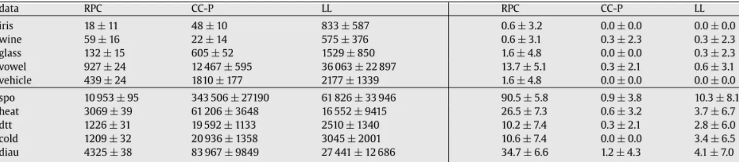
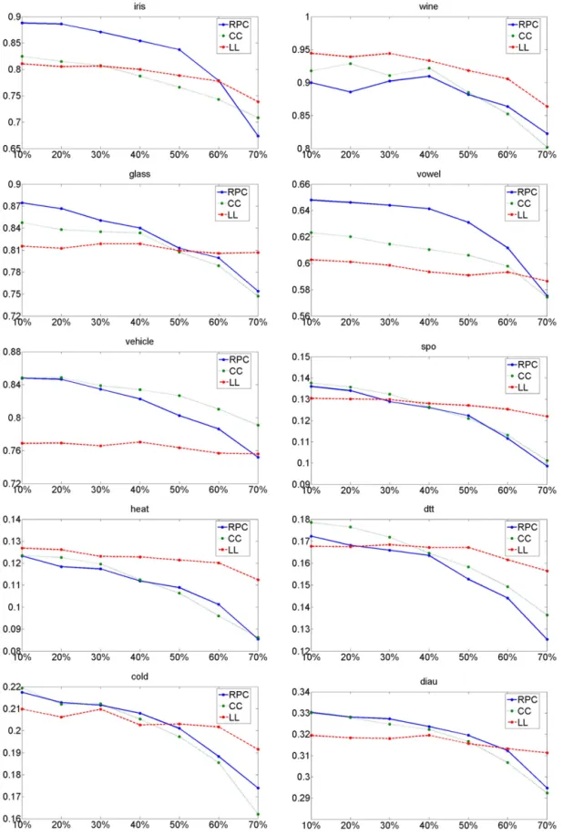
6. Empirical evaluation

The experimental evaluation presented in this section compares, in terms of accuracy and computational efficiency, ranking by pairwise comparison (RPC) with weighted voting to the constraint classification (CC) approach and log-linear models for label ranking (LL) as outlined, respectively, in Sections 2.3.1 and 2.3.2. CC in particular is a natural counterpart

Table 2

Statistics for the semi-synthetic and real datasets

dataset #examples #classes #features

iris 150 3 4 wine 178 3 13 glass 214 6 9 vowel 528 11 10 vehicle 846 4 18 spo 2465 11 24 heat 2465 6 24 dtt 2465 4 24 cold 2465 4 24 diau 2465 7 24

to compare with, as its approach is orthogonal to ours: instead of breaking up the label ranking problem into a set of small pairwise learning problems, as we do, CC embeds the original problem into a single learning problem in a high-dimensional

feature space. We implemented CC with support vector machines using a linear kernel as a binary classifier (CC-SVM).8

Apart from CC in its original version, we also included an online-variant (CC-P) as proposed in [28], using a noise-tolerant

perceptron algorithm as a base learner [37].9

To guarantee a fair comparison, we use LL with (2.2) as base ranking functions, which means that it is based on the

same underlying model class as CC. Moreover, we implement RPC with simple logistic regression as a base learner,10_which

comes down to fitting a linear model and using the logistic link function (logit

(

π

)

=

log

(

π

/(

1

−

π

))

) to derive

[

0

,

1

]

-valued

scores, the type of model output requested in RPC. Essentially, all three approaches are therefore based on linear models

and, in fact, they all produce linear decision boundaries between classes.11 _{Nevertheless, to guarantee full comparability}

between RPC and CC, we also implemented the latter with logistic regression as a base learner (CC-LR).

6.1. Datasets

To provide a comprehensive analysis under varying conditions, we considered different scenarios that can be roughly categorized as real-world and semi-synthetic.

The real-world scenario originates from the bioinformatics fields where ranking and multilabeled data, respectively, can frequently be found. More precisely, our experiments considered two types of genetic data, namely phylogenetic profiles and

DNA microarray expression data for the Yeast genome.12 The genome consists of 2465 genes, and each gene is represented

by an associated phylogenetic profile of length 24. Using these profiles as input features, we investigated the task of predict-ing a “qualitative” representation of an expression profile: Actually, the expression profile of a gene is an ordered sequence

of real-valued measurements, such as

(

2

.

1

,

3

.

5

,

0

.

7

,

−

2

.

5

)

, where each value represents the expression level of that gene

measured at a particular point of time. A qualitative representation can be obtained by converting the expression levels

into ranks, i.e., ordering the time points (

=

labels) according to the associated expression values. In the above example, the

qualitative profile would be given by

(

2

,

1

,

3

,

4

)

, which means that the highest expression was observed at time point 2, the

second-highest at time point 1, and so on. The use of qualitative profiles of that kind, and the Spearman correlation as a similarity measure between them, was motivated in [4], both biologically and from a data analysis point of view.

We used data from five microarray experiments (spo, heat, dtt, cold, diau), giving rise to five prediction problems all using the same input features but different target rankings. It is worth mentioning that these experiments involve different

numbers of measurements, ranging from 4 to 11; see Table 2.13 Since in our context, each measurement corresponds to

a label, we obtain ranking problems of quite different complexity. Besides, even though the original measurements are real-valued, there are expression profiles containing ties which were broken randomly.

In order to complement the former real-world scenario with problems originating from several different domains, the following multiclass datasets from the UCI Repository of machine learning databases [6] and the Statlog collection [46] were included in the experimental evaluation: iris, wine, glass, vowel, vehicle (a summary of dataset properties is given in Table 2). These datasets were also used in a recent experimental study on multiclass support vector machines [32].

8 _{We employed the implementation offered by the Weka machine learning package [61] in its default setting. To obtain a ranking of labels, classification} scores were transformed into (pseudo-)probabilities using a logistic regression technique [50].

9 _{This algorithm is based on the “alpha-bound trick”. We set the corresponding parameterαto 500.} 10 _{Again, we used the implementation offered by the Weka package.}

11 _{All linear models also incorporate a bias term.}

12 _{This data is publicly available athttp://www1.cs.columbia.edu/compbio/exp-phylo.}

13 _{We excluded three additional subproblems with more measurements due to the prohibitive computational demands of the constraint classification} approach.