Jonathan E. Fieldsend and Richard M. Everson
School of Engineering, Computer Science and Mathematics, University of Exeter, UK, EX4 4QF[J.E.Fieldsend,R.M.Everson]@exeter.ac.uk
Summary. This chapter sets out a number of the popular areas in multi-objective
supervised learning. It gives empirical examples of model complexity optimisation and competing error terms, and presents the recent advances in multi-class receiver operating characteristic analysis enabled by multi-objective optimisation.
It concludes by highlighting some specific areas of interest/concern when deal-ing with multi-objective supervised learndeal-ing problems, and sets out future areas of potential research.
1 Introduction: What is supervised learning?
A common task in machine learning is to learn the functional relationship between inputs and outputs. The inputs x are generally vectors of features, which may be discrete, continuous or mixed. The output is typically a scalar y, the target. If y is a continuous variable then the problem is known as a regression problem; for example,xmight be a vector of rainfall measurements andymight be the height of a river at a particular place. On the other hand, if y is a discrete variable then the problem is known as a classification problem: yhere indicates into which class the observationsxfall; a common example is medical diagnosis in which xis a vector of physiological measurements for a particular person andy indicates whether the person has a particular disease (y= 1, say) or not (y= 0).
During supervised learning the machine is equipped with a set oftraining data comprising pairs{xn, yn}Nn=1 of features and targets, which are assumed to be representative of the process being modelled. If the mapping x7→y is successfully learned then the learned function can be used to make predictions of the target for features whose target is unknown.
A number of problems arise in supervised learning. On the data side there is the issue of how well the training data actually represents the generating process (e.g., if important relationships are not represented, they cannot be learnt), whether the generating process is stationary or not (whether the prob-lem itself changes over time). Perhaps the most important question facing the
supervised learner is how to preventover-fitting; that is how to ensure that the learned function models the underlying relationship between features and targets, but not any noise present in the training data.
On the function induction side there is the problem of choosing a priori
which specific model/family of models to use, and how complex a represen-tation to allow. There is also the issue of which error term to use during the training/learning process in order to generate the model with the best gener-alisation ability or other related properties. Finally, there is the issue of which subset of inputs/features to induce the model from.
The chapter proceeds as follows. In section 2 a more formal definition of supervised learning is provided, this is followed by a number of sections giv-ing empirical examples of evolutionary multi-objective optimisation (EMOO) in the supervised learning domain. Section 3 presents an example of regu-larisation using EMOO, section 4 discusses competing error terms, and gives examples from both 2-class and multi-class Receiver Operating Characteristic analysis. The chapter concludes with a brief discussion of issues arising in the domain, highlighting potential areas for further work and current unanswered questions.
2 Different formulations of supervised learning
More formally, given a modelf, which predicts an output ˆy (i.e., class mem-bership probabilities or real valued regression prediction) based on a feature vectorxand model parametersw, so that
ˆ
y=f(x,w). (1)
The model may be quite simple, such as a linear regressor, but frequently very flexible, nonlinear models such as neural networks or support vector machines (SVMs) are used.
Supervised learning techniques try to find a parameterisationwthat min-imises some errorE over all feature-target pairs:
ˆ
w= arg min w∈W
E(f(x,w), g(x)) ∀x∈ ℵ (2)
where g(x) is an oracle function that tells the true target value for every input,ℵis the set of all valid feature vectors, andW is the set of all feasible model parameterisations. Typically one does not have access toℵor the oracle function; rather one has a subset of (often noisy) observations in the form a data set D = {xn, yn}Nn=1, so that practical supervised learning involves minimising
ˆ
w= arg min w∈W
Usually the training pairs are assumed to be independently and identically distributed (i.i.d.) draws from a generating distribution, so that the error becomes the sum of the error for each training pair:
E= N X n=1 ˜ E(f(xn,w), yn) (4)
In regression problems the error function is usually taken as the squared er-ror, ˜E= (f(x,w)−yn)2, which is tantamount to assuming that the
observa-tions are corrupted by Gaussian-distributed noise, although if the noise is not Gaussian-distributed some other error function will be appropriate. For clas-sification problems the cross-entropy is the error function that corresponds to maximising the likelihood of the data [Bishop, 1995b].
As noted above, the full range of training examples is generally unavail-able and one has to be content with a finite (and often small) training set. An inevitable consequence of this is that the models with a high degree of flexibility are able to fit the peculiarities of the particular training data set rather than the general trends in the data. Clearly optimisation to a particular data set inhibits generalisation and renders predictions on unseen data poor. A common way to tackle this over-fitting is to regularise the error function by augmenting (3) with a regularisation term that penalises overly-complex models, thus the error to be minimised becomes:
E=Edata+αEreg (5)
whereEdatais the data error function (equations (3) and (4)),Eregis a penalty
that increases as the model becomes more complex, andαis a regularisation parameter1. A widespread choice forE
reg is the weight-decay penalty:
Ereg =kwk2 (6)
This penalty function penalises models with large parameters—models with large nonlinear terms that are therefore likely to be over-fitting. Although the form of the penalty may at first sight may appear somewhatad hoc, it is natu-rally interpreted from a Bayesian point of view as a prior probability over the parameters [MacKay, 1992a,b, Bishop, 1995b]. Other complexity-penalising functions such as Minimum Description Length (MDL), the Bayesian Infor-mation Criterion (BIC) and the Aikaike InforInfor-mation Criterion (AIC) have been proposed [see e.g. Duda et al., 2000].
Conventionally, the overall error is minimised and the regularisation pa-rameter determined by cross-validation. It is shown in the next section how choosing the model parameters may be viewed as a two-objective optimisation problem.
1Other approaches to controlling over-fitting have been to use pruning algorithms to remove nodes [LeCun et al., 1990], other complexity loss functions [Wolpert, 1997] and topology selection methods [Utans and Moody, 1991].
0 1 2 3 4 5 6 7 −2 −1.5 −1 −0.5 0 0.5 1 1.5 2 Input Target
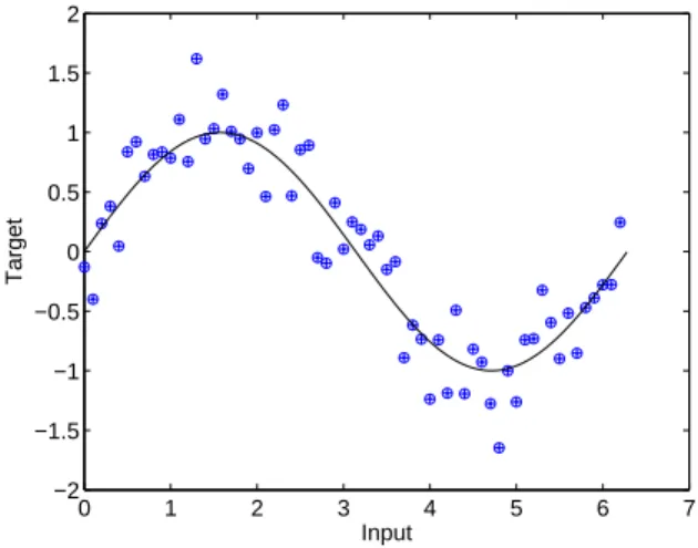
Fig. 1. Noisy sine wave training data (dots), with noiseless generating function
shown with the solid line. Noise drawn from a Gaussian with zero mean 0.3 standard deviation. 63 training data points (input values drawn at intervals of 0.1 from 0 to 2π).
3 Regularisation by multi-objective optimisation
Arguably one of the more fruitful avenues investigated so far by the EMOO community in multi-objective supervised learning is complexity model opti-misation (see e.g. [Fieldsend and Singh, 2004, Jin et al., 2004, Pappa et al., 2004] for recent work and overviews). As noted earlier, there tends to be a problem, especially when using models with high representation capability, to over-fit a model parameterisation to the training data leading to poor gen-eralisation ability. A textbook example of this would be when using neural networks (NNs). Given enough activation units NNs are universal approxima-tors, allowing sufficient complexity within the model to permit them to model any deterministic underlying generation process. However, determining the appropriate complexitya priori for a problem so as not to over-fit the data at hand is a persistent problem. As noted above, in statistical machine learning this over-fitting is typically tackled by the use of weight decay regularisation. This approach requires the determination of the regularisation parameter α on the weighting of this penalty. The use of EMOO on the other hand al-lows optimisation over all complexities. As such the problem can be cast as bi-objective for EMOO, with the first objective being the minimisation of the error function (in the regression problems shown here, the mean square error), and the second objective being the minimisation of model complexity (here, the sum of the squared weights of a multi-layer perceptron (MLP) neural network, equation 6).
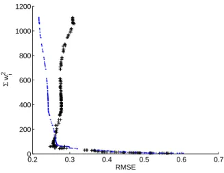
0.2 0.3 0.4 0.5 0.6 0.7 0 200 400 600 800 1000 1200 RMSE Σ w i 2
Fig. 2.Estimated Pareto optimal front of NNs (dots) and the same NNs evaluated
on a validation set from the same generation and noise process (crosses), note the switch back effect in the lower left corner.
A simple example is now provided. The problem is the regression of a noisy sine wave, using the training data illustrated in Figure 1, with circles denoting the training data and the line representing the continuous (noiseless) generating process. Using a simple greedy (1+1)–evolution strategy (ES), as described by [Fieldsend and Singh, 2002, 2005], one can discover the networks corresponding to the estimated Pareto front shown in Figure 2 with dots.
Algorithm 1 A general ‘greedy’ (1+1)–ES scheme for multi-objective op-timisation in supervised learning, where e is the set of error evaluations on model parameterisationwand data x. Error terms to be minimised without loss of generality.
Inputs:
T Number of generations
M Number of initial samples of w
1:F:=initialise(x, M) Initial estimate of front
2:fort:= 1 :T
3: w:=select(F) Select from archive
4: w′:=perturb(w) Perturb/mutate parameters
5: e:=evaluate(x,w′,)Evaluate error functions
6: F:=update(F,w′) Update archive
A general (1+1)–ES is given in algorithm 1. In the implementation of this general algorithm in this section an initial non-dominated set of points was generated by training a MLP (with one input unit, 50 hidden units and one output unit) using the quasi-Newton method [Bishop, 1995b, Nabney, 2001] and evaluating its objectives every 50 epochs, up to 5000 epochs (Algorithm 1 line 1). The ES was run for 50000 generations (line 2), with a probability of weight mutation of 0.1 and mutation being formed of additive draws from a zero mean Gaussian with standard deviation of 0.2 (line 4). In the imple-mentation hereupdate() (line 6) ensuresF always contains the best current estimate of the true Pareto front by storing an unconstrained non-dominated set of the best parameterisations found so far.
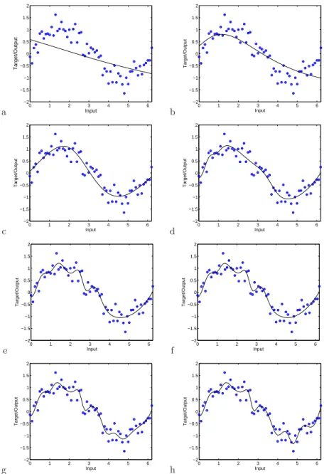
Figure 3a shows the regression lines of the model with the lowest complex-ity (summed squared weights) from the estimated Pareto front with Figures 3b-h showing the regression lines of models with consecutively higher com-plexity levels (sampled at roughly every 50th element of the estimated true Pareto front shown in Figure 2).
The models span the spectrum from severe under-fitting (such as the al-most straight lines in Figure 3a) to severe over-fitting (such as the wiggly lines shown in Figure 3h). This range of model types is to be expected from the op-timisation objectives. The problem still arises as to how to choose an operating model from the set at the end of the optimisation run. One approach discussed in [Fieldsend and Singh, 2004] is to evaluate the set on a second validation set of data and note at which point the complexity/accuracy curve ‘switches back’. This is shown in 2 by crosses, where a validation set of equal size as the training set is used, from the same noisy generating process. A prominent ‘switch back’ point can be seen in the lower left hand corner, which would lead one to either choose the model with lowest root mean squared error (RMSE) in this area, or alternatively use a equal-weighted ensemble of models from this region.
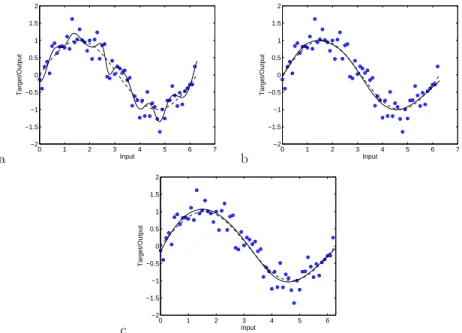
Figure 4 shows the regression line of various approaches with a solid line – in all cases the dashed line shows the underlying noiseless generating process. Figure 4a is the model with lowest RMSE on the training data (i.e., the model corresponding to the leftmost point in Figure 2), Figure 4b is the model with lowest RMSE on the validation data (i.e., the model corresponding to bottom left of the ‘switch back’ cross in Figure 2), and Figure 4c is the average regres-sion line of the 10 models with the lowest validation error (the models at the knee of the switch back). As can clearly be seen, the model with the lowest RMSE on the training data clearly is over-fitting, but the regression lines in Figures 4b and 4c are much closer to the underlying generating process. Even though the network representation capability is very high (50 hidden units, with only 63 training points) the use of a complexity minimisation objective and a validation set has led to a good estimate of the noiseless generating process. Other approaches like bootstrapping or cross validation during the optimisation itself can also be employed for a similar effect within the MOEA approach, see for instance [Fieldsend and Singh, 2005]. In addition an
inter-a 0 1 2 3 4 5 6 −2 −1.5 −1 −0.5 0 0.5 1 1.5 2 Input Target/Output b 0 1 2 3 4 5 6 −2 −1.5 −1 −0.5 0 0.5 1 1.5 2 Input Target/Output c 0 1 2 3 4 5 6 −2 −1.5 −1 −0.5 0 0.5 1 1.5 2 Input Target/Output d 0 1 2 3 4 5 6 −2 −1.5 −1 −0.5 0 0.5 1 1.5 2 Input Target/Output e 0 1 2 3 4 5 6 −2 −1.5 −1 −0.5 0 0.5 1 1.5 2 Input Target/Output f 0 1 2 3 4 5 6 −2 −1.5 −1 −0.5 0 0.5 1 1.5 2 Input Target/Output g 0 1 2 3 4 5 6 −2 −1.5 −1 −0.5 0 0.5 1 1.5 2 Input Target/Output h 0 1 2 3 4 5 6 −2 −1.5 −1 −0.5 0 0.5 1 1.5 2 Input Target/Output
Fig. 3.Regression lines of the estimated Pareto optimal NNs on the training data.
Plots (a)–(h) show models sampled regularly from estimated Pareto front, from lowest complexity to highest complexity.
a 0 1 2 3 4 5 6 7 −2 −1.5 −1 −0.5 0 0.5 1 1.5 2 Input Target/Output b 0 1 2 3 4 5 6 7 −2 −1.5 −1 −0.5 0 0.5 1 1.5 2 Input Target/Output c 0 1 2 3 4 5 6 −2 −1.5 −1 −0.5 0 0.5 1 1.5 2 Input Target/Output
Fig. 4. a) Regression line of model with lowest RMSE on training data from
esti-mated Pareto set. b) Regression line of model with lowest RMSE on validation data from estimated Pareto set (on training data). c) Regression line of ensemble of 10 models with lowest RMSE on validation data from estimated Pareto set (on training data).
esting approach to regularisation has been explored by Gr¨aning et al. [2006], who optimise Receiver Operating Characteristic performance on simulated additional training sets generated by perturbing the features of the training data with Gaussian noise.
4 Competing error terms
Another application area that has proved popular is training with multiple errors. Here conflicting ‘goodness-of-fit’ measures are used in the learning process, typically due to competing properties which are desired of the final model(s).
4.1 Regression
In the area of regression this has been in the formulation of a trade off between different measures of goodness-of-fit. For instance, using EMOO methods one may optimise with respect to one measure (e.g. RMSE or absolute error) and
also with respect to the distributional properties of this principal error mea-sure [Bi and Bennett, 2003, Fieldsend, 2006]. In the regression field EMOO methods have also been used to optimise multiple ‘application specific error terms’, for instance in financial applications the return on investment of pre-dicting an asset price. By itself is difficult to train a model using this term, but used in conjunction with a goodness-of-fit error measure can ensure that you have models that accurately predict the signal and are profitable [Fieldsend and Singh, 2002, Schlottmann and Seese, 2004].
4.2 Classification
In classification problems, the task is to allocate new or previously unseen examples x to one of two or more classes (categories) Cj. This is generally
based on a model, or set of models, induced from some existing corpus of data whose true classes are known already. The misclassification rate (proportion of data which is labelled with an incorrect class by the classifier) is typically taken as a measure of classifier accuracy, and as the objective to be minimised. However, when there is an imbalance in the number of each distinct class in a set of data, for training and/or testing, the total misclassification rate can be misleading. For instance, in a two class problem its is trivial to get a 10% misclassification rate if there is a 9:1 ratio of the two classes in the data set.
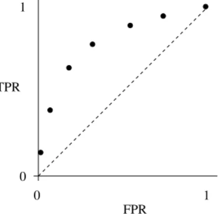
In order to deal with class imbalance Receiver Operating Characteristic Analysis (ROC) is typically used in the 2-class classifier optimisation. This analysis traces out the true positive rate (the proportion of correct assign-ments to the principal class by the model) against the false positive rate (the proportion of incorrect assignments of the second class to the principal class by the model), by varying the classification threshold of the model (if the model outputs a probability of assignment, or a score), or the parameters of the model itself. This visualisation shows the trade-off between the accuracy in classifying the two separate classes for a particular model – as illustrated in Figure 5. The best possible classifier would operate in the top left of the plot, with a TPR of one and an FPR of zero. The dashed line denotes the ran-dom allocation line, the expected performance of a classifier which allocates class labels to data at random (at some fixed ratio). Any classifier operating
below this line is performing worse than random; it can be reflected through it simply by switching the class labels it has assigned to data.
The plotting of classifier performance in the TPR/FPR plane also allows a user to evaluate models given different costs of misclassification. For example, in medical diagnosis, the cost of misclassifying a patient by saying they do not have a cancer when they do is far more costly than saying they have a cancer when they don’t. The latter error will be detected with a biopsy sample, the former error may not be detected before the cancer progresses to a more dangerous state.
The area under the ROC curve (AUC), which lies between zero and one, is often used as a single value to compare classifiers. As explained by Hand
0 0 1 1 TPR FPR
Fig. 5.ROC example. Points denote the different TPR/FPR combinations possible
from a classifier by using a different threshold on the model output (or alternatively using different model parameters).
and Till [2001], this measures a classifier’s ability to separate two classes over the range of possible costs. The Gini coefficient is also used, which is twice the area between the curve and the random allocation line.
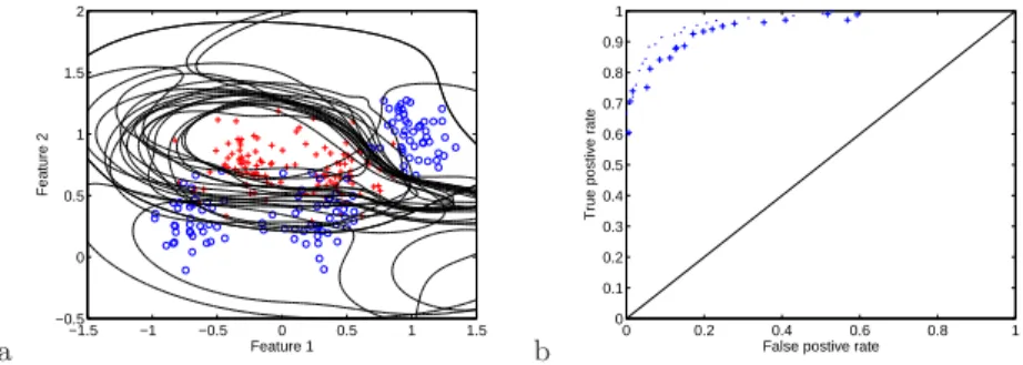
ROC analysis obviously lends itself to optimisation with EMOO meth-ods, with the TPR and FPR being cast as two separate objectives.2 The example in Figure 6a shows the decision boundaries formed by radial basis function (RBF) neural network classifiers on the test problem from [Fieldsend et al., 2003], optimised in this way using a simple (1+1)-ES.3 Figure 6b in turn shows the estimated optimal ROC curve on the 250 training data points (shown with dots on the plot), and their evaluation on 1000 testing data points (shown with crosses on the plot). Interestingly, although not shown here (but available in [Fieldsend et al., 2003]), synthetic ROC problems are perhaps the only supervised learning problems for which the true Pareto front can be determined and the performance of the optimised solutions compared to it. This is because with a synthetic classification problem one can determine the exact posterior probability of any feature vector, and therefore can trace out the ROC curve of a Bayes rule classifier (the best possible). Without knowing the generating process one cannot know where the true Pareto front lies for any classification problem, and therefore how close any particular model is to it. However, the downside to this is that when optimising a classifier based on training data, you only actually have access to an estimate of the posterior 2Alternatively one could maximise the AUC as a function of a set of solutions, if
one was careful as to how the set was updated, as discussed later.
3The RBFs contained 10 units with Gaussian kernels, optimised in the fashion discussed in [Fieldsend and Everson, 2005b] using a (1+1)-ES for 5000 generations with a probability of mutation of 0.1 and variance of additive Gaussian mutation of 0.2.
a −1.5 −1 −0.5 0 0.5 1 1.5 −0.5 0 0.5 1 1.5 2 Feature 1 Feature 2 b 0 0.2 0.4 0.6 0.8 1 0 0.1 0.2 0.3 0.4 0.5 0.6 0.7 0.8 0.9 1
False postive rate
True postive rate
Fig. 6. a) Decision contours of RBF networks on estimated optimal ROC front,
training data shown with one class denoted by circles and the other by crosses. b) Estimated optimal ROC front on 250 training data pairs ( denoted by dots) and their evaluation on 1000 testing data pairs (denoted by crosses).
probability, not the true posterior probability (otherwise you would not need a classifier in the first place). As such the estimated ROC curve may actually seemabove the known optimal curve. This problem of noise and uncertainty (which is apparent in most if not all supervised learning problems) is one of the principal areas needing additional research in multi-objective supervised learning, and can be the source of over-optimistic assessments of performance. It is also worth noting that in 2-class ROC optimisation the granularity of the front is limited by the cardinality of the dataset used – therefore uncon-strained archives may be used with a priori knowledge as to how large it is possible for them to grow.
4.3 Separating classes
An early formulation of the multi-class ROC problem was proposed by Hand and Till [2001], who introduced a generalisation of the AUC. In summary, their M measure is the average of the pairwise AUCs between theQ(Q−1)/2 pairs of classes. More precisely, Hand and Till show that the AUC is the probability, denoted ˆA(k|j),that a randomly drawn member of classCk will have a lower
estimated probability of belonging to classCj than a randomly drawn member
ofCj. Clearly a classifier which is able to separateCkfromCjhas large ˆA(k|j),
whereas if it makes assignments no better than chance ˆA(k|j) = 1/2. Except in the two class problem ˆA(k|j)= ˆ6 A(j|k), and exchanging class labels does not alter their separability, so the classifier’s ability to separate Cj and Ck is
measured by ˆA(j, k) = [ ˆA(k|j)+ ˆA(j|k)]/2.Hand and Till then define overall performance of a classifier as:
M = 2 Q(Q−1) X j<k ˆ A(j, k). (7)
Algorithm 2Evolutionary optimisation of Hand and Till’sM measure. Inputs: T Number of generations 1:E:=initialise() 2:fort:= 1 :T 3: w:=select(E)
4: w′:=perturb(w) Perturb parameters
5: ifM(E∪w′)> M(E)
6: E:=E∪w′ Insert w′
7: for u∈E
8: ifM(E) =M(E\u)
9: E:=E\u Remove redundant elements
10: end
11: end
12: end
13:end
Where Qis the number of classes. This measure thus measures the average ability of a classifier to separate classes, although it considers the pairwise performances of the classifier, rather than the full Pareto front. Hand and Till also describe the measure for a classifier with fixed parameters, rather than for a parameterised family of classifiers, as done in the next section of this chapter. A natural generalisation is to consider the multiobjective maximisation (for a parameterised family) of theQ(Q−1) pairwise ˆA(j, k). In fact, this leads to a simple algorithm for the maximisation ofM itself, which is now described. The key to maximisingMis that it is possible to find asetEof parameters w that together maximise M. Consequently if the addition of a proposed parameter vector w′ to E increases any one of the ˆA(j, k) it automatically increasesM; since an unrestricted set of parameters is kept, no other elements of E need be deleted so the other ˆA(j, k) are, at worst, not decreased. This leads to the straightforward procedure outlined in Algorithm 2. As for the multi-objective evolutionary algorithm, it maintains an archiveEof solutions. At each stage, a randomly selected member of E is perturbed and the M measure of the archive plus w′ evaluated; if the addition ofw′ increasesM thenw′ is retained (line 6 of Algorithm 2) and any parameters which now do not contribute toM are removed (lines 7-9).
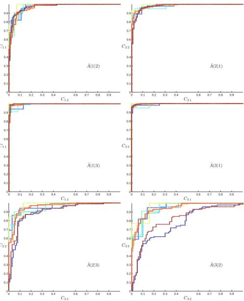
When maximising M over a family of classifiers several ROC curves for individual classifiers generally contribute to the composite ROC curve for the family. Example ROC curves for 8 classifiers resulting from the optimisation of M for synthetic data using the probabilistic k-nn classifier [Holmes and Adams, 2002] are shown in Figure 7. For each pair of classes the axes of each panel areCkk,the true positive rate forCk, andCkj,the rate at which
0 0.1 0.2 0.3 0.4 0.6 0.7 0.8 0.9 0 0.1 0.2 0.3 0.4 0.6 0.7 0.8 0.9 C1 2 C1 1 ˆ A(1|2) 0 0.1 0.2 0.3 0.4 0.6 0.7 0.8 0.9 0 0.1 0.2 0.3 0.4 0.6 0.7 0.8 0.9 C2 1 C2 2 ˆ A(2|1) 0 0.1 0.2 0.3 0.4 0.6 0.7 0.8 0.9 0 0.1 0.2 0.3 0.4 0.6 0.7 0.8 0.9 C1 3 C1 1 ˆ A(1|3) 0 0.1 0.2 0.3 0.4 0.6 0.7 0.8 0.9 0 0.1 0.2 0.3 0.4 0.6 0.7 0.8 0.9 C3 1 C3 3 ˆ A(3|1) 0 0.1 0.2 0.3 0.4 0.6 0.7 0.8 0.9 0 0.1 0.2 0.3 0.4 0.6 0.7 0.8 0.9 C2 3 C2 2 ˆ A(2|3) 0 0.1 0.2 0.3 0.4 0.6 0.7 0.8 0.9 0 0.1 0.2 0.3 0.4 0.6 0.7 0.8 0.9 C3 2 C3 3 ˆ A(3|2)
Fig. 7.Pairwise ROC curves for thek-nn classification of the 3-class synthetic data
set. Each row corresponds to a pair of classes. Axes correspond to the true positive rate Ckk and the rate at which Ck examples are misclassified as Cj. Each curve
corresponds to a distinct parameter combination, so that ˆA(k|j) is the area under the envelope of the curves.
to a distinctw={k, β}parameter value4, and the optimisedM is achieved by the envelope of these curves. Evaluation of the ˆA(k|j) that contribute to
0 500 1000 1500 2000 0.97 0.975 0.98 0.985 0.99 0.995 Iteration M m ea su re 0 500 1000 1500 2000 0 2 4 6 8 10 12 14 16 18 20 Iteration Archive size
Fig. 8. Left: Growth ofM with iteration during optimisation. Right: Number of
distinct parameter combinations contributing toMduring optimisation. Results for
k-nn classification of 3-class synthetic data.
M can be performed by applying the method described by Hanley and McNeil [1982] and Hand and Till [2001, page 174] for calculating the AUC for a single classifier to the envelope of the ROC curves.
As Figure 7 shows, after optimisation only 8 distinct (k, β) combinations contribute to the optimised M ≈0.991, although during optimisation up to 20 parameter combinations were involved. Selection of the operating param-eters on the basis of the ˆA(j, k) is possible, it is emphasised that the ˆA(j, k) summarise the overall pairwise separability rather than permitting specific choices to be made between particular misclassification rates. Additional in-formation is available through examination of the families of pairwise tradeoff curves such as those displayed in Figure 7.
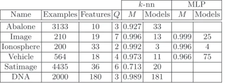
As the optimisedMmeasures the ability of a particular family of classifiers to separate classes, it may be used for comparing classifiers. Table 1 shows the optimised M and number of distinct models (distinct parameter values) contributing toM for a number of standard machine learning data sets taken from the UCI repository [Blake and Merz, 1998]. The two-class Ionosphere data is well known to be easily classified and M (actually the AUC here) is correspondingly high with only 3 distinct parameter sets for thek-nn classifier and 4 sets for the MLP. The Image data can be well separated, but only with the use of 13 parameter sets fork-nn; again better separation is achieved by the more flexible MLP, but at the expense of many more models. The DNA data with only 3 classes but 180 features requires 181 (k, β) combinations for optimal separation. In contrast, even after optimisation the Satimage data cannot be well separated withk-nn classifiers. Results are not presented for the MLP classification of the Abalone, Satimage and DNA datasets because the computation of the ˆA(j|k) for envelopes of individual classifiers becomes exorbitantly expensive with many samples and models.
Table 1.OptimisedM measure for UCI data sets.
k-nn MLP
Name Examples Features Q M Models M Models Abalone 3133 10 3 0.927 33 Image 210 19 7 0.996 13 0.999 25 Ionosphere 200 33 2 0.992 3 0.996 4 Vehicle 564 18 4 0.973 11 0.966 75 Satimage 4435 36 6 0.713 20 DNA 2000 180 3 0.989 181
In summary, althoughM provides a global measure of a classifier’s per-formance on a particular dataset and identifies a relatively small number of optimal parameter sets, the question of how to select an operating point re-mains. The question arises for instance, whether a single operating point se-lected from a group which together maximisesM would necessarily be as good as a single operating point maximised for M. In the next section a different approach to multi-class ROC optimisation is discussed which confronts some of these issues.
4.4 Multi-class ROC
The authors have shown recently that with Q-classes (where Q > 2) ROC analysis can be extended and cast in terms of minimising the off-diagonal elements of the confusion rate matrix [Fieldsend and Everson, 2005b, Everson and Fieldsend, 2006a,b]. An example confusion rate matrix is given below – note here the true positive rates and false positive rates are not available as such, but class assignment rates (where Ci,j/|Ci|denotes the classification
rate of classi data to classj, normalised by the total number of classidata points). Predicted Class 1 2 . . . 3 1 C1,1 |C1| C1,2 |C1| . . . C1,Q |C1| Actual Class 2 C2,1 |C2| C2,2 |C2| . . . C2,Q |C2| . . . . Q CQ,1 |CQ| CQ,2 |CQ| . . . CQ,Q |CQ|
This is therefore a Q(Q−1) objective minimisation problem. However, although the dimensionality of the Pareto front/optimal ROC front increases rapidly with the number of classes, like the 2-class problem, there is a limit to the number of distinct points on it which is a function of the size of the data set used, andQ(albeit potentially very large).
By extending the Gini coefficient analysis a random allocation simplex can be used to compare different classifiers inQ(Q−1) dimensional objective space. Classifiers whose off-diagonal confusion rates sum to greater thanQ−1 are performing worse than average. Additionally that single model, which is furthest in front of this simplex (closest to the origin) should be the classifier chosen when no misclassification costs are known (for a more extensive discus-sion see [Everson and Fieldsend, 2006b]). This also allows the comparison of different classifiers families for particular supervised learning problems (e.g.
k-nearest neighbour classifiers, decision trees, multi-layer perceptrons, radial basis functions, etc.). Using this the comparison can concern itself not simply with the cardinality of dominance between the points on the ROC front pro-duced, but also using a measure on the objective space which is meaningful (similar to the volume measure, or S metric, used in general multi-objective optimisation, but without scaling – and based on a pre-specified region of a hypercube). More formally, [Everson and Fieldsend, 2006b] have shown that the volume lying between the origin (the perfect classifier) and the random allocation simplex, that also lies in the unit hypercube (where it is feasible for a classifier performing better that average to operate) is:
(Q−1)Q(Q−1) (Q(Q−1))! −
Q(Q−1)(Q−2)Q(Q−1)
(Q(Q−1))! . (8)
This region is denoted here byP. The measure on it,G(), is calculated as the proportion ofPdominated by elements of the ROC surface (F). Therefore, like the Gini coefficient in two dimensions, G(F) is a measure of how much better than random the elements in a set F are. δ(F, F′) in turn measures how much ofP is dominated by the setF but not by the setF′. This can be used to compare two different fronts (for instance generated by two different classifier families) which possibly overlap in parts.
Due to the shape of the region, it is not quite as trivial to calculate its volume as it is to calculate the region used in the S metric [Zitzler, 1999], as a reference simplex is used as opposed to a reference point (and this is further constrained to lie within a unit hypercube). As such the region defined by P is a hyper-pyramid, with aQ(Q−1) truncated corners. Monte Carlo sampling of this region can give a good estimate of the volume dominated however, and [Fieldsend, 2005] discusses how to do this efficiently.5
When using a soft classifier (one that gives a probability of class member-ship, or a score) it is computationally efficient to assess the effect of a number 5If the reader is considering using this measure to compare multi-class ROC curves they are strongly advised to consult this technical report, as the probability of randomly generating a sample in the region defined byP, by generating a Uni-form sample in the unit hypercube, is (Q−1)Q(Q−1)
(Q(Q−1))! −
Q(Q−1)(Q−2)Q(Q−1)
(Q(Q−1))! , which rapidly becomes become prohibitively small at even small Q. Sampling methods developed in [Fieldsend, 2005] generate random points inP with a probability of
≈ 1
Algorithm 3 Converting the general (1+1)–ES scheme for multi-objective optimisation in supervised learning (Algorithm 1), into a (1+λ) scheme for ROC optimisation (replacing lines 7 and 8 of original algorithm).
Inputs:
λ Number of cost samples
1: forj:= 1 :λ
2: c:=sample() sample costs
3: e:=evaluate(x,w′,c) Evaluate error functions
4: F:=update(F,w′,c) Update archive
5: end
of different sample cost matrices,c, on the misclassification rates for any par-ticular model parameterisation.6This is because passing the data,x, through a classification model can be time consuming, whist transforming this output using different cost matrices allows the evaluation of many different possible misclassification combinations relatively cheaply. As such the imposition of Algorithm 1 is better viewed as a (1 +λ)–ES, withλcost matrices, c, addi-tionally sampled for any particular model parameterisation,w.7As such lines 7 and 8 of Algorithm 1 should be replaced by Algorithm 3.
In the empirical results given below λ = 50 different cost matrices are assessed for each model parameterisation, drawn from unbiased Dirichlet dis-tributions, with each optimisation run lastingT = 5000 generations (therefore 5000 unique model parameterisations evaluated, each with 50 different cost matrices). Probability of parameter mutation was 0.8, with the mutation being additive draws from a Gaussian distribution with zero mean and 0.2 standard deviation.
Results are given here for the UCI Image, Vehicle and Satimage data sets. Details of data set sizes are given in Table 1, and therefore the objective dimensionality for these sets in this problem formulation are 42, 12 and 30 re-spectively. The classification models used are the probabilistick-nn algorithm, probabilistic k-nn algorithm with tricube kernel [Holmes and Adams, 2002] and the multinomial logistic regression classifier (MLR) [Bishop, 1995a]. The probabilistick-nn classifier is a simplelocal classifier which classifies based on the actual classes of known data in the unlabelled data’s immediate locality. It has two parameters,k, the number of neighbours used andβ, which controls the ‘strength of association’ between neighbours (effectively a way of mak-ing closer neighbours more important). The MLR is a simpleglobal classifier which separates feature space into different classes with smooth planes, and has D(Q+ 1) parameters (where D is the number of features – the size of x). The probabilistic k-nn with a tricube kernal has the local classification
6Assuming linear costs.
7These sample costs can be straightforwardly and randomly sampled from a Dirich-let distribution, see [Everson and Fieldsend, 2006b] for a discussion on this.
Image −1 −0.9 −0.8 −0.7 −0.6 −0.5 −0.4 −0.3 0 500 1000 1500 2000 2500 3000
Signed distance from random allocation simplex
Number of solutions −10 −0.9 −0.8 −0.7 −0.6 −0.5 −0.4 −0.3 500 1000 1500 2000 2500 3000 3500
Signed distance from random allocation simplex
Number of solutions −1 −0.9 −0.8 −0.7 −0.6 −0.5 −0.4 −0.3 0 200 400 600 800 1000 1200 1400
Signed distance from random allocation simplex
Number of solutions Vehicle −1 −0.9 −0.8 −0.7 −0.6 −0.5 −0.4 −0.3 0 100 200 300 400 500 600 700 800 900 1000
Signed distance from random allocation simplex
Number of solutions −10 −0.9 −0.8 −0.7 −0.6 −0.5 −0.4 −0.3 500 1000 1500 2000 2500
Signed distance from random allocation simplex
Number of solutions −1 −0.9 −0.8 −0.7 −0.6 −0.5 −0.4 −0.3 0 100 200 300 400 500 600
Signed distance from random allocation simplex
Number of solutions Satimage −1 −0.9 −0.8 −0.7 −0.6 −0.5 −0.4 −0.3 0 200 400 600 800 1000 1200 1400 1600
Signed distance from random allocation simplex
Number of solutions −10 −0.9 −0.8 −0.7 −0.6 −0.5 −0.4 −0.3 200 400 600 800 1000 1200 1400 1600 1800
Signed distance from random allocation simplex
Number of solutions −1 −0.9 −0.8 −0.7 −0.6 −0.5 −0.4 −0.3 0 50 100 150 200 250 300 350 400 450 500
Signed distance from random allocation simplex
Number of solutions
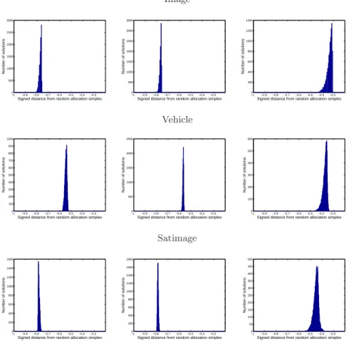
Fig. 9.Distances from the random classifier simplex. Negative distances correspond
to models inP.Left: k-nn;Middle: k-nn tricube.Right:MLR.Top:UCI Image data;
Middle:UCI Vehicle data;Bottom: UCI Satimage data.
properties of the probabilistick-nn, with an additional tendency to push the assignment probability down if the unlabelled sample is ‘far’ from any labelled data.
Figure 9 shows the signed distance of all points lying on the ROC curve for each classifier from the random allocation simplex – negative numbers mean the operating point is better than random and a value of -1 indicates that the model perfectly classifies the data presented. As can be seen, visually both variants of the probabilistick-nn classifier seem to do considerably better than the MLR classifier, with all classifiers performing better than random. Table 2 provide the associated G and δ measures, calculated from 10000 Monte Carlo samples in P. From these it can be seen that for the Image dataset the probabilistick-nn model would tend to be the preferred model, with only
Table 2. Generalised Gini coefficients and exclusively dominated volume compar-isons of the probabilistic k-nn, probabilistic k-nn with tricube kernel and MLR classifiers.
Measure Image Vehicle Satimage G(k-nn) 0.137 0.073 0.116 G(k-nn tricube) 0.080 0.030 0.099 G(MLR) ≈0 0.009 ≈0 δ(k-nn, k-nn tricube) 0.070 0.044 0.026 δ(k-nn,MLR) 0.137 0.068 0.116 δ(k-nn tricube, k-nn) 0.013 0.001 0.008 δ(k-nn tricube,MLR) 0.080 0.028 0.099 δ(MLR, k-nn) 0 0.005 0 δ(MLR, k-nn tricube) 0 0.007 0
small portions of its front lying behind that of the probabilistick-nn tricube model (additionally the probabilistick-nn model has the single operating point furthest from the random allocation simplex). A similar result can be seen for the Vehicle data set, although here it is interesting to note that, although the MLR visually seems to under perform compared to the k-nn models, the δ measures show that, for some particular choices of costs, the MLR classifier is actually the best to choose. The results from the Satimage dataset again give the same overall order on the classifiers, with the MLR being totally worse, irrespective of costs, than both types of probabilistick-nn model. Again, for some cost combinations the model with the tricube kernel is a better classifier to use; however for the majority of costs preferences the standard probabilistic
k-nn is the most appropriate classifier to choose of the three model families compared.
Compared to optimising using the M measure a far larger range of pa-rameters is found to be optimal under this framework. For instance, when using the probabilistic k-nn model for the synthetic data in Section 4.3, 8 different parameterisations described the set which maximised M, compared to approximately 7500 solutions on the Pareto optimal ROC surface for the same dataset described in [Everson and Fieldsend, 2006b]. The Pareto opti-mal ROC surface, however, describes the full range of trade-offs that may be obtained between classification rates, rather than the average class separa-bility over the range of pairwise cost ratios described byM, and also shows the user which cost matrix (equivalent to threshold in 2 class cases) is needed to use with a model parameterisation to obtain a particular expected set of misclassification rates.
5 Discussion
There are a number of other avenues in multi-objective supervised learning which have been explored using EMOO (for instance ensemble training, which is the subject of another chapter in this book), the examples presented here present a reasonable overview of the area, with a focus on the new area of multi-class ROC optimisation. A more general overview can also be found in [Jin, 2006].
However, there are still a large number of open questions in the field of multi-objective supervised learning that are worth highlighting:
Hybrid models:
Usually researchers tend to either start a process with a ‘traditional’ local optimiser (like gradient descent in NNs), or iterate between a local process and an EMOO method. This tends to be because the search space is easier traversed (at least to begin with) by local methods, and because, for many of the classifiers/regressors used, the range of parameters to be searched is essentially without limits. As such EMOO techniques are often used to trace out an estimate of the Pareto front for a problem after a traditional algorithm has supplied a single point on a good estimate of the front. The question of how much search to carry out with local methods and how much time to spend searching with EMOO methods is still an open one.
Over-fitting:
Unless there is an explicit casting of an objective to minimise complexity, EMOO approaches to optimising competing errors can be very prone to over-fitting. The use of weight decay regularisation approaches in hybrid EMOOs may mitigate this somewhat – but to do this they must assume a penalty term independent of the region of objective space, which is a difficult assumption to justify.
Many to one mappings:
Perhaps more than other application areas, supervised learning parameter space is full of regions which have identical evaluations in objective space – especially if it is a classification problem. These disjoint plateaus can cause many problems for optimisers, and when using an elite multi-objective opti-miser raises the question as to which solution to store if they have the same objective valuations but very different input space partitioning. Figure 10 illustrates this with the synthetic classification problem used earlier – the de-cision contours shown have identical misclassification rates on the data, but have different decision boundaries.
−1.5 −1 −0.5 0 0.5 1 1.5 −0.5 0 0.5 1 1.5 2 Feature 1 Feature 2
Fig. 10.Example decision boundaries (from RBF classifiers) with identical
operat-ing points in ROC space.
Noise, uncertainty, truth:
Arguably the largest problem in multi-objective supervised learning is the fact that only samples of the generating process are available, which tend to be noisy. Optimising with uncertainty/robust optimisation is an area which is gaining more interest in the general EMOO community at the current time [Hughes, 2001, Teich, 2001, Fieldsend and Everson, 2005a, Goh and Tan, 2006] and supervised learning problems should present an interesting avenue of re-search. Given the concerns of data mis-labelling or feature/sensor noise, and the uncertainty caused when many different models/model parameterisations can lead to the same objective evaluation (on a certain data sample), as men-tioned above, all supervised learning problems seem to contain at least one form of uncertainty.
6 Acknowledgements
The authors would like to thank Michelle Fisher for helpful comments during the development of this chapter, and the anonymous reviewers who helped considerably in its improvement.
References
J. Bi and K.P. Bennett. Regression Error Characteristic Curves. In Pro-ceedings of the Twentieth International Conference on Machine Learning (ICML-2003), pages 43–50, Washington DC, 2003.
C. Bishop.Neural Networks for Pattern Recognition. Clarendon Press, Oxford, 1995a.
C.M. Bishop. Neural Networks for Pattern Recognition. Oxford University Press, 1995b.
C.L. Blake and C.J. Merz. UCI repository of machine learning databases, 1998. URLhttp://www.ics.uci.edu/∼mlearn/MLRepository.html. R. O. Duda, P. E. Hart, and D. G. Stork. Pattern Classification.
Wiley-Interscience Publication, 2000.
R.M. Everson and J.E. Fieldsend. Multi-objective optimization of safety re-lated systems: An application to short term conflict alert. IEEE Transac-tions on Evolutionary Computation, 10(2):187–198, 2006a.
R.M. Everson and J.E. Fieldsend. Multi-class roc analysis from a multi-objective optimisation perspective. Pattern Recognition Letters, 2006b. J.E. Fieldsend. Regression error characteristic optimisation of non-linear
mod-els. In Yaochu Jin, editor,Multi-Objective Machine Learning, volume 16 of
Studies in Computational Intelligence, pages 103–123. Springer, 2006. J.E. Fieldsend. A short note on the efficient random sampling of the
multi-dimensional pyramid between a simplex and the origin lying in the unit hypercube. Technical Report 419, Department of Computer Science, Uni-versity of Exeter, August 2005.
J.E. Fieldsend and R.M. Everson. Multi-objective optimisation in the presence of uncertainty. InProceedings of the 2005 IEEE Congress on Evolutionary Computation (CEC’05), pages 476–483, 2005a.
J.E. Fieldsend and R.M. Everson. Formulation and comparison of multi-class roc surfaces. InProceedings of the 2nd ROCML workshop, part of the 22nd International Conference on Machine Learning (ICML 2005), pages 41–48, 2005b.
J.E. Fieldsend and S. Singh. Pareto multi-objective non-linear regression modelling to aid capm analogous forecasting. In Proceedings of the IEEE International Joint Conference on Neural Networks, pages 388–393, 2002. J.E. Fieldsend and S. Singh. Pareto evolutionary neural networks. IEEE
Transactions on Neural Networks, 16(2):338–354, 2005.
J.E. Fieldsend and S. Singh. Optimizing forecast model complexity using multi-objective evolutionary algorithms. In C.A.C Coello and G.B. Lam-ont, editors,Applications of Multi-Objective Evolutionary Algorithms, pages 675–700. World Scientific, 2004.
J.E. Fieldsend, T.C. Bailey, R.M. Everson, W.J. Krzanowski, D. Partridge, and V. Schetinin. Bayesian inductively learned modules for safety critical systems. InProceedings of the 35th Symposium on the Interface: Computing Science and Statistics, pages 110–125, 2003.
C.K. Goh and K.C. Tan. Noise handling in evolutionary multi-objective opti-mization. Inroceedings of the 2006 IEEE Congress on Evolutionary Com-putation (CEC’06), 2006.
L. Gr¨aning, Y. Jin, and B. Sendhoff. Generalization improvement in multi-objective learning. In2006 International Joint Conference on Neural Net-works, pages 9893–9900, 2006.
D.J. Hand and R.J. Till. A simple generalisation of the area under the ROC curve for multiple class classification problems. Machine Learning, 45:171– 186, 2001.
J.A. Hanley and B.J. McNeil. The meaning and use of the area under a receiver operating characteristic (ROC) curve. Radiology, 82(143):29–36, 1982.
C.C. Holmes and N.M. Adams. A probabilistic nearest neighbour method for statistical pattern recognition.J. Royal Statistical Society B, 64:1–12, 2002. E.J. Hughes. Evolutionary multi-objective ranking with uncertainty and noise. In Evolutionary Multi-Criterion Optimization, EMO 2001, LNCS 1993, pages 329–342, 2001.
Y. Jin, editor. Multi-objective Machine Learning. Springer, 2006.
Y. Jin, T. Okabe, and B. Sendhoff. Evolutionary multi-objective optimiza-tion approach to constructing neural network ensembles for regression. In C.A.C Coello and G.B. Lamont, editors, Applications of Multi-Objective Evolutionary Algorithms, pages 653–673. World Scientific, 2004.
Y. LeCun, J. Denker, S. Solla, R.E. Howard, and L.D Jackel. Optimal brain damage. In D.S. Touretzky, editor,Advances in neural information process-ing systems II. Morgan Kaufmann, 1990.
D. J. C. MacKay. Bayesian interpolation.Neural Computation, 4(3):415–447, 1992a.
D. J. C. MacKay. A practical Bayesian framework for backpropagation net-works. Neural Compuation, 4(3):448–472, 1992b.
I.T. Nabney. Netlab: Algorithms for Pattern Recognition. Springer-Verlag, 2001.
G.L. Pappa, A.A. Freitas, and C.A.A. Kaestner. Multi-objective algorithms for attribute selection in data mining. In C.A.C Coello and G.B. Lam-ont, editors,Applications of Multi-Objective Evolutionary Algorithms, pages 603–626. World Scientific, 2004.
F. Schlottmann and D. Seese. Financial applications of multi-objective evo-lutionary algorithms: recent developments and future research directions. In C.A.C Coello and G.B. Lamont, editors,Applications of Multi-Objective Evolutionary Algorithms, pages 627–652. World Scientific, 2004.
J. Teich. Pareto-front exploration with uncertain objectives. In Evolution-ary Multi-Criterion Optimization, EMO 2001, LNCS 1993, pages 314–328, 2001.
J. Utans and J. Moody. Selecting neural network architectures via the predic-tion risk: applicapredic-tion to corporate bond rating predicpredic-tion. InProceedings of the First International Conference on AI applications on Wall Street, pages 35–41, 1991.
D. Wolpert. On bias plus variance. Neural Computation, 9(6):1211–1243, 1997.
E. Zitzler. Evolutionary Algorithms for Multiobjective Optimization: Methods and Applications. PhD thesis, Swiss Federal Institute of Technology (ETH), Zurich, Switzerland, 1999.