METRIC LEARNING FOR INCORPORATING
PRIVILEGED INFORMATION IN
PROTOTYPE-BASED MODELS
by
SHEREEN FOUAD
A thesis submitted to
The University of Birmingham
for the degree of
DOCTOR OF PHILOSOPHY
School of Computer Science
College of Engineering and Physical Sciences
The University of Birmingham
University of Birmingham Research Archive
e-theses repositoryThis unpublished thesis/dissertation is copyright of the author and/or third parties. The intellectual property rights of the author or third parties in respect of this work are as defined by The Copyright Designs and Patents Act 1988 or as modified by any successor legislation.
Any use made of information contained in this thesis/dissertation must be in accordance with that legislation and must be properly acknowledged. Further distribution or reproduction in any format is prohibited without the permission of the copyright holder.
To my beloved sister
Abstract
Prototype-based classification models, and particularly Learning Vector Quantization (LVQ) frameworks with adaptive metrics, are powerful supervised classification techniques with good generalization behaviour. This thesis proposes three advanced learning methodologies, in the context of LVQ, aiming at better classification performance under various classification settings. The first contribution presents a direct and novel methodology for incorporating valuable privileged knowledge in the LVQ training phase, but not in testing. This is done by manipulat-ing the global metric in the input space, based on distance relations revealed by the privileged information. Several experiments have been conducted that serve as illustration, and demon-strate the benefit of incorporating privileged information on the classification accuracy.
Subsequently, the thesis presents a relevant extension of LVQ models, with metric learning, to the case of ordinal classification problems. Unlike in existing nominal LVQ, in ordinal LVQ the class order information is explicitly utilized during training. Competitive results have been obtained on several benchmarks, which improve upon standard LVQ as well as benchmark ordinal classifiers.
Finally, a novel ordinal-based metric learning methodology is presented that is principally intended to incorporate privileged information in ordinal classification tasks. The model has been verified experimentally through a number of benchmark and real-world data sets.
Acknowledgements
First of all, I would like to express my deepest thanks to my supervisor, Dr. Peter Tino, who provided me with a substantial support from the beginning of my PhD all the way to the end. I appreciate Dr. Peter Tino’s continuous encouragement, careful supervision and constructive guidance on how the PhD research could be pushed further and improved upon.
I would like to thank my Thesis Group Members, Dr. John Bullinaria (RSMG rep) and Dr. Ata Kaban, who have given time, thoughts and interesting research ideas about this thesis development.
I am also grateful to Dr. Somak Raychaudhury who allowed me to benefit from his valuable knowledge and experience in the field of astrophysics during our research collaboration.
Many thanks go to Dr. Petra Schneider for our research collaboration and for providing me with the preliminarily material needed in the first part in my research.
Special thanks go to the Islamic Development Bank (IDB) who granted me a generous financial and moral support throughout my PhD scholarship.
The completion of this thesis would have been impossible, without the support and encour-agement from my beloved husband Ahmed, I will remain indebted for you forever. My lovely boys Aly and Omar, thank you for being so supportive, understanding and patient with me in the past four years. Mom, Dad, mother and father in law thank you for your continued and unconditional support. My dear brother Taha, I owe my deepest gratitude to you.
Contents
1 Introduction 1
1.1 Motivation . . . 3
1.2 Contributions . . . 4
1.3 Thesis Outline . . . 6
1.4 Publications From the Thesis . . . 8
2 Prototype-Based Learning Models 9 2.1 Introduction . . . 9
2.2 Nearest Prototype Classification . . . 11
2.2.1 Learning Vector Quantization (LVQ) . . . 13
2.2.2 Generalized LVQ (GLVQ) . . . 15
2.3 LVQ with Adaptive Metrics . . . 17
2.3.1 Relevance LVQ (RLVQ) . . . 17 2.3.2 Generalized Relevance LVQ (GRLVQ) . . . 18 2.3.3 Matrix LVQ (MLVQ). . . 19 2.3.4 Generalized Matrix LVQ (GMLVQ) . . . 20 2.4 Research Questions . . . 24 2.5 Chapter Summary . . . 26
3 Incorporating Privileged Information Through Metric Learning 27 3.1 Introduction . . . 27
3.2 Learning Using Privileged Information (LUPI) . . . 29
3.3 Distance Metric Learning (DML). . . 34
3.3.1 Information Theoretic Metric Learning (ITML) . . . 36
3.4 LUPI in the Prototype-Based Model GMLVQ . . . 40
3.4.1 Metric Fusion (MF) Approach . . . 40
3.4.2 Information Theoretic (IT) Approach . . . 45
3.5 Incorporating Privileged Information in Classifiers . . . 48
3.5.1 Transformed Basis (TB) . . . 48
3.5.2 Extended Model (Ext) . . . 50
3.6 Computational Complexity Analysis . . . 50
3.7 Experiments and Evaluations . . . 51
3.7.2 Comparison with SVM and SVM+ . . . 57
3.7.3 Galaxy Morphological Classification using Full Spectra as Privileged Information . . . 67
3.8 Discussion. . . 71
3.9 Chapter Summary . . . 73
4 Adaptive Metric Learning Vector Quantization for Ordinal Classification 75 4.1 Introduction . . . 75
4.2 Ordinal Classification Related Work . . . 77
4.3 The Proposed Ordinal LVQ Classifiers . . . 80
4.3.1 Identification of Class Prototypes to be Adapted. . . 81
4.3.2 Prototype Weighting Scheme. . . 83
4.3.3 Ordinal MLVQ (OMLVQ) Algorithm . . . 85
4.3.4 Ordinal GMLVQ (OGMLVQ) Algorithm . . . 87
4.4 Experiments and Evaluations . . . 91
4.4.1 Comparison with MLVQ and GMLVQ . . . 96
4.4.2 Comparison with Benchmark Ordinal Regression Approaches . . . 98
4.4.3 Sensitivity of the Ordinal LVQ Models to the Correct Region. . . 101
4.5 Discussion. . . 104
4.6 Chapter Summary . . . 105
5 Ordinal-Based Metric Learning for Learning Using Privileged Information 111 5.1 Introduction . . . 111
5.2 Metric Learning for Ordinal Prediction . . . 113
5.3 Ordinal-Based Information Theoretic (OIT) for Incorporating Privileged Infor-mation . . . 114
5.3.1 (Dis)similarity Constraints Derivation . . . 115
5.3.2 Weighting Scheme for the Metric Learning . . . 115
5.3.3 Ordinal-Based Metric Learning Algorithm . . . 117
5.4 Incorporating Privileged Information Into the OGMLVQ . . . 118
5.5 Experiments and Evaluations . . . 120
5.5.1 Controlled Experiments on Benchmark Data Sets . . . 122
5.5.2 Galaxy Morphological Ordinal Classification Using Spectra as Privi-leged Information. . . 124
5.5.3 Real-world Ordinal Time Series Predictions . . . 127
5.6 Discussion. . . 138
5.7 Chapter Summary . . . 141
6 Conclusions and Future Work 143 6.1 Conclusion . . . 143
A Description of Experimental Setup 149
A.1 Experimental Setup for Chapter Three Experiments . . . 149
A.2 Experimental Setup for Chapter Four Experiments. . . 150
A.3 Experimental Setup for Chapter Five Experiments . . . 153
List of Figures
3.1 Illustration of the process of finding minimizer of the cost function I con-strained on the manifoldMof symmetric positive definite matrices. . . 44
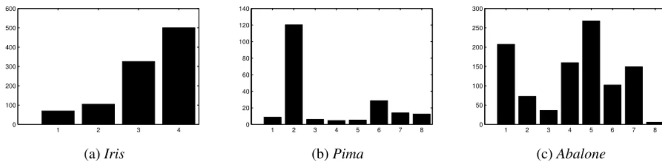
3.2 Visualization of the diagonal elements of the GMLVQ relevance matrix Λ in
Iris,PimaandAbalonedata sets shown in (a),(b) and (c), respectively. . . 55
3.3 Illustration of the rescaled MNISTdigits of ’5’ and ’8’, from 28×28 to 10×10 pixels. The later case is used in experiments. . . 58
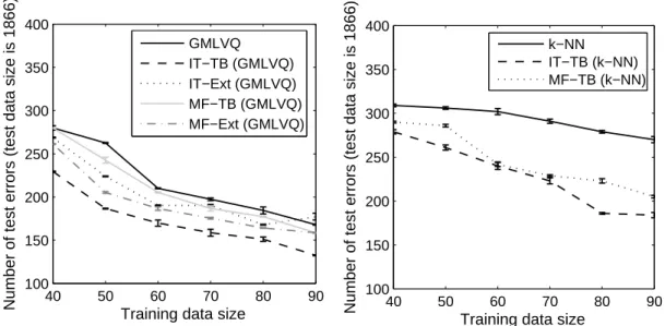
3.4 Number of misclassified points obtained by GMLVQ (left figure) and k-NN (right figure) classifications (error bars report standard deviation across 12 train-ing re-sampltrain-ing) conducted on theMNISTdata set (images ’5’ and ’8’). . . 59
3.5 Number of misclassified points obtained by the IT-TB in GMLVQ and the pre-viously introduced SVM+ based models for LUPI conducted on theMNISTdata set (images ’5’ and ’8’). . . 60
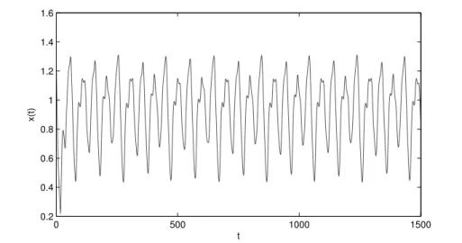
3.6 1500 points inMackey-Glass time series. . . 61
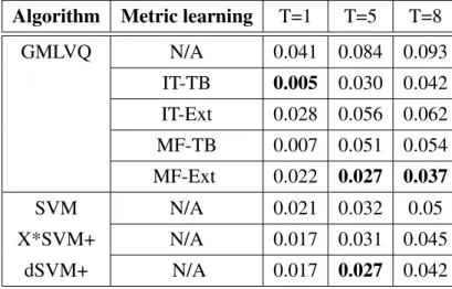
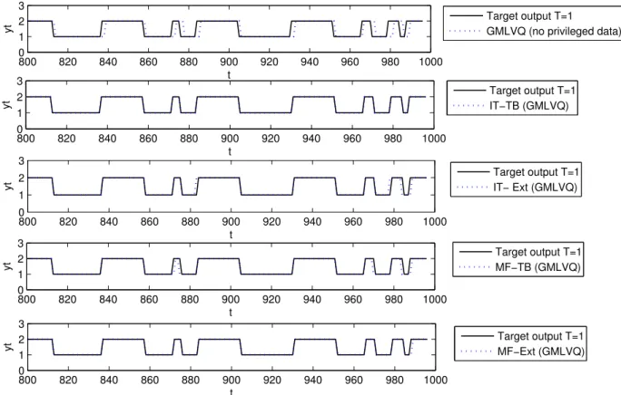
3.7 Predicted output time series (dashed line) vs. Target output time series (solid line) for (T=1) in the interval from t=800 to t=1000 in the test set, obtained by the different learning algorithms. . . 64
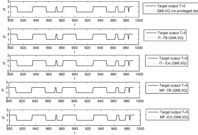
3.8 Predicted output time series (dashed line) vs. Target output time series (solid line) for (T=5) in the interval from t=800 to t=1000 in the test set, obtained by the different learning algorithms. . . 65
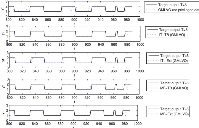
3.9 Predicted output time series (dashed line) vs. Target output time series (solid line) for (T=8) in the interval from t=800 to t=1000 in the test set, obtained by the different learning algorithms. . . 66
3.10 Galaxy Morphological classes in the Hubble’s Original Tuning Fork Diagram . 67
3.11 Visualization of the diagonal elements of the GMLVQ relevance matrix Λ in the 40 selected spectra features.. . . 69
3.12 Mean misclassification rates (error bars report standard deviation across 10 training/test re-sampling) obtained using varying amounts of privileged infor-mation. . . 72
4.1 Correct and incorrect prototype classes estimation. Given training patternc(xi) = 2indicated with square, and thresholdLmin = 1. White circles are prototypes
of correct classes with respect toc(xi), while black circles indicate prototypes
4.2 Illustrative example for one training iteration in the proposed ordinal LVQ train-ing algorithm. . . 84
4.3 MZE results for the eight benchmark ordinal regression data sets.. . . 96
4.4 MAE results for the eight benchmark ordinal regression data sets. . . 97
4.5 MZE, MAE and MMAE results for the the two real-world ordinal regression data sets shown in (a), (b) and (c), respectively. . . 98
4.6 Ordinal prediction results of a single example run inMachineCpudata set (true labels in (a)) obtained by MLVQ, OMLVQ, GMLVQ and OGMLVQ shown in (b),(c),(d) and (e), respectively. . . 107
4.7 Ordinal prediction results of a single example run in Bostondata set (true la-bels in (a)) obtained by MLVQ, OMLVQ, GMLVQ and OGMLVQ shown in (b),(c),(d) and (e), respectively. . . 108
4.8 Visualizations of ordinal predication results obtained by GMLVQ (a) and OGM-LVQ (b) of a single example run onAbalonetest set with respect to two domi-nant dimensions (using PCA). . . 109
4.9 Evolution of MAE in the course of training epochs (t) in the Abalonetraining set obtained by the MLVQ, OMLVQ algorithms, in (a) and (b), respectively. . . 109
4.10 Evolution of MAE in the course of training epochs (t) in theBostontraining set obtained by the GMLVQ, OGMLVQ algorithms, in (a) and (b), respectively. . . 110
5.1 TheSanta Fe Lasertime series set. . . 128
5.2 Histogram of the difference between the successive laser activation. Dotted ver-tical lines show the cut valuesΘ1 =−56andΘ1 = 56, while solid vertical line shows the cut valueΘ3 = 0. Ordinal symbols corresponding to the quantized regions appear on the top of the figure. . . 130
5.3 TransformedSanta Fe Lasertime series (ordinal symbols). . . 130
5.4 Predicted output time series (black line) vs. Target output time series (Grey line) in the interval from t=0 to t=5000 on the test set, obtained by the OGM-LVQ (trained onX only, without privileged data) and the two best performing learning algorithms (OIT-TB and OIT-Ext) for LUPI. The black lines in the figure indicate mistakes in predictions. . . 132
5.5 TheAustralian red-winesales (in kiloliters) from January 1980 - October 1991. 133
5.6 Histogram of the difference between thered-winemonthly sales values. Dotted vertical lines show the cut values Θ1 = −450 and Θ2 = 350, while solid vertical line shows the cut valueΘ3 = 50. Ordinal symbols corresponding to the quantized regions appear on the top of the figure. . . 134
5.7 TransformedAustralian red-wineMonthly Sales series (ordinal symbols). . . . 134
5.8 Fish Recruitmenttime series (number of new fishes) over the period 1950-1987. 136
5.9 Histogram of the difference between theFish Recruitmentnumbers. Dotted and solid vertical lines shows the cut valuesΘ1 = −11and Θ1 = 12, while solid vertical line shows the cut valueΘ3 = 0. Ordinal symbols corresponding to the quantized regions appear on the top of the figure. . . 137
List of Tables
3.1 Summary of models constructed within the LUPI for classification framework. 53
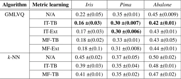
3.2 Mean misclassification rates for GMLVQ andk-NN classifications, along with standard deviations (±) across 10 training/test re-sampling, obtained on Iris,
Pima, and Abalone data sets. Each training point has both the original and privileged information. The best results are marked with bold font. . . 56
3.3 Results of statistical test (p-values of the one-sided Sign Test) comparing the standard GMLVQ and k-NN against their counterparts with LUPI, across 10 training/test re-sampling, obtained onIris,Pima, andAbalonedata sets. Statis-tically significant results withp-values<0.05 are marked with bold font. . . 56
3.4 Mean misclassification rates for GMLVQ classification (using the Transformed Basis scenario only), along with standard deviations (±) across 10 training/test re-sampling, obtained onIris,Pima, andAbalonedata sets. Only 60% of train-ing points have privileged information. The best results are marked with bold font. . . 57
3.5 Results of statistical test (p-values of the one-sided Sign Test) comparing the standard GMLVQ and k-NN against their counterparts with LUPI, across 12 training/test re-sampling for each of the examined training size 40, 50, ..., 90, obtained on the MNISTdata set (images ’5’ and ’8’). Statistically significant results withp-values<0.05 are marked with bold font. . . 60
3.6 Misclassification rates of the different algorithms (for one step, five steps and eight steps ahead predictions (T = 1,5,8)) on qualitatively predicting the
Mackey-Glass series. The best results are marked with bold font. . . 63
3.7 Mean misclassification rates, along with standard deviations (±) across 10 train-ing/test sampling, for the galaxy morphological classification. The best re-sults are marked with bold font. . . 70
3.8 Results of statistical test (p-values of the one-sided Sign Test) comparing the standard GMLVQ and k-NN against their counterparts with LUPI, across 10 training/test re-sampling, obtained on galaxy morphological classification data sets. Statistically significant results with p-values<0.05 are marked with bold font. . . 71
4.2 Results of statistical test (p-values of the one-sided Sign Test) comparing the nominal MLVQ/GMLVQ against their ordinal counterparts OMLVQ/OGMLVQ, with respect to Zero-one Error (MZE) and Mean Absolute Error (MAE), across 20 training/test re-sampling on the eight benchmark ordinal regression data sets along with the two real-world data sets. Statistically significant results with
p-values<0.05 are marked with bold font. . . 97
4.3 Mean Zero-one Error (MZE) results along with standard deviations, (±) across 20 training/test re-sampling, for the ordinal LVQ models (OMLVQ and OGM-LVQ) and the benchmark algorithms KDLOR reported in [1], SVOR-IMC (with Gaussian kernel), SVOR-EXC (with Gaussian kernel) reported in [2], RED-SVM (with Perceptron kernel) reported in [3]. The best results are marked with bold font. . . 100
4.4 Mean Absolute Error (MAE) results, along with standard deviations (±) across 20 training/test re-sampling, for the ordinal LVQ models (OMLVQ and OGM-LVQ) and the benchmark algorithms KDLOR reported in [1], SVOR-IMC (with Gaussian kernel), SVOR-EXC (with Gaussian kernel) reported in [2], RED-SVM (with Perceptron kernel) reported in [3], Weighted LogitBoost, reported in [1]. The best results are marked with bold font. . . 101
4.5 Mean Zero-one Error (MZE), Mean Absolute Error (MAE) and Macroaveraged Mean Absolute Error (MMAE) results on the real-worldcarsandredwinedata sets, along with standard deviations, (±) across 20 training/test re-sampling, for the ordinal LVQ models (OMLVQ and OGMLVQ) and the benchmark al-gorithms (SVOR-IMC with Gaussian kernel and RED-SVM with Perceptron kernel) reported in [3]. The best results are marked with bold font. . . 102
4.6 Mean Absolute Error (MAE) results, along with standard deviations (±) across 20 training/test re-sampling, obtained using varying number of rank loss thresh-old ((Lmin −1), (Lmin)and(Lmin + 1)), on four ordinal regression data sets.
Note that, the value ofLminis determined using a cross validation procedure on
each of the four examined data sets. The best results are marked with bold font. 103
4.7 Macroaveraged Mean Absolute Error (MMAE) results, along with standard de-viations (±) across 20 training/test re-sampling, obtained using varying number of rank loss threshold ((Lmin−1),(Lmin)and(Lmin+ 1)), on two ordinal
re-gression data sets. Note that, the value of Lmin is determined using a cross
validation procedure on each of the four examined data sets. The best results are marked with bold font. . . 103
5.1 Summary of models constructed within the LUPI for ordinal classification frame-work. . . 121
5.2 MZE and MAE results on two benchmark ordinal regression data sets ( Pyrim-idines and MachineCpu), along with standard deviations (±) across 10 train-ing/test re-sampling, for the OGMLVQ and SVOR-IMC (without privileged data and with OIT/MF for LUPI). The best results are marked with bold font. . 123
5.3 Results of statistical test (p-values of the one-sided Sign Test) comparing the classical learning algorithms (OGMLVQ/SVOR-IMC) and their LUPI coun-terparts, across 10 training/test re-sampling, obtained on Pyrimidinesand Ma-chineCpu data sets, for MZE and MAE measures. Results withp-value<0.05 are marked with bold font. . . 124
5.4 Description of galaxies ordinal morphological classes used in the experiment. Galaxies numerical values indicate their age where smaller numbers denote younger galaxies and larger indicate older ones. . . 126
5.5 MZE and MAE results on the astronomical data set, along with standard devia-tions (±) across 10 cross validation runs, for the OGMLVQ (without privileged data) and the OGMLVQ (with LUPI using OIT and MF approaches). The best results are marked with bold font. . . 127
5.6 Results of statistical test (p-values of the one-sided Sign Test) comparing the classical learning algorithm OGMLVQ and its LUPI counterpart, across 10 training/test re-sampling, obtained on galaxy morphology data sets, for MZE and MAE measures. Results withp-value<0.05 are marked with bold font. . . 127
5.7 MZE, MAE and MMAE results on theSanta Fe lasertest set for the OGMLVQ (without privileged data) and the OGMLVQ (with OIT and MF for LUPI). The best results are marked with bold font. . . 131
5.8 MZE, MAE and MMAE results on the Australian red-wine test set for the OGMLVQ and the SVOR-IMC (without privileged data) and their counterparts (with OIT and MF for LUPI), across 5-fold cross validations. The best results are marked with bold font. . . 135
5.9 Results of statistical test (p-values of the one-sided Sign Test) comparing the classical learning algorithms (OGMLVQ/SVOR-IMC) and their LUPI coun-terparts, across 5-fold cross validations, obtained on the quantized Australian red-wine data set, for MZE, MAE and MMAE measures. Results with p -value<0.05 are marked with bold font. . . 136
5.10 MZE, MAE and MMAE results on theFish Recruitmenttest set for the OGM-LVQ and the SVOR-IMC (without privileged data) and their counterparts (with OIT and MF for LUPI), across 5-fold cross validations. The best results are marked with bold font. . . 139
5.11 Results of statistical test (p-values of the one-sided Sign Test) comparing the classical learning algorithms (OGMLVQ/SVOR-IMC) and their LUPI coun-terparts, across 5-fold cross validations, obtained on the quantized Fish Re-cruitment data set, for MZE, MAE and MMAE measures. Results with p -value<0.05 are marked with bold font. . . 139
A.1 Cross-validated values of (hyper-)parameters for the Iris, Pima, and Abalone
data sets obtained for GMLVQ andk-NN classifications. . . 149
A.2 Cross-validated values of (hyper-)parameters for the MNIST data set (images ’5’ and ’8’) obtained for GMLVQ andk-NN classifications. . . 150
A.3 Cross-validated values of (hyper-)parameters for theMackey-Glass time series set obtained for GMLVQ classifications. . . 150
A.4 Cross-validated values of (hyper-)parameters for the galaxy data set obtained for GMLVQ andk-NN classifications. . . 150
A.5 Cross-validated values of (hyper-)parameters for the Pyrimidines data set ob-tained for MLVQ, GMLVQ, OMLVQ and OGMLVQ classifications. . . 150
A.6 Cross-validated values of (hyper-)parameters for theMachineCpu data set ob-tained for MLVQ, GMLVQ, OMLVQ and OGMLVQ classifications. . . 151
A.7 Cross-validated values of (hyper-)parameters for the Bostondata set obtained for MLVQ, GMLVQ, OMLVQ and OGMLVQ classifications. . . 151
A.8 Cross-validated values of (hyper-)parameters for theAbalonedata set obtained for MLVQ, GMLVQ, OMLVQ and OGMLVQ classifications. . . 151
A.9 Cross-validated values of (hyper-)parameters for theBankdata set obtained for MLVQ, GMLVQ, OMLVQ and OGMLVQ classifications. . . 151
A.10 Cross-validated values of (hyper-)parameters for the Computer data set ob-tained for MLVQ, GMLVQ, OMLVQ and OGMLVQ classifications. . . 152
A.11 Cross-validated values of (hyper-)parameters for the California data set ob-tained for MLVQ, GMLVQ, OMLVQ and OGMLVQ classifications. . . 152
A.12 Cross-validated values of (hyper-)parameters for theCensus data set obtained for MLVQ, GMLVQ, OMLVQ and OGMLVQ classifications. . . 152
A.13 Cross-validated values of (hyper-)parameters for theCarsdata set obtained for MLVQ, GMLVQ, OMLVQ and OGMLVQ classifications. . . 152
A.14 Cross-validated values of (hyper-)parameters for theRedwinedata set obtained for MLVQ, GMLVQ, OMLVQ and OGMLVQ classifications. . . 153
A.15 Cross-validated values of (hyper-)parameters for thePyrimidinesandMachineCpu
data sets obtained for OGMLVQ and SVOR-IMC classifications. . . 153
A.16 Cross-validated values of (hyper-)parameters for the galaxy data set obtained for OGMLVQ classifications. . . 154
A.17 Cross-validated values of (hyper-)parameters for the quantizedSanta Fe Laser
data set obtained for OGMLVQ classifications. . . 154
A.18 Cross-validated values of (hyper-)parameters for the quantizedAustralian red-winedata set obtained for OGMLVQ and SVOR-IMC classifications. . . 154
A.19 Cross-validated values of (hyper-)parameters for the quantized Fish Recruit-mentdata set obtained for OGMLVQ and SVOR-IMC classifications. . . 154
List of Algorithms
1 The LVQ1 Training Algorithm. . . 14
2 The GLVQ Training Algorithm. . . 16
3 The GMLVQ Training Algorithm. . . 22
4 The Information Theoretic Metric Learning Approach. . . 39
5 The Metric Fusion Approach. . . 45
6 The Information Theoretic Approach. . . 49
7 The OMLVQ Training Algorithm. . . 86
8 The OGMLVQ Training Algorithm. . . 92
List of Abbreviations
NPC . . . Nearest Prototype Classification LVQ . . . Learning Vector Quantization GLVQ . . . Generalized LVQ OLVQ1 . . . Optimized Learning rate LVQ RLVQ . . . Relevance LVQ GRLVQ . . . Generalized Relevance LVQ LGRLVQ . . . Localized GRLVQ MLVQ . . . Matrix LVQ GMLVQ . . . Generalized Matrix LVQ LGMLVQ . . . Localized GMLVQ LiRaM . . . LVQ Limited Rank Matrix LVQ SVM . . . Support Vector Machine SVM+ . . . LUPI in the context of SVM model LUPI . . . Learning Using Privileged Information ITML . . . Information Theoretic Metric Learning k-NN . . . .k-Nearest Neighbour SOM . . . Self Organizing Map DML . . . Distance Metric Learning ERM . . . Empirical Risk Minimization FLDA . . . Fishers Linear Discriminant Analysis K-L . . . Kullback-Leibler Burg . . . Bregman MF . . . Metric Fusion IT . . . Information Theoretic Ext . . . Extended Model TB . . . Transformed Basis MG . . . Mackey-Glass SDSS . . . Sloan Digital Sky Survey DR . . . data release RED-SVM . . . REDuction-SVM SVOR . . . Support Vector Ordinal Regression SVOR-EXC . . . SVOR with EXplicit ordering Constraints SVOR-IMC . . . SVOR with IMplicit ordering Constraints
KDMOR . . . Kernel Discriminant Learning for Ordinal Regression OGMLVQ . . . Ordinal GMLVQ MZE . . . Mean Zero-one Error MAE . . . Mean Absolute Error MMAE . . . Macroaveraged Mean Absolute Error OIT . . . Ordinal-based Information Theoretic
List of Notation
n number of input vectors 11
xi i-th example 11
yi i-th label 11
m dimensionality of the data 11
K number of classes 11
L number of prototypes 11
wj j-th prototype 11
c(wj) class of j-th prototype 12
W set of prototypes in LVQ network 12
P number of prototypes in each classk ∈ {1,2, ..., K} 12
d dissimilarity measure 12
Rj receptive field of prototypewj 13
ηw prototype learning rate in LVQ 14
w+ closest prototype with correct label 14
w− closest prototype with wrong label 14
f cost function 15
φ monotonic function (scaling function) of LVQ 15
` relative difference distance 15
π relevance vector in GRLVQ 17
ηπ relevance vector learning rate in GRLVQ 18
πl local relevance vector in LGRLVQ of prototypel 18
Λ relevance matrix in MLVQ and GMLVQ 19
Ω self-affine transformation in MLVQ and GMLVQ 19
ηΩ relevance matrix learning rate in MLVQ and GMLVQ 20
Λl local relevance matrix in LGMLVQ of prototypel 22
Ωl local transformation in LGMLVQ of prototypel 22
X original input space 27
X∗ privileged space 27
x∗i i-th privileged example 27
´
w SVM norm vector 30
´
ξi slack variable associated with i-th training point 31
zi i-th kernel feature vector 31
B SVM (hyper)parameter 31
Z kernel feature vector 31
zi∗ i-th kernel privileged feature vector 31
Z∗ kernel privileged feature vector 31
´
w∗ SVM+ (hyper)parameter 31
´
b∗ SVM+ (hyper)parameter 31
A0 initial distance function for feature space 36
S+ set of similar pairs data points in input space in ITML 36
S− set of dis-similar pairs data points in input space in ITML 36
l lower distance threshold in spaceX in ITML 37
u upper distance threshold in spaceXin ITML 37
β projection parameter in ITML 38
ζij dual variable in ITML 38
U learnt data metric inX 40
M global metric tensor on spaceX 40
M∗ global metric tensor on spaceX∗ 40
p number of privileged input vectors 40
D sum of pairwise squared distances of the training points inX 40
D∗ sum of pairwise squared distances of the training points inX∗ 41
α scaling factor 41
C positive-definite matrix in spaceX 41
γ constant determines the importance of the auxiliary metric 41
l∗ lower distance threshold in spaceX∗ 45
u∗ upper distance threshold in spaceX∗ 45
a∗ lower percentile parameter in spaceX∗ 45
b∗ upper percentile parameter in spaceX∗ 45
a lower percentile parameter in spaceX 46
b upper percentile parameter in spaceX 46
s(i, j) index of the(i, j)-th constraint in IT approach 46
ν slack variable in IT approach 46
Nw number of updated prototypes in GMLVQ 50
s total number of pairwise constrains 50
k number of target neighbors ink-NN 51
t current epoch (sweep through the training set) 51
τ speed of annealing of GMLVQ learning course 52
p-value probability value resulting from the statistical Sign Test 52
ˆ
a parameters of the MG time series model equation 60
ˆ
b parameters of the MG time series model equation 60
$ the delay in MG series 60
H absolute error loss function 81
Lmin rank loss threshold 81
N(c(xi))
+
set of correct prototype classes in OMLVQ/OGMLVQ for the i-th ex-ample
82
N(c(xi))
−
set of incorrect prototype classes in OMLVQ/OGMLVQ for the i-th ex-ample
82
W(xi)+ set of correct prototypes to be adapted in OMLVQ/OGMLVQ for the
i-th example
82
W(xi)− set of incorrect prototypes to be adapted in OMLVQ/OGMLVQ for the
i-th example
83 < sphere of radius under the metricdΛ in OMLVQ/OGMLVQ 83
α+ Gaussian weighting for correct prototypes in OMLVQ/OGMLVQ 83
σ+ Gaussian kernel width in OMLVQ/OGMLVQ and OIT 83
εmax maximum rank loss error in OMLVQ/OGMLVQ and OIT 83 α− Gaussian weighting for incorrect prototypes in OMLVQ/OGMLVQ 85
σ− Gaussian kernel width in OMLVQ/OGMLVQ and OIT 85
Rr r-th the closest prototype pair fromW(xi)+andW(xi)−in OGMLVQ 87 r number of prototype pairs to be updated in OGMLVQ 87
Γ the mean of distances fromxi to all prototypes in OMLVQ and
OGM-LVQ
96
κ tolerable class difference threshold in OIT 115
ϑ+ Gaussian weighting for correct prototypes in OIT 116
CHAPTER
1
Introduction
Machine Learning algorithms target solving a specific problem, related to a given data set, based on example data or past experience [4]. In particular, they aim to optimize the perfor-mance criterion of a model through learning from a given training data. In the learning course, data samples are presented to the system and model parameters are adapted in such a way that a novel data, coming from the same domain, is better processed towards solving the given problem. The arena of Machine Learning has emerged from computer science and artificial intelligence domains. It combines several computational methods from various related fields, including applied mathematics, pattern recognition, neural networks and statistics. Machine Learning models constitute a significant number of classification techniques that aim to assign an input pattern to one known discrete class, when given a set of classes. Classification algo-rithms lend themselves to numerous practical applications in natural science and engineering [4], such as, face recognition [5] and medical diagnosis [6]. Supervised classifications assume that each training data is associated with a desired output class, while in unsupervised scenar-ios, detection is based on hidden patterns in input spaces. An overview of different Machine Learning algorithms and techniques can be found, for example, in [7,4].
frame-works, are a popular family of supervised multi-class classification techniques with distance-based classification. LVQ classifiers are parameterized by a set of prototypical-vectors, which represent classes in the input space; and hence reflect the characteristics of the data distribu-tion. In the working phase, an unknown sample is assigned to the class represented by the closest prototype, with respect to a selected distance metric. Kohonen introduced the origi-nal LVQ scheme in 1986 [8, 9] which uses Hebbian learning to adapt the prototypes to the training data. Meanwhile, researchers proposed numerous modifications of the basic learning scheme aiming to achieve a better approximation of decision boundaries, faster or more robust convergence. Some variations can be derived from an explicit cost function [10], while others extend the LVQ distance measure, used to quantify similarities between prototypes and feature vectors, by means of incorporating an adaptive distance measure with metric learning schemes [11,12,13,14,15].
LVQ algorithms are in general more amenable to interpretation when compared to other learning systems (e.g. Support Vector Machine (SVM) [16] and Artificial Neural Networks [17]). They offer an intuitive interface to the underlying data set; in addition, their classification method can be more directly understood due to the natural and simple method of classifying data points to the class of their closet prototype. A further strength is that they lend them-selves naturally to multi-class classification problems without requiring any modification in the learning algorithm or the decision rule. Moreover, the LVQ learning rules are typically based on Hebbian learning which makes it easy to implement. The end result has been that, LVQ frameworks have attracted several complex practical applications to their use for analysis and classification. Specifically, in image analysis, bioinformatics, robotics or telecommunication [18,11,19,20,21,22,23,24,25].
This thesis presents three advanced learning methodologies, in the context of prototype-based classification, aiming to enhance the model performance under various classification set-tings. Benefits of the proposed frameworks are mainly investigated in the recently introduced
Generalized Matrix LVQ (GMLVQ), see [26,13], which is a modification of the standard LVQ model with full adaptive metric learning.
1.1
Motivation
In some pattern recognition problems, there exists some additional informative knowledge about the training data items that will simply not be available in the test phase. Traditionally in the Machine Learning community such privileged information would be discarded, since predic-tive models have been based on input features that characterize data items in the same manner, irrespective of whether they are used in training or test phases. The inclusion of privileged knowledge into the classification training was originally proposed by Vapnik [27, 28] in the framework of Learning Using Privileged Information (LUPI). The new learning paradigm was presented in the context of SVM model, so-called SVM+. For example, when classifying pro-teins based on their amino-acid sequences, protein 3D-structures can be used as privileged in-formation, in [27]. Another example is time series prediction, where future events (presented in the training set, but not available in the test phase) form privileged information. Theoretical analysis and numerical experiments, conducted in [27, 28, 29, 30], proved the superiority of SVM+ with LUPI (in terms of classification performance) over the standard SVM (in classical learning contexts). However,
1. the existing LUPI paradigm (presented by Vapnik [27,28]) is specially tailored for incor-porating privileged data in SVM classifications and hence inapplicable to use with other classifiers,
2. the SVM+ model is formulated for binary classification,
3. as typical for many kernel-based methods, it can scale unfavorably with the number of training examples and
to interpretation, due to the black box learning behaviour.
The idea of incorporating privileged information during the training course has proven useful in a number of benchmark problems and practical applications from various fields, including financial prediction models [31] and clustering problems [32]. The extension of the LVQ algo-rithms to the case of the LUPI scheme will indeed benefit the overall classification performance. In a different context, pattern recognition problems of classifying examples to ordered classes, namely ordinal classifications, have received significant attention in the recent Machine Learning literature. They lend themselves to many practical applications, such as in information retrieval [2], medical analysis [6], preference learning [33] or credit rating [34]. However, all existing LVQ variants (with or without metric learning) were designed for nominal classification problems only (non-ordered categories). In ordinal classification tasks, nominal LVQ classifiers will ignore the class order relationships during learning, which can have a detrimental effect on the overall classification accuracy. Therefore, developing a new learning formulation for LVQ models to be intended designed principally for classifying data with ordered classes, may lead to a substantial improvement in ordinal predictions. In addition, incorporating the privileged information in ordinal classification learning courses will add a further advantageous towards better LVQ ordinal predictions.
1.2
Contributions
The key contributions of this thesis are threefold, represented by three advanced learning method-ologies (listed below), in the context of LVQ with full adaptive metric learning.
1. Develop a novel algorithm for Learning Using Privileged Information (LUPI), in prototype-based models, based on metric learning techniques.
In particular, the extension of the existing GMLVQ to the case of additional (privileged) information, available only during the training phase. The proposed contribution of in-tegrating the privileged data is based on the idea of manipulating the metric in the
orig-inal input space based on the privileged data. For this purpose, two metric modification approaches are introduced, one based on using privileged information in a more quanti-tative (rather than qualiquanti-tative) manner through a novel metric fusion approach developed specifically for blending distance information in the privileged space with the metric in the original input space, while the other is based on a qualitative way through an infor-mation theoretic approach. The introduced LUPI framework provides a more direct and transparent method for incorporating the privileged information. It is naturally cast in the context of prototype-based models with metric tensor learning, particularly in the multi-class GMLVQ multi-classifier, via two suggested scenarios for incorporating the new learnt metric. Furthermore, since the privileged information is used to manipulate the input space or its metric, the new LUPI paradigm is investigated in another convenient classi-fier (e.g. k-NN). The computational complexity of the resulting classifier is investigated. Furthermore, extensive experiments have been conducted that prove the superiority of the new LUPI formulation.
2. Introduce two novel ordinal LVQ schemes with metric adaptation, specifically de-signed for classifying data items into ordered classes.
It describes a very intuitive and relevant extension of LVQ models with metric learning, to the case of ordinal classification problems. Unlike in nominal LVQ (with non-ordered label classification), in the proposed ordinal LVQ variants the class order information is explicitly utilized during training, in the selection of class prototypes for adaptation, as well as in determining the exact manner in which prototypes are updated. Competi-tive results are obtained on several benchmarks which not only improve upon standard (nominal) LVQ, but which also reach or improve state of the art ordinal regressors.
3. Present a novel ordinal-based metric learning methodology that is specially designed for incorporating privileged information in ordinal classification tasks.
The proposed framework is naturally cast in the ordinal prototype-based classification with metric adaptation, introduced in the second contribution, as well in a SVM-based ordinal regression framework. The privileged information is incorporated into the model operating on the original space using metric learning techniques. Two scenarios for in-corporating the new learned metric in the ordinal prototype-based model are introduced. The presented work has been verified in three experimental settings, including ordinal prediction time series models.
1.3
Thesis Outline
This section presents a brief outline of the thesis alongside the topics discussed in each chapter.
Chapter 2 addresses the basic information and research relevant to the rest of this document.
It begins by providing a short introduction to the prototype-based learning models, followed by a detailed description of the nearest prototype classification technique. Furthermore, a number of basic LVQ training algorithms are reviewed, including the original LVQ training algorithm (LVQ1) and the Generalized LVQ (GLVQ). A particular focus was put on the LVQ algorithms with adaptive matrices that are closely related to our research. The algorithm of interest, the Generalized Matrix LVQ (GMLVQ), is presented and described from a perspective that allows for understanding the proposed formulations and experiments conducted throughout the thesis. Finally, a list of key research questions is addressed along with their concise answer.
Chapter 3introduces a novel framework for dealing with the problem of learning in the presence of privileged information.
The chapter initially reviews the literature regarding the LUPI paradigm in the context of Sup-port Vector Machines (SVM). Subsequently, the focus is placed on the literature of distance metric learning algorithms, specifically on the Information Theoretic Metric Learning (ITML) algorithm that will be utilized in the remainder of the thesis. Two more direct and transparent
formulations for incorporating privileged information, during the training phase, are introduced based on metric learning techniques. The computational complexity of the resulting classifier is studied. Furthermore, a number of numerical experiments on several benchmarks and prac-tical large-scale applications have been conducted with the purpose of verifying the presented techniques.
Chapter4proposes an adaptive metric LVQ formulation for ordinal classification.
The review begins with discussing methodologies and developments of existing ordinal classi-fication algorithms. Then, the main contribution is presented, which proposes two novel ordinal LVQ with full metric adaptation schemes, that are specifically designed for classifying data items into ordered classes. Experiments are run on several datasets in order to assess perfor-mances with respect to nominal standard LVQ variants as well as other state-of-the-art ordinal regression methods.
Chapter 5 introduces a novel ordinal-based metric learning methodology, based on ITML, for learning using privileged information in ordinal classification tasks.
A brief overview of metric learning algorithms for rank predictions is first provided. The pro-posed model is then introduced that aims to learn a new metric in the original data space, based on distance relations revealed in the privileged space, while preserving the linear order of classes in the training set. The new metric is then incorporated into the context of the LVQ for ordi-nal classification, introduced in Chapter4. The proposed method is verified through extensive experiments, including large-scale practical ordinal classification problem and real life ordinal time series predictions.
Finally, Chapter6presents a brief summary of the presented work and a collection of research plans that can be undertaken in the future.
1.4
Publications From the Thesis
In followings, we provide a list of publications that were generated during the work on this thesis.
• Journal Publications:
1. Sh. Fouad, P. Tino: Adaptive Metric Learning Vector Quantization for Ordinal Classification. Neural Computation, 24(11), pp. 2825-2851, 2012. (c) MIT Press. 2. Sh. Fouad, P. Tino, S. Raychaudhury and P. Schneider: Incorporating Privileged
Information Through Metric Learning. IEEE Transactions on Neural Networks and Learning Systems, 24(7), pp. 1-13, 2013. IEEE Computer Society.
• Conference Publications:
1. Sh. Fouad, P. Tino: Ordinal-Based Metric Learning for Learning Using Privileged Information. The International Joint Conference on Neural - IJCNN 2013, accepted IEEE Computer Society, 2013.
2. Sh. Fouad, P. Tino, S. Raychaudhury and P. Schneider: Learning Using Privi-leged Information in Prototype Based Models. In Artificial Neural Networks (ICANN 2012), pp. 322-329, Lecture Notes in Computer Science, Springer-Verlag, LNCS 7553, 2012.
3. Sh. Fouad, P. Tino: Prototype Based Modelling for Ordinal Classification. 13th International Conference on Intelligent Data Engineering and Automated Learning (IDEAL 2012), pp. 208-215, Lecture Notes in Computer Science, Springer-Verlag, LNCS 7435, 2012.
CHAPTER
2
Prototype-Based Learning Models
2.1
Introduction
Prototype-Based classification Models aim to identify data objects by means of computing the distance between objects and some data class representative, so-called prototypes. Prototypes are identified in the same space as the input data and are regarded as typical representatives of their classes. Classification decisions rely heavily on the similarity of on a given data input to the model prototypes.
The use of prototype-based models as a supervised classification method, where each train-ing data is associated with a desired output class, has received considerable attention in the machine learning literature. This interest owes its origin to their superior performance in classi-fying data patterns in a simple, yet robust and efficient manner. In contrast to several supervised learning techniques, a case in point would be Support Vector Machine (SVM) [16], in which classification is performed based on black box behaviour, in prototype-based techniques, classi-fication decisions are implemented in a meaningful, accessible way. Salient advantage in the use of prototype representation is that it allows for the inspection of the structure of the data, and hence understanding of the decision taken. Furthermore, prototype-based models lend
them-selves naturally to multi-class problems and can be constructed at a smaller computational cost than alternative non-linear classification models.
This thesis focuses on a group of supervised prototype-based learning classifiers, namely Learning Vector Quantization (LVQ). LVQ models are distance based classification techniques, which use Hebbian online learning to adapt prototypes to training data [9, 8]. As in typical prototype-based models, LVQ classifiers are parameterized by a set of prototypical-vectors, representing classes in the input space, and a distance measure on the input data. In the train-ing phase, prototypes are iteratively adapted, ustrain-ing the winner-take-all scheme, to define class boundaries. For each training pattern, the algorithm determines one closest prototype with the same class, and simultaneously another closest prototype in a different class from the training point. The position of this, so-called winner prototypes, are then updated, specifically, the win-ner prototype with the correct class label is rewarded by being pushed closer to the data point, while the prototype with the different label is penalized by being moved away from the data pat-tern. In the classification phase, an unknown sample is assigned to the class represented by the closest prototype with respect to the given metric, the so-called Nearest Prototype Classification (NPC) scheme. The concept of prototype-based rules has been proposed in [35]
Kohonen introduced the original LVQ1 scheme in 1986 [8], which applies Hebbian online learning to adapt the prototypes to training data. Since then, researchers have proposed a num-ber of modifications to the basic learning scheme which target better approximation of decision boundaries and/or faster and more robust convergence. Some variations were derived by ex-ploiting an explicit cost function in order to update prototypes by means of gradient descent (e.g. Generalized LVQ (GLVQ) [10] and soft LVQ [36]). Alternatively, others allow for the incorporation of adaptive distance measures [11,12,13,14,15].
One of the most crucial features that need to be chosen carefully when designing a LVQ classifier is the choice of a suitable distance similarity measure. Earlier LVQ variants (e.g. [8, 10]) mainly depend on the standard Euclidean metric, which assumes that all components
of the input vector contribute equally to the overall distance. This setting can be applicable when all features are similar in nature, yet unsuitable for feature vectors involving various mag-nitudes that can be found in high dimensional noisy data. Accordingly, new metric learning schemes have been proposed, in the LVQ frameworks, which aims at optimizing the distance measure for a given classification task [11, 12,13, 14,15]. Generalized Relevance LVQ (GR-LVQ), introduced in [12], proposed an adaptive diagonal matrix acting as the metric tensor of a (dis)similarity distance measure. This was further extended in Matrix LVQ (MLVQ) and Generalized Matrix LVQ (GMLVQ) [13,26] that use a fully adaptive metric tensor accounting for different scalings and pairwise correlations of features. Metric learning in the LVQ context has been shown to have a positive impact on the stability of learning and the classification ac-curacy [13, 26]. Furthermore, they proved beneficial for the classification of potentially high dimensional heterogeneous data.
This chapter is organized as follows; Section2.2discusses the NPC scheme. Sections2.2.1
and2.2.2introduce the basic LVQ algorithms and the mathematical properties of the cost func-tion in the context of Generalized LVQ (GLVQ) [10] algorithm, respectively. Sections 2.3.1,
2.3.2, 2.3.3 and 2.3.4 review the most popular LVQ with metric learning schemes, the Rele-vance LVQ (RLVQ), the Generalized ReleRele-vance LVQ (GRLVQ) [12], the Matrix LVQ (MLVQ) and the Generalized Matrix LVQ (GMLVQ) [13,26], respectively. More emphasis is attached to the later algorithm (the GMLVQ scheme) which is studied in depth throughout the thesis. Section 2.4 provides the main research questions answered by this thesis and the motivation behind each of them. Finally, this chapter is summarized in section2.5.
2.2
Nearest Prototype Classification
Assume training data (xi, yi) ∈ Rm × {1, ..., K}, where i = 1,2, ..., n is given, m denoting
the data dimensionality andK is number of different classes. A typical LVQ network consists of Lprototypeswj ∈ Rm, wherej = 1,2,3, ..., L, also known as codebook, defined by their
location in the same input space and their class label c(wj) ∈ {1, ..., K}. We assume that
each classk ∈ {1,2, ..., K}, may be represented by P prototypes. Leading to total number of
L=K·P prototype1collected in the setW as follows,
W ={(wj, c(wj)) | Rm× {1, ..., K}}Lj=1. (2.1)
Note that, at least one prototype per class needs to be included in the model. The overall num-ber of prototypes is a model hyper-parameter optimized e.g. in a data driven manner through a validation process. Employing a very small number of prototypes in the LVQ network (par-ticularly in a large-scale scattered data set) may not correctly capture the data structure of the input space, and hence causes poor classification performance. On the other hand, using a large number of prototypes may lead to an overfitting problem, and hence poor generalization ability [13].
In this thesis, the means ofP random subsets of training samples selected from each classk, wherek∈K, are chosen as initial states of the prototypes. Alternatively, one could run a vector quantization withP centers on each class. However, accuracy of LVQ is closely related to the proper initialization of prototypes and the optimization mechanism. One recent study in [37] proposed a proper initialization method for prototype positions, based on context dependent clustering and modification of the LVQ cost function, which exploits additional information about the class-dependent distribution of the training vectors.
The prototypes define a classifier by means of a winner-takes-all rule, where a patternxi ∈ Rmis classified with the label of the closest prototype,
c(xi) =c(wq), q = arg min
l d(xi, wl), (2.2)
whered(x, w)denotes the squared distance ’similarity’ measure1. Similar schemes are applied in other distance based classifiers, as in the k-Nearest Neighbour (k-NN) [38] or the unsuper-vised Self Organizing Map (SOM) [39]. However, LVQ algorithms avoid the limitation of the large memory storage or the high computational cost incorporated in some of these models. Furthermore, complexity of a LVQ classifier can be controlled by users as it depends mainly on the number of prototypes involved in classification and not on the number of classes or the data dimensions [18].
In the LVQ network, each prototypewjwith class labelc(wj)will represent a receptive field
Rj in the input space. The receptive field of prototypewj is defined as the set of points in the
input space which pick this prototype as their winner, i.e.
Rj ={x∈Rm | d(x, w
j)< d(x, wi),∀j 6=i}. (2.3)
Points in the receptive field of prototypewj will be assigned classc(wj)by the LVQ model.
Note that, the goal of the typical LVQ learning is to adapt prototypes automatically such that the distances between data points of classk ∈ {1, ..., K}and the corresponding prototypes with labelk (to which the data belong) is minimized. Furthermore, one good advantage about LVQ algorithms is that they can handle missing values in training patterns. One of the most straightforward options is to simply ignore the missing dimensions when comparing prototypes with input data. Subsequently, the prototype updates only affect the known features [26].
2.2.1
Learning Vector Quantization (LVQ)
In the Kohonen’s first version of LVQ1 [9, 8], d(x, w) is assigned to the following (squared) Euclidean distance,
d(x, w) = (x−w)T(x−w). (2.4)
1Throughout this thesis, the mathematical squared notation has been omitted from the distance for the easier presentation.
Each training iteration in the LVQ1 model, causes an update of one prototype with the minimum distance to the training pattern. Hence, for each training point xi with class label c(xi), closest prototype with the same label is rewarded by pushing it closer toxi. Conversely,
if the closest prototype has a different label then it is penalized by repelling it from xi. The
learning is performed until a stopping criterion is achieved, set by the user. A short description of the LVQ1 training algorithm is given in Algorithm1.
Algorithm 1The LVQ1 Training Algorithm.
initializethe prototype positionswj ∈Rm,j = 1,2, ..., L
whilea stopping criterion (maximum number of training epochs) is not reacheddo
randomly select a training patternxi,i∈ {1,2, ..., n}with labelc(xi)
find the closest prototypewq = arg minld(xi, wl)
updatewq according to ifc(wq) =c(xi)then ∆wq = +ηw·(xi−wq) else ifc(wq)6=c(xi)then ∆wq =−ηw·(xi−wq) end if end while
Note that, parameter ηw denotes the learning rate which determines the general prototype
update strength, set through validation procedures.
LVQ1 was further extended into few other variants, including the Optimized Learning rate LVQ (OLVQ1) [39] and the LVQ2.1 [40], aiming at faster convergence and better approxima-tion of Bayesian decision boundaries, respectively. Unlike in LVQ1, where only one prototype is adapted at each training epoch1, in the LVQ2.1 model the two closest prototypes with correct and wrong label (denoted here as w+ and w− respectively) are adapted simultaneously. The
update ofw+andw−is implemented based on a window rule technique, and is given by
∆w+ = +ηw·(xi−w+)
∆w− =−ηw·(xi−w−)
However, the LVQ2.1 model suffers from a serious divergence problem, as it drifts the prototype vectors from their optimal locations with respect to the training data.
2.2.2
Generalized LVQ (GLVQ)
Generalized LVQ (GLVQ) algorithm, introduced by Sato and Yamada in [10], is an expansion of the basic LVQ derived from an explicit cost function. The algorithm is trained in an on-line-learning manner that is, training samples (xi, yi) are presented iteratively (one in each
iteration), and the model parameters are updated depending on the presented sample. The aim is to reposition the prototypes in order to achieve high classificatory accuracy on novel data after training. Prototypes adaptation in the GLVQ is derived by minimizing the following explicit cost function: fGLV Q= n X i=1 φ(µ(xi)) where µ(xi) = d(xi, w+)−d(xi, w−) d(xi, w+) +d(xi, w−) , (2.5)
based on the steepest descent technique.
φ is a monotonic function, for example the logistic function or the identity φ(`) = `,
d(xi, w+)andd(xi, w−)denote the squared Euclidean distance of data pointxifrom the closest
prototype with the same class labelc(w+) =c(x
i) =yiand the closest prototype with a
differ-ent class label thanyi, respectively. Note that the numerator is smaller than0if the classification
of the data point is correct. The smaller the numerator, the greater the ’security’ of classifica-tion, that is the difference of the distance from a correct and wrong prototype [13]. Note that, the ‘security’ of classification characterizes the hypothesis margin of the classifier. The larger this margin, the more robust is the classification of a data pattern with respect to noise in the input or function parameters. Furthermore, good generalization ability is expected [41]. The denominator scales the argumentφto the extent that it falls in the interval[−1,1][13].
Hebbian-like on-line updates are implemented for prototypesw+,w−, wherew+is pushed towards the training instancexiandw−is pushed away from it. The derivatives offGLV Qwith
respect to the prototypesw+,w−
yield the following adaptation rules [10],
∆w+ = +ηw·φ0(µ(xi))·γ+·(xi−w+), (2.6) ∆w− =−ηw·φ0(µ(xi))·γ−·(xi−w−), where γ+= 2d(xi, w −) (d(xi, w+) +d(xi, w−))2 , γ−= 2d(xi, w +) (d(xi, w+) +d(xi, w−))2 ,
φ0 is the derivative of φ and ηw is the positive learning rate for prototypes (set individually
for each application via cross validation). Note additionally that, the GLVQ overcomes the LVQ2.1 divergence problem by incorporating the classification accuracy in the above cost func-tion Eq.(2.5) that is minimized during learning, via the gradient descent technique.
A short description of the GLVQ algorithm is given in Algorithm2[10,42].
Algorithm 2The GLVQ Training Algorithm.
initializethe prototype positionswj ∈Rm,j = 1,2, ..., L
whilea stopping criterion (maximum number of training epochs) is not reacheddo
randomly select a training patternxi,i∈ {1,2, ..., n}with labelc(xi)
find the closest correct prototypew+
q = arg minld(xi, wl+)withc(xi) =c(w+q)
find the closest incorrect prototypew−q = arg minld(xi, wl−)withc(xi)6=c(w−q)
updatewq+andw−q according to Eq.(2.6)
end while
Such extension has allowed for further investigations in risk bound and convergence be-haviour. Mathematical analysis in relation to the GLVQ cost function is presented in [43]. It has been shown in [44] that LVQ classifiers aim at optimizing class margins and hence good generalization ability can be guaranteed. Furthermore, the bound is dimension-free and thus a kernelized version of the algorithm, (e.g. [45, 46]), may yield a good performance. For more
theoretical analysis and statistical physics investigations on other LVQ variants on simplified model situations, please consult [18].
2.3
LVQ with Adaptive Metrics
Special attention has been paid recently to schemes for manipulating the input space metric used to quantify ‘similarity’ between prototypes and feature vectors [11, 12, 13, 14, 15]. The pre-defined Euclidean metric (given in Eq.(2.4)), used by typical LVQ schemes as in LVQ [8] and GLVQ [10], measures the similarity of two feature vectors via equally weighted dimensions. Such metric can only be applicable if the data displays a Euclidean characteristic. However, in the case of high-dimensional heterogeneous data sets where noise increases in the data, the Euclidean metric may not be a good choice. In such cases, data are disrupted, and hence the usage of Euclidean metric may incorporate a negative impact on the overall classification accu-racy. The two following sections review the most popular alternatives, based on metric learning schemes, particularly proposed to overcome the feature-scaling problem. The main purpose is to learn a discriminative distance, using training data, for a given classification task.
2.3.1
Relevance LVQ (RLVQ)
Relevance LVQ (RLVQ) algorithm [11] is an extension of the original LVQ1 [8] with an adap-tive diagonal matrix acting as a metric tensor defining the distance in the input space. The distance is a weighted squared Euclidean metric defined as,
dπ(x, w) = m X i πi(xi−wi)2 with πi ∈Rm, πi >0, m X i πi = 1. (2.7)
During classification, the parameter πi (so-called relevance vector) weights the input
dimen-sions according to their relevance (with respect to the classification task), which is crucial to prune out irrelevant, noisy and redundant dimensions. On the other hand, it assigns higher weights for discriminative and more relevant features. Accordingly, a further Hebbian learning
step was added to the original LVQ1 adaptation rules (see Algorithm1), which adds an iterative update onπ.
2.3.2
Generalized Relevance LVQ (GRLVQ)
The LVQ1 Hebbian learning steps showed some instabilities for large data sets. Thus, the GLVQ [10] was extended, with respect to the adaptive metric Eq.(2.7), to the Generalized Rel-evance LVQ (GRLVQ) algorithm [12]. In this context, the new adaptation step was achieved by minimizing the cost function given in Eq.(2.5) with respect toπand it reads,
∆π =−ηπφ0(µπ(xi)) h γ+·(xi−w+)2 −γ−·(xi−w−)2 i , where γ+= d π(x i, w−) (dπ(x i, w+) +dπ(xi, w−))2 , γ−= d π(x i, w+) (dπ(x i, w+) +dπ(xi, w−))2 , π>0, (2.8)
whereηπ is the learning rate of relevance factorπ, set individually to each application through
cross validation procedure. For more details please consult [12].
A further expansion, namely Localized GRLVQ (LGRLVQ) [41], suggests that the diagonal metric (with relevance factors) can also be chosen locally attached to each single prototype, rather than globally for the whole data space. The local distance similarity measure will be reformulated as, dπl(x, wl) = m X i πil(xi−wli) 2. (2.9)
In this case, relevance factorsπl(attached to each prototypewl) is updated individually together
with their corresponding prototypewl. Note that,wlcan bewl+orwl−.
Investigations in [41] showed that the generalization bound, for the GRLVQ classifier with adaptive diagonal metric, can be derived. It was also found that the bound depends on the
margin of the classifier rather than the dimensionality of the data. This appealing fact justifies (theoretically) the reason of the good classification performance, particularly in cases of noisy high dimensional data. Furthermore, an empirical and theoretical comparison of the GRLVQ with the Support Vector Machine (SVM) formulation, presented in [47], has shown that the two classifiers share several crucial advantages, such as convergence to global optimum1, and
interpretation as large margin optimizers for which dimensionality independent generalization bounds exist and formulation of learning in a feature space defined by non-linear kernels.
Due to the high classification performance as well as the improved interpretability of the system, the GRLVQ model has been employed successfully in several practical applications with irrelevant or inadequately scaled dimensions. This includes processing of functional data [48], 3D object recognition [49], bioinformatics [23] and telecommunication [22].
2.3.3
Matrix LVQ (MLVQ)
Matrix LVQ (MLVQ) [26] is a new heuristic extension of the basic LVQ1 [8] with a full (that is not only diagonal elements) matrix tensor based distance measure. The advanced distance measure accounts for different scalings and pairwise correlations between different features, and hence provides more discriminative power capable of separating between classes.
Given an(m×m)positive definite matrixΛ 02, the algorithm uses a generalized form
of the squared Euclidean distance
dΛ(xi, w) = (xi−w)TΛ(xi −w). (2.10)
Positive semi-definiteness ofΛcan be achieved by substitutingΛ=ΩTΩ, whereΩ∈Rm×m
is a full-rank matrix.
Note that, the employed distance measure in LVQ schemes can indeed determine the shape
1If GRLVQ is combined with the Neural Gas model.
2We use the notation A 0andA 0 to signify thatAis positive definite and positive semi-definite, respectively.
of the decision boundaries. In contrast to the linear boundaries imposed by the use of Euclidean metric, the extended adaptive distance measure provides non-linear decision boundaries and hence more accurate classification results. The MLVQ algorithm implements Hebbian updates with respect to the training patternxi for the closest prototype and the metric parameter as,
∆w+= +ηw ·Λ·(xi−w+), ∆Ω=−ηΩ·Ω·(xi−w+)(xi−w+)T,
or,
∆w−=−ηw·Λ·(xi−w−), ∆Ω= +ηΩ·Ω·(xi−w−)(xi−w−)T,
ηw,ηΩare positive learning rates for prototypes and metric, respectively. They are set
individ-ually to each application through cross validation. Note that,ηΩ can be chosen independently
of ηw. Often, it is set to a smaller order of magnitude to account for a slower time-scale of
metric learning compared to the weight updates [50]. TheΛneeds to be normalized after each learning step to prevent the algorithm from degeneration. Here, it is set
X
i
Λii = 1, (2.11)
to fix the sum of diagonal elements (eigenvalues) to be constant.
2.3.4
Generalized Matrix LVQ (GMLVQ)
For faster and more robust convergence, the new advanced distance measure (2.10) was better utilized in the extended variant of the GLVQ [10], the Generalized Matrix LVQ (GMLVQ, see [13, 26, 15]) with explicit cost function. Similarly to the above GLVQ and GRLVQ learning schemes, the GMLVQ model is trained in an on-line-learning manner by minimizing the cost