Advances in hyperspectral image classification

ADVANCES IN HYPERSPECTRAL IMAGE CLASSIFICATION

[EARTH MONITORING WITH STATISTICAL LEARNING METHODS]

Gustavo Camps-Valls, Devis Tuia, Lorenzo Bruzzone and J´on Atli Benediktsson

INTRODUCTION

The technological evolution of optical sensors over the last few decades has provided remote sensing analysts with rich spatial, spectral, and temporal information. In particular, the increase in spectral resolution of hyperspectral images and infrared sounders opens the doors to new application domains and poses new methodological challenges in data analysis. Hyperspectral images (HSI) allow to characterize the objects of interest (for example land-cover classes) with unprecedented accuracy, and to keep inventories up-to-date. Improvements in spectral resolution have called for advances in signal processing and exploitation algorithms. This paper focuses on the challenging problem of hyperspectral image classification, which has recently gained in popularity and attracted the interest of other scientific disciplines such as machine learning, image processing and computer vision. In the remote sensing community, the term ‘classification’ is used to denote the process that assigns single pixels to a set of classes, while the term ‘segmentation’ is used for methods aggregating pixels into objects, then assigned to a class.

One should question, however, what makes hyperspectral images so distinctive. Statistically, hyperspectral images are not extremely different from natural grayscale and color pho-tographic images (see chapter 2 of [1]). Grayscale images are spatially smooth: the joint probability density function (PDF) of the luminance samples is highly uniform, the co-variance matrix is highly non-diagonal, the autocorrelation functions are broad and have generally a1/f band-limited

spectrum. In the case of color images, the correlation be-tween the tristimulus values of the natural colors is typically high. While the three tristimulus channels are equally smooth in generic RGB representations, opponent representations im-ply an uneven distribution of bandwidth between channels. Despite all these commonalities, the analysis of hyperspectral images turns out to be more difficult, especially because of the high dimensionality of the pixels, the particular noise and uncertainty sources observed, the high spatial and spectral re-dundancy, and their potential non-linear nature. Such nonlin-earities can be related to a plethora of factors, including the multi-scattering in the acquisition process, the heterogeneities at subpixel level, as well as the impact of atmospheric and geometric distortions. These characteristics of the imaging process lead to distinct nonlinear feature relations, i.e. pixels

lie in high dimensional complex manifolds. The high spectral sampling of HSI (of the order of one band each 5-10nmin the electromagnetic spectrum) also leads to strong collinearity issues. Finally, the spatial variability of the spectral signature increases the internal class variability. All these factors, in conjunction to the few labeled examples typically available, make HSI image classification a very challenging problem. As a result, the accuracy obtained with standard parametric classifiers commonly used for multispectral image classifica-tion is typically compromised when applied to HSI [2].

Many of these limitations have been recently addressed under the framework of statistical learning theory (SLT) [3]. SLT is a general framework for learning functions from data, which reduces to finding a linear function defined in a high (eventually infinite) dimensional Hilbert feature spacef _2H

that learns the relation between observed input-output data pairs(x1, y1), . . . ,(x`, y`) 2 X ⇥Y, and thatgeneralizes

well. Generalization is the capability of a method to extrapo-late to unseen situations, i.e. the functionf should accurately predict the labely⇤ _{2 Y for a new input examplex}⇤ _{2 X.}

Generalization has recurrently appeared in statistics literature for decades under the names of bias-variance dilemma, ca-pacity control, or complexity regularization trade-off. The underlying idea is to constrain too flexible functions in order to avoid overfitting the training data.

The SLT framework formalizes this intuition [3] and seeks for prediction functions that optimize a functionalLreg that

takes into accountbothan empirical estimation of the training error (loss),Lemp, and an estimate of the complexity of the

model (or regularizer),⌦(f):

Lreg = Lemp+ ⌦(f)

= P`_i=1V(xi, yi, f(xi)) + ⌦(f)

whereV is a loss function acting on the`labeled samples, and is a trade-off parameter between the cost and the reg-ularization. Different losses and regularizers can be adopted for solving the problem, involving completely different fam-ilies of models and solutions. To ensure unique solutions, many SLT algorithms use strictly convex loss functions. The regularizer⌦(f)limits the capacity of the classifier to

mini-mizeLempand favors smooth functions.

The hyperspectral image processing community has con-tributed to the design of specific loss functions and regulariz-ers to take the most out of the acquired images. For example,

regularization appears explicitly in many HSI classifiers when trying to impose the spatial homogeneity of images, when in-cluding the wealth of user’s labeling in active learning, or when exploiting the information contained in the unlabeled pixels to better describe the image manifold in semisuper-vised learning. Classifiers should also be robust to changes in the image representation: small perturbations of pixels and objects in the image manifold should not produce big differ-ences in the classification. This is why the inclusion of proper image representations and invariances is also an active field.

In this paper, we review the recent advances in HSI clas-sification under the SLT framework. Section II presents ad-vances in HSI classification using active, semisupervised and sparse learning approaches. Section III summarizes the field of spatial-spectral regularization both in terms of feature ex-traction and advanced classifiers. Section IV covers the field of adaptation of both classifiers and feature representations, and reviews solutions to encode invariances in HSI classifiers. We conclude in Section V and outline future challenges. ADVANCED REGULARIZED IMAGE CLASSIFICATION Before HSI, most of the classifiers used in remote sensing were parametric, such as Gaussian maximum likelihood or linear discriminant analysis. These methods, based on the es-timate of the covariance matrix, were successful when dealing with early multispectral images, whose dimensionality was usually comprised between four and ten bands. HSI changed the rules, as the increased dimensionality of pixels raised to hundreds. Standard parametric methods became either unfea-sible or unreliable, since estimating the class-covariance ma-trices requires many labeled samples, which are usually not available. For that reason, research turned to include regu-larization, either explicitly through Tikhonov’s terms in the involved covariance matrices, or by perform classification in a subspace of reduced dimensionality [4, 5].

Although successful, parametric models make strong as-sumptions about the normality of the class conditional PDFs or about the linearity of the problem. Due to the complex-ity of HSI, such assumptions rarely hold, which encouraged research towards non-parametric and nonlinear models. Sev-eral approaches have been introduced in the last decade in the field of hyperspectral image classification: kernel methods and support vector machines (SVM) [2], sparse multinomial logistic regression [6], neural networks [7] and Bayesian ap-proaches like relevance vector machines [8] and Gaussian Processses classification [9]. Nevertheless, the SVM has undoubtedly become the most widely used method in HSI classification research [10]. Unlike other nonparametric ap-proaches, such as regularized RBF neural networks, SVM naturally implements regularization through the concept of maximum margin: given a linear classification function

f(x) = w>x+b, maximizing the linear separability

be-tween classes is equivalent to minimize the`2-norm of model

weightswused as regularizer, ⌦(f) = kwk2

2. Nonlinearity

is also implemented via reproducing kernels, which allows to work in high dimensional Hilbert spaces implicitly, while still resorting to linear algebra operations [2].

The effectiveness of SVM rapidly turned out to be insuf-ficient to exploit the rich information contained in HSI. In all methodologies that follow, the functional to be optimized will consider additional information such as the one contained in unlabeled samples, ancillary data, or distinct signal character-istics. Such heterogeneous information is typically included in the HSI classifiers through additional regularizers. Regularization with unlabeled samples. Recently, researchers started to exploit the abundant unlabeled information con-tained in the image itself, and new forms of regularization and priors were introduced. This is the field of semisuper-vised learning(SSL, [11–13], central panel of Fig. 1), where the minimization functional is modified to take into account the structure of the hyperspectral image manifold. Usually, semisupervised algorithms modify the decision function of the classifier by adding an extra regularization term⌦u that

acts on both labeled and unlabeled examples:

Lreg= Lemp+ ⌦(f) + u⌦u(f).

Several strategies to design the regularizer have been pre-sented. One may use the graph Laplacian as a metric on the predictions to build ⌦u. Since regularization is performed

on a proximity graph, the assumption enforced is that deci-sions on neighboring pixels in the data manifold should be similar [14]. Another possibility considers regularizers that enforce wide and empty SVM margins [11]. Other strategies deform the kernel function by changing the metric induced using the unlabeled samples [13, 15].

We evaluate the performance of semisupervised algo-rithms in an AVIRIS image acquired over the Kennedy Space Center (KSC), Florida in 1996, with a total of224bands of 10 nm bandwidth with center wavelengths from 400-2500

nm. The data was acquired from an altitude of20km and has

a spatial resolution of18m. After removing low SNR bands

and water absorption bands, a total of 176 bands remains for the analysis. The dataset originally contained13classes

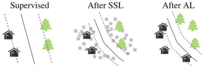
Supervised After SSL After AL

Fig. 1. Regularization of models with unlabeled samples: (left) purely supervised solution, (middle) semisupervised so-lution exploiting low density areas, and (right) active learning solution, where three new samples are labeled by a user.

Table 1. Summary of semisupervised algorithms used in HSI classification.

Assumption Model Idea

Low-density TSVM [11] Look for the emptiest margin Manifold Label

propaga-tion [12]

Spread class information on the graph of labeled/unlabeled (nearby samples are classified in the same class) Laplacian

SVM [14]

SVM hinge loss plus Laplacian eigen-maps for manifold regularization: Pix-els close in the input space are also close in the graph (nearby samples are mapped close together)

SSNN [7] Neural network trained with gradient descent replaces SVM, graph regular-ization with loss that forces similar pix-els to be mapped closely and dissimilar ones to be separated

Cluster Cluster ker-nel [13]

Increase the similarity measure (kernel) if samples fall in the same cluster, then run standard SVM

Mean map kernel [15]

Increase similarity if samples are mapped close to centroids in Hilbert space, then run standard SVM

representing the various land cover types of the environment. Many different marsh subclasses were merged in a ‘marsh’ class, resulting into the following10 classes: ‘Water’ (761

labeled pixels), ‘Mud flats’ (243), ‘Marsh’ (898), ‘Hardwood swamp’ (105), ‘Dark/broadleaf’ (431), ‘Slash pine’ (520),

‘CP/Oak’ (404), ‘CP Hammock’ (419), ‘Willow’ (503), and

‘Scrub’ (927). The high dimensionality and number of classes

and subclasses pose challenging problems for the classifiers, especially when few labeled examples are available.

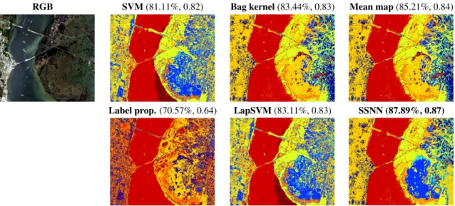
Figure 2 illustrates classification results for cluster ker-nels, probabilistic mean map kernel, label propagation, Lapla-cian SVM (LapSVM), and semisupervised neural networks (SSNN). We used` = 200labeled pixels (20per class) and

u = 1000 unlabeled pixels. LapSVM, cluster kernels and mean map kernels perform similarly, and all improve the re-sults of the label propagation whose training was particularly difficult in this high dimensional setting. More homoge-neous areas and better classification maps are observed in general for the mean map and bag kernels, and particularly for the SSNN, which efficiently deals with complex marsh areas (south east area of the image) and cope with large scale datasets.

Regularization via user’s interaction. Another possibility to cope with small sample problems is to provide additional la-beled examples. This is possible since HSI represent land sur-faces, usually physically reachable or that can be displayed in an image processing software. Therefore, the new sam-ples can be collected either by photointepretation of the

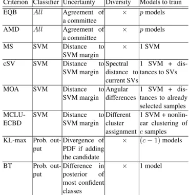
im-Table 2. Summary of active learning algorithms [16] (c:

num-ber of candidates,p: members of a committee of learners).

Criterion Classifier Uncertainty Diversity Models to train

EQB All Agreement of

a committee ⇥

pmodels

AMD All Agreement of

a committee ⇥ pmodels MS SVM Distance to SVM margin ⇥ 1 SVM cSV SVM Distance to

SVM margin Spectraldistance to current SVs

1 SVM + dis-tances to SVs

MOA SVM Distance to

SVM margin Angulardifferences 1 SVM + dis-tances to already selected samples

MCLU-ECBD SVM DistanceSVM margintoDifferentcluster assignment

1 SVM + nonlin-ear clustering of csamples KL-max Prob.

out-put Divergence of PDF if adding the candidate ⇥ (c 1)models BT Prob. out-put Difference in posterior of most confident classes ⇥ 1 model

ages (only if the classes can be recognized on screen) or by organizing field campaigns. However, since providing addi-tional samples is costly, the samples to be labeled must be selected carefully. To this end,active learning(AL [16, 17], right panel of Fig. 1) has gained popularity in the last years: rather than proceeding by random sampling or stratification (i.e. sampling according to a measure of the expected vari-ability within a class), AL uses the outcome of the current model to rank the unlabeled pixels according to their expected importance for future labeling. The aim is to detect the most difficult (and diverse) pixels for the current classifier. The top ranked pixels are then screened by a human operator, who provides the labels, enlarging the training set. With the en-larged training set, a new improved classifier is built and the process is iterated. Since AL focuses on difficult areas, it boosts the performances with fewer samples than those re-quired by random sampling. Figure 6 illustrates an example of active learning model regularization for the specific task of adapting classifiers to multiple scenes.

Regularization through sparsity promotion. Despite their high dimensionality, hyperspectral pixels belonging to the same class typically lie in a low-dimensional subspace. This observation was exploited in local semisupervised classifiers, and has been recently used in sparse signal representations. Here, the assumption is that pixels can be represented accu-rately as a linear combination of a few training samples from a structured dictionary.

RGB SVM(81.11%, 0.82) Bag kernel(83.44%, 0.83) Mean map(85.21%, 0.84)

Label prop.(70.57%, 0.64) LapSVM(83.11%, 0.83) SSNN (87.89%, 0.87)

Fig. 2. RGB composition and classification maps with SVM, bag kernels, probabilistic mean map kernel, label propagation, LapSVM, and SSNN for the KSC image (`= 200,u= 1000). Overall accuracy and kappa statistic are given in brackets.

Note the connection with SVMs that embed the dictio-nary (the training samples) into a high dimensional feature space_H. The use of the hinge loss in the SVM functional induces a sparse solution, i.e. few training examples are se-lected. Recently, sparse kernel methods have been presented, such as the kernel matching pursuit, the`1-SVM, the kernel

basis pursuit or the generalized LASSO. In all these, the dic-tionary functions are the kernels centered around the selected ‘support vectors’. Alternatively, in [18], several sparse kernel approaches have been presented with a different philosophy: the target pixel is the test pixel itself, not a similarity evalu-ation, and the dictionary is composed by the training pixels in the feature space. In this paper, a Basis Projection (BP) approach is used to promote sparsity with⌦=_kw_k1, as a

re-laxation of the more computationally demanding problem in-duced by using the`0-norm. To solve the BP problem, greedy

algorithms, such as the orthogonal matching pursuit (OMP) and the subspace pursuit (SP) methods, can be used. The dictionary can be obtained off-line or from the same image. The classification can be additionally improved by incorpo-rating the contextual information from the neighboring pixels into the classifier (see the next Section).

In the example illustrated in Fig. 3, we compare the per-formance of the linear (SP, OMP) and kernel (KSP, KOMP) sparse HSI classifiers introduced in [18]. The sparseness fac-tor was tuned for best performance. We also included a linear SVM and the⌫-SVM using an RBF kernel, in which the

pa-rameter⌫ ₂(0,1)controls the degree of sparsity. The RBF

parameter was tuned by standard10-fold cross-validation.

Figure 3 shows the results for these methods and different number of training samples in the standard AVIRIS Indian Pines hyperspectral image (220spectral channels and spatial

resolution20m, shown in Fig. 5). This is the standard

bench-mark hyperspectral image which is used here to allow

com-0 5 10 15 20 25 30 0.55 0.6 0.65 0.7 0.75 0.8 0.85 0.9

Rate of training samples, [%]

Kappa statistic, κ SP KSP OMP KOMP linear SVM ν−SVM

Fig. 3. Performance measure with the estimated Cohen’s kappa statistic,, for different sparsity-promoting classifiers. parison with results in [18]. We split the data into a training set (20% of the available labeled pixels) and a test set (80%). We trained the classifiers for different rates{1, 5, 10, 15, 20, 25, 30}% of the training set, and show results for the test set that remained constant. Nonlinear methods show a much bet-ter performance over linear approaches. In the linear case, SP clearly outperforms the rest, but when the nonlinearity is included all methods perform very similarly.

SPATIAL-SPECTRAL IMAGE CLASSIFICATION

Hyperspectral images live in ageographical manifold, in the sense that spatially neighboring pixels carry correlated in-formation and that images are usually smooth in the spatial domain [1][see Ch. 2]. Accounting for spatial smoothness (i) provides less salt-and-pepper classification maps, (ii) re-veals the size and shape of the structure the pixel belongs to, and (iii) allows to discriminate between structures made of

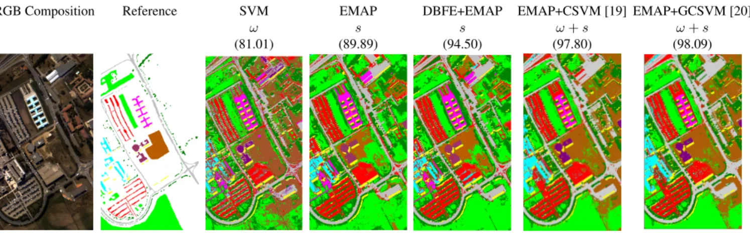
RGB Composition Reference SVM EMAP DBFE+EMAP EMAP+CSVM [19] EMAP+GCSVM [20]

! s s !+s !+s

(81.01) (89.89) (94.50) (97.80) (98.09)

Fig. 4. RGB composition along with the available reference data for the ROSIS-03 Pavia University area data set (103 spectral channels and spatial resolution 1.3m). Classification maps are shown for SVM on the original image only against spatio-spectral classification with the EMP, EMAP and EMAP after feature extraction by DBFE (81 data channels), composite kernels wth cross-kernels and SVM [19], and generalized composite kernels with multinomial logistic regression [20]. Overall accuracies [%] are reported in parentheses (!: using spectral bands,s: using spatial filters from PCA).

the same materials, but belonging to different land-use types. Spatial regularization has been widely used to improve classi-fication [21]. The joint exploitation of bothspectraland spa-tialinformation considers that either the loss, the regularizer, or both depend on the spatial neighbourhood of a pixel [22]. Spatial feature extraction. A simple yet effective way to reg-ularize for spatial smoothness is to enrich the input space with features accounting for the neighborhood of the pixels. This is usually done by using moving windows or adaptive filters applied to the spectral bands. These filtered images are then used to learn the classifier. Standard filters based on occur-rence or co-occuroccur-rence, morphological operators, Gabor fil-ters or wavelets decompositions generally provide significant improvements over purely spectral classifiers. Among them, morphological filters are the most promising. In [23], filtering was performed at many scales and anExtended Morpholog-ical Profile (EMP) was used for classification. Proceeding in a multiscale fashion enables the adaptive definition of the neighborhood of a pixel according to the structure it belongs to. Filtering in HSI is more challenging than in multispectral images, and one typically resorts to compute the EMP based on only a few Principal Components (PCs) using morpholog-ical reconstruction operators. All the features are then fed to a classifier, either alone [23] or combined with the original spectral information [24]. Furthermore, feature selection [25] or extraction [23] can be used to find the relevant features. Recently, connected tree-based morphological operators have been investigated for the analysis of HSI [26]. These so-called attribute filters extract thematic attributes of the connected components of an image which are thresholded according to their geometry (area, length, shape factors), or texture (range, entropy). The multiscale version, Extended Morphological Attribute Profile (EMAP), has been also introduced.

In Fig. 4, the approaches based on mathematical morphol-ogy (EMP and EMAP extracted from the first four princi-pal components) are used for classification of ROSIS-03 data from an urban area in Pavia, Italy. We selected this image to illustrate the capabilities of several spatial-spectral classifiers since urban areas monitoring at VHR typically requires the extraction of directional, rotational and scale features from objects. A significant improvement in terms of classification accuracies with respect to the spectral SVM was achieved by applying the EMAP with four different attributes on the image (area and diagonal of the bounding box of connected compo-nents, moment of inertia and standard deviation, see [26]). On the other hand, some redundancy was observed in the original 144–dimensional filter vector of EMAP. Therefore, Decision Boundary Feature Extraction (DBFE) was applied on it. After extraction with DBFE, the accuracies improved significantly (+5%), thus confirming the importance of feature extraction routines. Finally, comparison with composite kernels (see discussion below in Sect. [19, 20]) yielded improved classi-fication accuracy, but with a strong change of response in the right part of the image, where much more soil is predicted. This is explained by the fact that these two approaches jointly use spectral and spatial information, and are thus closer to the original spectral SVM result (for which the right part was partially predicted as soil).

Spatial-spectral segmentation. Another approach for the in-clusion of spatial information is through imagesegmentation, typically using watershed, mean shift and hierarchical seg-mentation [21]. After segseg-mentation, a supervised scheme assigns the pixels in the segments to the classes. Two ap-proaches are the mostly used: in the first, the regions are treated as input vectors in a supervised classifier. In the sec-ond regions are considered as basins to post-process the class

RGB SVM (78.2%, 0.75)

Majority Voting (90.8%, 0.90) Markers (91.8%, 0.91)

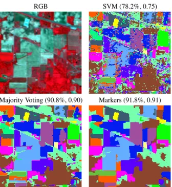
Fig. 5. RGB composition of the standard AVIRIS Indian Pine data set (200 spectral channels and spatial resolution 20m). Classification maps are shown for spatio-spectral clas-sificaiton with the segmentation and classification with major-ity voting and segmentation with markers against SVM on the original image only. Overall accuracies and the kappa statistic for each method are reported in parentheses [21].

memberships attributed by a pixel-based classifier within each segment.

The reverse view on the problem is proposed in [27], where a supervised classifier is used to produce confidence values for each pixel. Then, pixels with maximal confidence are used as seeds for a region growing algorithm. In [28] segmentation and classification are linked by user-provided labels: working with a hierarchical segmentation of the data, the labels provided are used to isolate coherent clusters, both spatially and thematically, thus ending with the good segmen-tation and the labels of the segments. The number of queries is minimized with active learning.

In Fig. 5, two approaches based on segmentation and classification with majority voting and markers are applied to a 220-bands AVIRIS dataset over Indian Pines (Indiana, USA). Significant improvement in terms of overall classifi-cation accuracies and kappa statistic were achieved over the pixel-based SVM classifier. Using markers provided the best accuracies: a +1%improvement over the simple majority

voting and more than+13%over the traditional pixel-based

SVM classifier. Furthermore, as seen in Fig. 5, it is clear that the classification and segmentation approaches provide a sig-nificantly more uniform classification map when compared to the purely spectral SVM classification map.

Table 3. Summary of spatial-spectral algorithms Type ofAAA

Approach Model Idea

Spatial filters extraction

Co-occurrence Extract texture based on statis-tics of pairs of pixels in a neighborhood

EMP Multiscale mathematical mor-phology (based on size) EMAP Multiscale mathematical

mor-phology (variety of attribute types) Spatial-spectral segmentation Segmentation and classification based on majority voting

All pixels are assigned to the most frequent class inside a segmented region

Segmentation and classification based on markers

Most reliably classified pixels are selected as “region mark-ers” for segmentation Semi-supervised

hierarchical clus-tering tree

Returns both classification and confidence maps. Active learning used to select infor-mative samples. Advanced spatial-spectral Composite and multiple kernels

Balances between spatial and spectral information with ded-icated kernels

classification Graph kernels Takes into account higher or-der relations in each pixel neighborhood

MRF Markov Random Field Model-ing (probabilistic)

Advanced spatial-spectral classifiers. The main problem with spatial-spectral feature extraction approaches is the possibly high-dimensionality of the feature vectors to feed the clas-sifier. This was alleviated in [19] where dedicated kernels for the spectral and spatial information were combined. The framework has been recently extended to deal with convex combinations of kernels through multiple-kernel learning [25] and generalized composite kernels [20]. In both cases, how-ever, the methodology still relies on performing anad hoc spatial feature extraction before kernel computation. Other alternatives in the literature considered the definition of graph kernels that capture multiscale higher-order relations in a neighborhood without computing them explicitly [29], and the modification of the SVM to seek for the spatial filter that maximizes the margin [30].

A final alternative is to include contextual information with Markov Random Fields (MRF), which naturally include a spatial term on class smoothness in the energy function. However, in the high dimensional context of HSI, the standard application of the neighbor system definition makes the prob-lem computationally intractable, and therefore recent works have focused on joining MRF spatial priors and discrimina-tive models in HSI classification [31,32]. An excellent review of MRF spatial-spectral methods can be found in [33].

ADAPTATION AND INVARIANCES

One of the greatest challenges of modern HSI classification is the adaptation of classifiers between acquisitions that differ either by the zone they represent and/or the acquisition con-ditions such as illumination, angle and season, among other effects. Adaptation is a central issue in HSI classification. For example, the increase in revisit time of recent satellites has improved multitemporal analysis of scenes. Nevertheless, al-gorithms must be able to adapt to changing situations. Gener-ally, the direct application of classifiers trained on one image to new images leads to poor results: even if the objects rep-resented in the images are roughly the same, differences in acquisition induce significantlocalchanges in the probability distribution function (PDF). These changes must be modeled and introduced in the classifiers. The concept ofadaptation can be implemented at the levels of image pre-processing, ro-bust and invariant feature extraction, or in the design of the classification algorithm.

Preprocessing. The pre-processing phase can address adap-tation through the use of radiometric correction techniques applied to the images. Absolute corrections aim at trans-forming the radiance measured at the sensor into surface re-flectance.Relative calibrationtechniques adapt the radiomet-ric properties between portions of an image or between im-ages. Generally, absolute correction techniques require addi-tional ground reference data that in many cases are not avail-able or are difficult to collect. Relative calibration methods are often considered as a pragmatic alternative for adaptation. Among these methods, we recall histogram matching, relative radiometric normalization of time series [34], and multivari-ate histogram matching [35].

Images can be casted as point clouds in a geometrical space endorsed with an appropriate distance measure. Such a view is quite convenient because it allows us to move from image adaptationtomanifold adaptation. Recent methods have explicitly considered the distortions occurring between image manifolds. In [36], multitemporal sequences for each pixel were aligned based on a measure of similarity between sequences barycenters, thus consisting into a global measure of alignment. In [37], spectra of the pixels are spatially de-trended using Gaussian processes in order to avoid shifts re-lated to geometrical differences or to localized class variabil-ity. A recent principled approach tries to match graphs rep-resenting the data manifolds [38]. There, the graphs of the two domains are matched using a procedure aiming at maxi-mizing their similarity, while at the same time preserving the original structure of the graphs.

Adapting the classifier. Learning a transformation between domains may be insufficient to handle all the perturbing fac-tors, so alternative approaches are concerned with the adap-tation of the classifier itself. From a machine learning

per-150 250 350 450 550 0.65 0.7 0.75 0.8 0.85 0.9 # of labeled pixels Ka p p a 150 from S + 400 random pixels on T 550 from T 150 pixels from S only

150 from S + 400 selected with active learning on T

S only T only S + T random S + T active T T(reference) S S (reference)

Fig. 6. Use of active learning to adapt a maximum likelihood classifier [40]. Left: given an image and a set of reference pixels in a first source area (S), we want to classify another spatially disconnected target area (T), by adding labels cho-sen actively in the reference ofT. Center: learning curves for the active (solid red line) and random sampling (dashed green line), evolving between the extremes of a model with-out adaptation (black dot at 150 samples), and another ac-tively adapted that uses 550 samples randomly selected from

T (blue dashed line). Right: classification maps in the target

domain_T. The color of the bounding box in each map refers to the legend in the central plot.

spective, the problem of classifier adaptation is studied in the framework of transfer learning, and in particular of domain adaptation. Domain adaptation reduces to learning from data in a source domain_S(e.g. a portion of an image) to extrap-olate to a different target domain_T (another portion of the image or to another image). The problem has been payed at-tention in HSI classification lately [39]. In this setting, source and target domains are assumed to share the same set of infor-mation classes (exceptions to this constraint in [40,41]) and to follow similar (but not the same) class distributions. Domain adaptation problems in remote sensing have been mainly ad-dressed with semisupervised techniques, which exploit the la-beled samples fromSand the unlabeled samples fromT in order to derive a classification rule suitable for the target do-main. The most recent developments in this sense consider semisupervised and domain adaptation SVMs [39], Gaussian processes [37, 41] and the mean-map kernel methods [15].

Recently, active learning has been also used for adapta-tion assuming that some samples (as few as possible) from the target domain can be labeled by the user and added to the existing training set (defined on_S) in order to adapt the clas-sifier to the target domain_S[40, 42]. This makes the adapta-tion process more robust than in the case of semi-supervised learning at the cost of requiring additional labeled samples. Figure 6 illustrates this principle for a102-bands image of the

city center of Pavia acquired by the ROSIS-03 airborne sen-sor. The whole image (only a portion is shown) has a size of

1400⇥512pixels and spatial resolution is1.3m. Five classes

of interest (buildings, roads, water, vegetation and shadows) are considered, and a total of206,009labeled pixels are

avail-able. We explore the potential of migrating a classifier built on a source areaSwith as few labeled pixels as possible from the rest of the imageT. First, the model trained with 150

labeled pixels randomly drawn fromS was directly applied toT and yielded a_S of0.67. Noticeably, a classifier built on550samples randomly selected onT reached_S = 0.84. This suggests that different regions of the same scene follow very different statistics for classification. In order to improve the first classifier, we enlarged the first training set with la-beled samples drawn from T, either taken through random sampling (RS, green dashed line) or with active learning (AL, red solid line). Using AL allows to concentrate efforts in ar-eas where the first model is suboptimal, so performance is im-proved with respect to RS. After400queries (thus, a model

using550training samples in total), random sampling yields

similar performance to a model using 550randomly drawn

pixels (RS = 0.84), while active learning improves the re-sults withAL= 0.89. To reach the performance of the model using 550 random pixels, AL requires only 120 active queries (thus a total of 270 samples in the model).

Extracting and encoding invariances in the classifier. Image classifiers must be robust to changes in the data representa-tion within each land cover class. The property of such math-ematical functions is called ‘invariance’. A classifier should be invariant to object rotations, to changes in illumination, to the presence of shadows, and to the spatial scale of the objects to be detected. Extracting robust features (invariants) for classification and domain adaptation has been traditionally pursued by looking at the spatial or the spectral signal char-acteristics. On the one hand,scale invariants aim to make classifiers invariant to perturbations of object scales. In HSI classification, a single spatial scale is typically suboptimal be-cause different classes exhibit diverse sizes, shapes, and inter-nal variations. Multiscale classification schemes may allevi-ate these problems. Also, following wavelet-based represen-tations and exploiting SIFT descriptors,translation invariants have been recently explored. On the other hand,spectral in-variantsare considered the fundamental descriptors of object structure, and are commonly employed to characterize canopy structure. Spectral invariance to daylight illumination allows for example improving multitemporal image classification.

Incorporating invariances in SVM can be achieved by de-signing particular kernel functions that encode local invari-ance under transformations, or to generate artificial examples for training to which the model must be invariant. In the fol-lowing example, we consider the latter possibility, with the Virtual SVM (VSVM) method, which has been successfully exploited to encode scale, rotation, translation and shadow in-variance in HSI classification [43].

In Fig. 7, we illustrate the use of the VSVM encoding (spectral) shadow-invariance for image classification. We use the same data acquired by the ROSIS-03 optical sensor of the city center of Pavia (Italy) used in Fig. 6. We perform

RGB SVM (0.79±0.11) VSVM (0.84±0.09)

Fig. 7. Experiment of patch-based classification with the vir-tual SVM encoding shadow invariance. True-color composite (left), and classification maps using the standard SVM (mid-dle) and the VSVM (right) obtained using50training pixels.

Results are shown in parentheses in the form of (mean± stan-dard deviation ofin 20 realizations).

patch-based classification using only50 training patches of

size w = 5. The classes to be detected are, as for Fig. 6,

buildings, roads, water, vegetation and shadows. Virtual sup-port vectors (VSVs) were generated according to the observed exponential behavior of the ratio shadow/sunlit as a function of the wavelength [43]. Numerical results, as well as the zoom on a detail of the classification map, show that VSVM leads to more accurate results than the standard SVM: en-coding shadow invariance reduces misclassifications on the bridge area and an overall more homogeneous classification over flat areas (see for example the crossroads in the center of the image).

CONCLUSIONS AND DISCUSSION

This paper reviewed and analyzed the recent developments in hyperspectral image classification. Even though HSI follow similar spatial, spectral and spatial-spectral image statistics to those conveyed by conventional photographic images, the hyperspectral signals impose additional challenges related to their high dimensionality and heterogeneity. Therefore, even though standard techniques in image processing and com-puter vision may be transported drectly, HSI impose impor-tant constraints to develop efficient and effective classifiers.

The use of methods derived from statistical learning the-ory (SLT) has been a driving factor in recent years. SLT con-stitutes a proper framework to tackle the problems posed by hyperspectral remote sensing images, which typically involve scenarios with high dimensional data and few training sam-ples. SLT permit to embed numerical regularization in non-linear classifiers, and also to design alternative forms of con-ditioning and incorporation of prior knowledge. Additionally, classification is often improved by including spatially-based and manifold-based regularizers. SLT also allows to design

sparse methods able to work in relevant feature subspaces, where compact and computationally efficient method can be run. Finally, the SLT framework has allowed to include prior knowledge in a very fruitful way: for example, classifiers can now incorporate spatial and spectral invariances that disen-tangle ambiguities present in land cover classification.

The field is moving fast, and attracts research from the computer vision and machine learning communities. New ap-proaches are introduced regularly and permit to tackle new scenarios issued from high resolution imaging (e.g. multi-temporal, multiangular), while learning the relevant features via robust classifiers. It should be also noted that, with up-coming satellites, efficient algorithms for dimensionality re-duction before classification and fast/parallel computing so-lutions will be necessary to accelerate the interpretation and efficient exploitation of hyperspectral images.

ACKNOWLEDGMENTS

This work was partially supported by the Spanish Ministry of Economy and Competitiveness (MINECO) under project LIFE-VISION TIN2012-38102-C03-01, and by the Swiss National Research Foundation under grant PZ00P2-136827. AUTHORS

Gustavo Camps-Valls ([email protected]) (SM’07) re-ceived a Ph.D. degree in Physics (2002) from the Universitat de Val`encia, Spain, where he is currently an Associate Profes-sor in the Electrical Engineering Dept. and head of the Image and Signal Processing group. His research is tied to machine learning for signal and image processing, with special focus on remote sensing data analysis. He has co-authored many journal papers and edited several books on kernel methods. The ISI lists him as a highly cited researcher. He is member of the Machine Learning for Signal Processing TC of the IEEE SPS, and serves as Associate Editor for IEEE Transac-tions on Signal Processing, IEEE Signal Processing Letters, and IEEE Geoscience and Remote Sensing Letters. Visit http://isp.uv.es/ for more information.

Devis Tuia([email protected]) received a Ph.D in environ-mental sciences at the Univeristy of Lausanne (Switzerland) in 2009. He was then a postdoc researcher at both the Uni-versity of Val`encia, Spain and the UniUni-versity of Colorado at Boulder. He is now senior research associate at the laboratory of Geographic Information Systems, at the Ecole Polytech-nique F´ed´erale de Lausanne (EPFL). His research interests include the development of algorithms for information ex-traction and classification of very high resolution remote sensing images using machine learning algorithms. Visit http://devis.tuia.googlepages.com/ for more information.

Lorenzo Bruzzone([email protected]) received the Ph.D. degree in Telecommunications Engineering from the University of Genoa, Italy, in 1998. He is currently a Full

Professor at the University of Trento, Italy where he is the founder and the head of the Remote Sensing Laboratory. His current research interests are in the areas of remote sensing, radar and SAR, signal processing, and pattern recognition. He is the author (or coauthor) of many highly cited scientific publications in referred international journals, conference proceedings, and book chapters. He is the co-founder of the IEEE International Workshop on the Analysis of Multi-Temporal Remote-Sensing Images (MultiTemp) series. Since 2003 he has been the Chair of the SPIE Conference on Im-age and Signal Processing for Remote Sensing. Since 2013 he has been the founder Editor-in-Chief of the IEEE Geo-science and Remote Sensing Magazine. He is a member of the Administrative Committee of the IEEE Geoscience and Remote Sensing Society (GRSS) and a Distinguished Speaker of the IEEE GRSS. He is Fellow of IEEE. Visit http://rslab.disi.unitn.it for more information.

J´on Atli Benediktsson([email protected]) received the Ph.D. degree in electrical engineering from Purdue University, West Lafayette, IN in 1990. He is currently Pro Rector for Aca-demic Affairs and Professor of Electrical and Computer Engineering at the University of Iceland. His research in-terests are in remote sensing, biomedical analysis of signals, pattern recognition, image processing, and signal processing. He was a co-founder of Oxymap, Inc. Prof. Benediktsson was the 2011-2012 President of the IEEE Geoscience and and Remote Sensing Society. He was Editor-in-Chief of the IEEE Transactions on Geoscience and Remote Sensing (2003-2008). He is a Fellow of IEEE and a Fellow of SPIE. Visit www.hi.is/⇠benedikt for more information.

REFERENCES

[1] G. Camps-Valls, D. Tuia, L. G´omez-Chova, S. Jimenez, and J. Malo,

Remote Sensing Image Processing, Synthesis Lectures on Image, Video, and Multimedia Processing. Morgan and Claypool, 2011. [2] G. Camps-Valls and L. Bruzzone, “Kernel-based methods for

hyper-spectral image classification,”IEEE Trans. Geosci. Remote Sens., vol.

43, no. 6, pp. 1351–1362, 2005.

[3] V. Vapnik,Statistical Learning Theory, Wiley, NJ, USA, 1998.

[4] T. V. Bandos, L. Bruzzone, and G. Camps-Valls, “Classification of

hy-perspectral images with regularized linear discriminant analysis,”IEEE

Trans. Geosci. Remote Sens., vol. 47, no. 3, pp. 862–873, 2009. [5] A. C. Jensen, M. Loog, and A. H. Schistad Solberg, “Using

multi-scale spectra in regularizing covariance matrices for hyperspectral

im-age classification,” IEEE Trans. Geosci. Remote Sens., vol. 48, no. 4,

pp. 1851–1859, 2010.

[6] Jun Li, J.M. Bioucas-Dias, and A. Plaza, “Spectral-spatial hyperspec-tral image segmentation using subspace multinomial logistic regression

and Markov random fields,”IEEE Trans. Geosci. Remote Sens., vol. 50,

no. 3, pp. 809–823, 2012.

[7] F. Ratle, G. Camps-Valls, and J. Weston, “Semisupervised neural

net-works for efficient hyperspectral image classification,” IEEE Trans.

Geosci. Rem. Sens., vol. 48, no. 5, pp. 2271–2282, 2010.

[8] F.A. Mianji and Ye Zhang, “Robust hyperspectral classification using

relevance vector machine,”IEEE Trans. Geosci. Remote Sens., vol. 49,

[9] Y. Bazi and F. Melgani, “Gaussian process approach to remote sensing

image classification,” IEEE Trans. Geosci. Remote Sens., vol. 48, no.

1, pp. 186–197, 2010.

[10] G. Camps-Valls and L. Bruzzone,Kernel Methods for Remote Sensing

Data Analysis, J. Wiley & Sons, NJ, USA, 2009.

[11] L. Bruzzone, M. Chi, and M. Marconcini, “A novel transductive SVM

for semisupervised classification of remote sensing images,” IEEE

Trans. Geosci. Remote Sens., vol. 44, no. 11, pp. 3363–3373, 2006. [12] G. Camps-Valls, T. Bandos, and D. Zhou, “Semisupervised

graph-based hyperspectral image classification,” IEEE Trans. Geosci. Rem.

Sens., vol. 45, no. 10, pp. 3044–3054, 2007.

[13] D. Tuia and G. Camps-Valls, “Semi-supervised remote sensing image

classification with cluster kernels,” IEEE Geosci. Remote Sens. Lett.,

vol. 6, no. 1, pp. 224–228, 2009.

[14] L. G´omez-Chova, G. Camps-Valls, J. Mu˜noz-Mar´ı, and J. Calpe, “Semi-supervised image classification with Laplacian support vector

machines,” IEEE Geosci. Remote Sens. Lett., vol. 5, no. 4, pp. 336–

340, 2008.

[15] L. G´omez-Chova, G. Camps-Valls, L. Lorenzo Bruzzone, and J. Calpe-Maravilla, “Mean map kernels for semi-supervised cloud

classifica-tion,” IEEE Trans. Geosci. Remote Sens., vol. 48, no. 1, pp. 207–220,

2010.

[16] D. Tuia, M. Volpi, L. Copa, M. Kanevski, and J. Mu˜noz-Mar´ı, “A sur-vey of active learning algorithms for supervised remote sensing image

classification,”IEEE J. Sel. Topics Signal Proc., vol. 5, no. 3, pp. 606–

617, 2011.

[17] M. M. Crawford, D. Tuia, and L. H. Hyang, “Active learning: Any

value for classification of remotely sensed data?,” Proc. IEEE, vol.

101, no. 3, pp. 593–608, 2013.

[18] Yi Chen, N.M. Nasrabadi, and T.D. Tran, “Hyperspectral image

clas-sification via kernel sparse representation,”IEEE Trans. Geosci. Rem.

Sens., vol. 51, no. 1, pp. 217–231, 2013.

[19] G. Camps-Valls, L. G´omez-Chova, J. Mu˜noz-Mar´ı, J. Vila-Franc´es, and J. Calpe-Maravilla, “Composite kernels for hyperspectral image

clas-sification,” IEEE Geosci. Remote Sens. Lett., vol. 3, no. 1, pp. 93–97,

2006.

[20] J. Li, P. R. Marpu, A. Plaza, J. Bioucas-Dias, and J. A. Benedikts-son, “Generalized composite kernel framework for hyperspectral image

classification,”IEEE Trans. Geosci. Remote Sens., in press.

[21] M. Fauvel, Y. Tarabalka, J. A. Benediktsson, J. Chanussot, and J. C. Tilton, “Advances in spectral-spatial classification of hyperspectral

im-ages,”Proc. IEEE, vol. 101, no. 3, pp. 652 – 675, 2013.

[22] A. Plaza, J. A. Benediktsson, J. Boardman, J. Brazile, L. Bruzzone, G. Camps-Valls, J. Chanussot, M. Fauvel, P. Gamba, A. Gualtieri, M. Marconcini, J.C. Tilton, and G. Trianni, “Recent advances in

tech-niques for hyperspectral image processing,” Remote Sens. Environ.,

vol. 113, no. Supplement 1, pp. S110–S122, 2009.

[23] J. A. Benediktsson, J. A. Palmason, and J. R. Sveinsson, “Classification of hyperspectral data from urban areas based on extended

morpholog-ical profiles,” IEEE Trans. Geosci. Remote Sens., vol. 43, no. 3, pp.

480–490, 2005.

[24] M. Fauvel, J. A. Benediktsson, J. Chanussot, and J. R. Sveinsson, “Spectral and spatial classification of hyperspectral data using SVMs

and morphological profiles,” IEEE Trans. Geosci. Remote Sens., vol.

46, no. 11, pp. 3804 – 3814, 2008.

[25] D. Tuia, G. Camps-Valls, G. Matasci, and M. Kanevski, “Learning

rel-evant image features with multiple kernel classification,” IEEE Trans.

Geosci. Remote Sens., vol. 48, no. 10, pp. 3780 – 3791, 2010. [26] M. Dalla Mura, J. A. Benediktsson, B. Waske, and L.; Bruzzone,

“Mor-phological attribute profiles for the analysis of very high resolution

im-ages,” IEEE Trans. Geosci. Remote Sens., vol. 48, no. 10, pp. 3747–

3762, 2010.

[27] Y. Tarabalka, J. Chanussot, and J. A. Benediktsson, “Segmentation and classification of hyperspectral images using minimum spanning forest

grown from automatically selected markers,” IEEE Trans. Sys. Man

Cybernetics B, vol. 40, no. 5, pp. 1267 –1279, 2010.

[28] J. Mu˜noz-Mar´ı, D. Tuia, and G. Camps-Valls, “Semisupervised

clas-sification of remote sensing images with active queries,” IEEE Trans.

Geosci. Remote Sens., vol. 50, no. 10, pp. 3751–3763, 2012.

[29] G. Camps-Valls, N. Shervashidze, and K.M. Borgwardt,

“Spatio-spectral remote sensing image classification with graph kernels,”IEEE

Geosci. Remote Sens. Lett., vol. 7, no. 4, pp. 741–745, 2010. [30] R. Flamary, D. Tuia, B. Labbe, G. Camps-Valls, and A.

Rakotoma-monjy, “Large margin filtering,”IEEE Trans. Signal Proc., vol. 60, no.

2, pp. 648–659, 2012.

[31] Y. Tarabalka, M. Fauvel, J. Chanussot, and J. A. Benediktsson, “SVM-and MRF-based method for accurate classification of hyperspectral

im-ages,” IEEE Geosci. Remote Sens. Lett., vol. 7, no. 4, pp. 736 –740,

2010.

[32] G. Moser and S. B. Serpico, “Combining support vector machines and Markov random fields in an integrated framework for contextual image

classification,” IEEE Trans. Geosci. Remote Sens., vol. 51, no. 5, pp.

2734–2752, 2013.

[33] G. Moser, S. B. Serpico, and J. A. Benediktsson, “Land-cover mapping

by Markov modeling of spatial-contextual information,” Proc. IEEE,

vol. 101, no. 3, pp. 631–651, 2013.

[34] M. J. Canty, A. A. Nielsen, and M. Schmidt, “Automatic radiometric

normalization of multitemporal satellite imagery,” Remote Sens.

Envi-ron., vol. 91, pp. 441–451, 2004.

[35] S. Inamdar, F. Bovolo, L. Bruzzone, and S. Chaudhuri, “Multidimen-sional probability density function matching for pre-processing of

mul-titemporal remote sensing images,”IEEE Trans. Geosci. Remote Sens.,

vol. 46, no. 4, pp. 1243–1252, 2008.

[36] F. Petitjean, J. Inglada, and P. Gancarski, “A global averaging method

for dynamic time warping, with applications to clustering,” Pattern

Recogn., vol. 44, no. 3, pp. 678–693, 2011.

[37] G. Jun and J. Ghosh, “Spatially adaptive classification of land cover

with remote sensing data,”IEEE Trans. Geosci. Remote Sens., vol. 49,

no. 7, pp. 2662–2673, 2011.

[38] D. Tuia, J. Mu˜noz-Mar´ı, L. G´omez-Chova, and J. Malo, “Graph

match-ing for adaptation in remote sensmatch-ing,” IEEE Trans. Geosci. Remote

Sens., vol. 51, no. 1, pp. 329–341, 2013.

[39] L. Bruzzone and M. Marconcini, “Domain adaptation problems: A DASVM classification technique and a circular validation strategy,”

IEEE Trans. Pattern Anal. Mach. Intell., vol. 32, no. 5, pp. 770–787, 2010.

[40] D. Tuia, E. Pasolli, and W. J. Emery, “Using active learning to adapt

remote sensing image classifiers,”Remote Sens. Environ., vol. 115, no.

9, pp. 2232–2242, 2011.

[41] G. Jun and J. Ghosh, “Semisupervised learning of hyperspectral data

with unknown land-cover classes,”IEEE Trans. Geosci. Remote Sens.,

vol. 51, no. 1, pp. 273–282, 2013.

[42] C. Persello and L. Bruzzone, “Active learning for domain adaptation in

the supervised classification of remote sensing images,” IEEE Trans.

Geosci. Remote Sens., vol. 50, no. 11, pp. 4468–4483, 2012.

[43] E. Izquierdo-Verdiguier, V. Laparra, L. G´omez-Chova, and G. Camps-Valls, “Encoding invariances in remote sensing image classification

with SVM,”IEEE Geosci. Remote Sens. Lett., vol. 10, no. 5, pp. 981–