Map overlay and
spatial aggregation in
sp
Edzer Pebesma
∗June 5, 2015
Abstract
Numerical “map overlay” combines spatial features from one map layer with the attribute (numerical) properties of another. This vignette ex-plains the R method “over”, which provides a consistent way to retrieve indices or attributes from a given spatial object (map layer) at the loca-tions of another. Using this, the R generic “aggregate” is extended for spatial data, so that any spatial properties can be used to define an aggre-gation predicate, and any R function can be used as aggreaggre-gation function.
Contents
1 Introduction 1
2 Geometry overlays 2
3 Using over to extract attributes 5
4 Lines, and Polygon-Polygon overlays require rgeos 7
5 Aggregation 10
1
Introduction
According to the free e-book by Davidson (2008),
An overlay is a clear sheet of plastic or semi-transparent paper. It is used to display supplemental map and tactical information related to military operations. It is often used as a supplement to orders given in the field. Information is plotted on the overlay at the same scale as on the map, aerial photograph, or other graphic being used.
∗Institute for Geoinformatics, University of Muenster, Weseler Strasse 253, 48151 M¨unster,
When the overlay is placed over the graphic, the details plotted on the overlay are shown in their true position.
This suggests that map overlay is concerned with combining two, or possibly
more, map layers by putting them on top of each other. This kind of overlay can be obtained in R e.g. by plotting one map layer, and plotting a second map layer on top of it. If the second one contains polygons, transparent colours can
be used to avoid hiding of the first layer. When using the spplot command,
thesp.layout argument can be used to combine multiple layers.
O’Sullivan and Unwin (2003) argue in chapter 10 (Putting maps together: map overlay) that map overlay has to do with the combination of two (or more) maps. They mainly focus on the combination of the selection criteria stemming from several map layers, e.g. finding the deciduous forest area that is less than
5 km from the nearest road. They call thisboolean overlays.
One could look at this problem as a polygon-polygon overlay, where we are looking for the intersection of the polygons with the deciduous forest with the polygons delineating the area less than 5 km from a road. Other possibilities are to represent one or both coverages as grid maps, and find the grid cells for which both criteria are valid (grid-grid overlay). A third possibility would be that one of the criteria is represented by a polygon, and the other by a grid (polygon-grid overlay, or grid-polygon overlay). In the end, as O’Sullivan and Unwin argue, we can overlay any spatial type (points, lines, polygons, pixels/grids) with any other. In addition, we can address spatial attributes (as the case of grid data), or only the geometry (as in the case of the polygon-polygon intersection).
This vignette will explain how theover method in packagespcan be used
to compute map overlays, meaning that instead of overlaying maps visually, the digital information that comes from combining two digital map layers is
retrieved. From there, methods to aggregate (compute summary statistics;
Heuvelink and Pebesma, 1999) over a spatial domain will be developed and demonstrated. Pebesma (2012) describes overlay and aggregation for spatio-temporal data.
2
Geometry overlays
We will use the wordgeometryto denote the purely spatial characteristics,
mean-ing that attributes (qualities, properties of somethmean-ing at a particular location)
are ignored. Withlocationwe denote a point, line, polygon or grid cell. Section
3 will discuss how to retrieve and possibly aggregate or summarize attributes
found there.
Given two geometries,AandB, the following equivalent commands
> A %over% B > over(A, B)
retrieve the geometry (location) indices of B at the locations of A. More in
locations inAnot matching with locations inB(e.g. those points outside a set of polygons).
Selecting points ofAinsideoronsome geometryB(e.g. a set of polygons)B
is done by > A[B,]
which is short for
> A[!is.na(over(A,B)),]
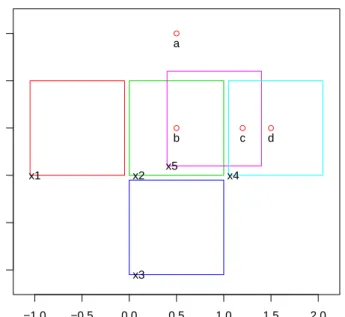
We will now illustrate this with toy data created by > library(sp) > x = c(0.5, 0.5, 1.2, 1.5) > y = c(1.5, 0.5, 0.5, 0.5) > xy = cbind(x,y) > dimnames(xy)[[1]] = c("a", "b", "c", "d") > pts = SpatialPoints(xy) > xpol = c(0,1,1,0,0) > ypol = c(0,0,1,1,0) > pol = SpatialPolygons(list( + Polygons(list(Polygon(cbind(xpol-1.05,ypol))), ID="x1"), + Polygons(list(Polygon(cbind(xpol,ypol))), ID="x2"), + Polygons(list(Polygon(cbind(xpol,ypol-1.05))), ID="x3"), + Polygons(list(Polygon(cbind(xpol+1.05,ypol))), ID="x4"), + Polygons(list(Polygon(cbind(xpol+.4, ypol+.1))), ID="x5")
+ ))
and shown in figure1.
Now, the polygonspolin which pointsptslie are
> over(pts, pol)
a b c d NA 5 5 4
As pointsbandcfall in two overlapping polygons, we can retrieve the complete
information as a list:
> over(pts, pol, returnList = TRUE)
$a
integer(0)
$b [1] 2 5
−1.0 −0.5 0.0 0.5 1.0 1.5 2.0 −1.0 −0.5 0.0 0.5 1.0 1.5 ● ● ● ● x1 x2 x3 x4 x5 a b c d
Figure 1: Toy data: points (a-d), and (overlapping) polygons (x1-x5)
[1] 4 5
$d [1] 4
and the appropriate points falling in any of the polygons are selected by > pts[pol] SpatialPoints: x y b 0.5 0.5 c 1.2 0.5 d 1.5 0.5
Coordinate Reference System (CRS) arguments: NA
The reverse, identical sequence of commands for selecting polygons pol that
have (one or more) points ofptsin them is done by
x1 x2 x3 x4 x5 NA 2 NA 3 2
> over(pol, pts, returnList = TRUE)
$x1 integer(0) $x2 [1] 2 $x3 integer(0) $x4 [1] 3 4 $x5 [1] 2 3 > row.names(pol[pts]) [1] "x2" "x4" "x5"
3
Using
over
to extract attributes
This section shows howover(x,y) is used to extract attribute values of
argu-mentyat locations ofx. The return value is either an (aggregated) data frame,
or a list.
We now create an exampleSpatialPointsDataFrame and a
SpatialPoly-gonsDataFrameusing the toy data created earlier:
> zdf = data.frame(z1 = 1:4, z2=4:1, f = c("a", "a", "b", "b"), + row.names = c("a", "b", "c", "d")) > zdf z1 z2 f a 1 4 a b 2 3 a c 3 2 b d 4 1 b > ptsdf = SpatialPointsDataFrame(pts, zdf) > zpl = data.frame(z = c(10, 15, 25, 3, 0), zz=1:5, + f = c("z", "q", "r", "z", "q"), row.names = c("x1", "x2", "x3", "x4", "x5")) > zpl
z zz f x1 10 1 z x2 15 2 q x3 25 3 r x4 3 4 z x5 0 5 q > poldf = SpatialPolygonsDataFrame(pol, zpl) In the simplest example
> over(pts, poldf) z zz f a NA NA <NA> b 15 2 q c 3 4 z d 3 4 z
adata.frameis created with each row corresponding to the first element of the
poldfattributes at locations inpts.
As an alternative, we can pass a user-defined function to process the table (selecting those columns to which the function makes sense):
> over(pts, poldf[1:2], fn = mean)
z zz a NA NA b 7.5 3.5 c 1.5 4.5 d 3.0 4.0
To obtain the complete list of table entries at each point ofpts, we use the
returnListargument:
> over(pts, poldf, returnList = TRUE)
$a
[1] z zz f
<0 rows> (or 0-length row.names)
$b z zz f x2 15 2 q x5 0 5 q $c z zz f
x4 3 4 z x5 0 5 q
$d
z zz f x4 3 4 z
The same actions can be done when the arguments are reversed: > over(pol, ptsdf) z1 z2 f x1 NA NA <NA> x2 2 3 a x3 NA NA <NA> x4 3 2 b x5 2 3 a > over(pol, ptsdf[1:2], fn = mean) z1 z2 x1 NA NA x2 2.0 3.0 x3 NA NA x4 3.5 1.5 x5 2.5 2.5
4
Lines, and Polygon-Polygon overlays require
rgeos
Package sp provides many of the over methods, but not all. Package rgeos
can compute geometry intersections, i.e. for any set of (points, lines, polygons) to determine whether they have one ore more points in common. This means
that the over methods provided by package sp can be completed by rgeos
for any over methods where a SpatialLines object is involved (either as x
or y), or where x and y are both of class SpatialPolygons (table 1). For
this purpose, objects of classSpatialPixelsorSpatialGridare converted to
SpatialPolygons. A toy example combines polygons with lines, created by > l1 = Lines(Line(coordinates(pts)), "L1")
> l2 = Lines(Line(rbind(c(1,1.5), c(1.5,1.5))), "L2") > L = SpatialLines(list(l1,l2))
and shown in figure2.
The set ofoveroperations on the polygons, lines and points is shown below
y: Points y: Lines y: Polygons y: Pixels y: Grid
x: Points s r s s s
x: Lines r r r r:y r:y
x: Polygons s r r s:y s:y
x: Pixels s:x r:x s:x s:x s:x
x: Grid s:x r:x s:x s:x s:x
Table 1: over methods implemented for different x and y arguments. s:
provided by sp; r: provided by rgeos. s:x or s:y indicates that the x or y
argument is converted to grid cell center points; r:x or r:y indicate grids or pixels are converted to polygons.
> library(rgeos) > over(pol, pol)
x1 x2 x3 x4 x5 1 2 3 4 2
> over(pol, pol,returnList = TRUE)
$x1 x1 1 $x2 x2 x5 2 5 $x3 x3 3 $x4 x4 x5 4 5 $x5 x2 x4 x5 2 4 5 > over(pol, L) x1 x2 x3 x4 x5 NA 1 NA 1 1 > over(L, pol)
−1.0 −0.5 0.0 0.5 1.0 1.5 2.0 −1.0 −0.5 0.0 0.5 1.0 1.5 x1 x2 x3 x4 x5 L1 L2
Figure 2: Toy data: two lines and (overlapping) polygons (x1-x5)
L1 L2 2 NA
> over(L, pol, returnList = TRUE)
$L1 x2 x4 x5 2 4 5 $L2 named integer(0) > over(L, L) L1 L2 1 2 > over(pts, L) a b c d 1 1 1 1
> over(L, pts)
L1 L2 1 NA
Another example overlays a line with a grid, shown in figure3.
5
Aggregation
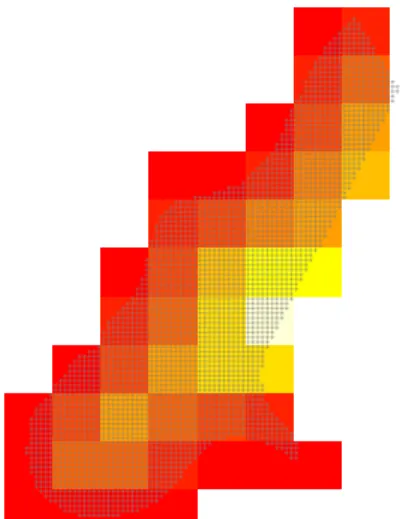
In the following example, the values of a fine grid with 40 m x 40 m cells are aggregated to a course grid with 400 m x 400 m cells.
> data(meuse.grid) > gridded(meuse.grid) = ~x+y > off = gridparameters(meuse.grid)$cellcentre.offset + 20 > gt = GridTopology(off, c(400,400), c(8,11)) > SG = SpatialGrid(gt) > agg = aggregate(meuse.grid[3], SG)
Figure 4 shows the result of this aggregation (agg, in colors) and the points
(+) of the original grid (meuse.grid). Function aggregateaggregates its first
argument over the geometries of the second argument, and returns a geometry
with attributes. The default aggregation function (mean) can be overridden.
An example of the aggregated values of meuse.grid along (or under) the
line shown in Figure??are
> sl.agg = aggregate(meuse.grid[,1:3], sl) > class(sl.agg) [1] "SpatialLinesDataFrame" attr(,"package") [1] "sp" > as.data.frame(sl.agg)
part.a part.b dist L1 0.4904459 0.5095541 0.3100566
Function aggregate returns a spatial object of the same class of sl (
Spa-tialLines), andas.data.frameshows the attribute table as adata.frame.
References
O’Sullivan, D., Unwin, D. (2003) Geographical Information Analysis.
Wi-ley, NJ.
Davidson, R., 2008. Reading topographic maps. Free e-book from: http:
> data(meuse.grid)
> gridded(meuse.grid) = ~x+y
> Pt = list(x = c(178274.9,181639.6), y = c(329760.4,333343.7)) > sl = SpatialLines(list(Lines(Line(cbind(Pt$x,Pt$y)), "L1"))) > image(meuse.grid)
> xo = over(sl, geometry(meuse.grid), returnList = TRUE) > image(meuse.grid[xo[[1]], ],col=grey(0.5),add=T) > lines(sl)
Figure 3: Overlay of line with grid, identifying cells crossed (or touched) by
Figure 4: aggregation over meuse.grid distance values to a 400 m x 400 m grid
Heuvelink, G.B.M., and E.J. Pebesma, 1999. Spatial aggregation and soil
process modelling. Geoderma 89, 1-2,47-65.
Pebesma, E., 2012. Spatio-temporal overlay and aggregation.
Pack-age vignette for packPack-age spacetime, http://cran.r-project.org/web/