Three Essays in Economics of Catastrophes
Edoardo Slerca
Faculty of Economics
Università della Svizzera italiana (USI)
Thesis submitted for the degree of
Doctor of Philosophy in Economics
Lugano, July 2018
Doctoral committee:
Prof. M. Jametti, thesis’ director, Università della Svizzera italiana
Prof. T. Frattini, University of Milan
i
Acknowledgements
I am extremely grateful to my supervisor, Prof. Mario Jametti, for the opportunity to work with him, for
his valuable guidance and relentless patience through the whole PhD. His support and his composure
really made the difference.
I am extremely grateful to Prof. Raphael Parchet, for his kind advices and his generous availability
everytime I had a doubt.
Their patient guidance and precious suggestions have been crucial for taking me to the completion of these
studies.
I would like to express my appreciation to all the professors at the IdEP department.
iii
Three Essays in Economics of Catastrophes
Edoardo Slerca
Università della Svizzera italiana (USI) July, 2018
Introduction
The thesis comprises three empirical applications, each investigating different topics related to public economics, with a particular attention to the phenomena described as “catastrophic”. Many events can be considered catastrophic for an economic setting, such as natural disasters, wars, migrations, pandemic diseases, etc. I focus on three of them: catastrophic agglomeration of firms, as a response to tax differentials; immigration phenomena, described as catastrophic by the natives; catastrophic earthquakes, resulting destructive for both physical and human capital.
The strong wording that describes these phenomena is not the only thing that they have in common. Despite being described as tragic events by the people suffering them, it is not straightforward to find evidence of their negative impact in the medium to long-run.
Catastrophic agglomeration appears dramatic to the jurisdiction that is abandoned by an important firm or set of firms, but – in the long-run – firms are simply trying to find the economic conditions that allow them to compete and perform better.
Immigration is often described as a tragedy by the anti-immigrant parties. However, immigrants are sometimes the sparkle that ignites the innovation and growth engine. Indeed, many countries, the US in primis, have grounded their development on immigration inflows.
Earthquakes are unpredictable and terrible natural disasters causing dramatic damages and – sometimes – asking for a high price in terms of human lives. It would seem immediate to infer that physical capital destruction and casualties cannot be an ideal mix to sustain economic growth. However, many scholars have found a positive long-term effect of such events.
In this thesis, I will analyze these phenomena with open eyes, without allowing the priors – that every individual inevitably has – to influence my critical judgement.
In the first chapter, “Catastrophic Agglomeration: Indirect Evidence from the Tax Sensitivity of Firm Births?” (with Mario Jametti e Marius Brülhart), I empirically test the existence of a phenomenon called “catastrophic agglomeration” by the New Economic Geography literature. In particular, I assess whether strong clustering-forces can be triggered by small changes in some underlying parameters, at
iv
critical thresholds. Using counts of firm births in 132 industrial sectors in the 213 largest Swiss
municipalities, I search for evidence for the implied discontinuities in the data, relating the clustering intensity of industries to those industries’ sensitivity to differential tax burdens across locations.
The standard result in the tax competition literature on mobile factors, namely a race-to-the-bottom in profit tax rates and a shift of the tax burden to more immobile factors (Zodrow and Mieszkowski, 1986, and Wilson, 1986), has been refined on various fronts both theoretically and empirically in recent years.
One strand of research, the new economic geography (NEG) suggests, on the one hand, that agglomeration economies generate rents that can in principle be taxed by the local jurisdiction (Ludema and Wooton, 2000; Baldwin and Krugman, 2004; Borck and Pflüger, 2006), and, on the other hand, agglomeration rents might render firms less sensitive to tax differentials. Using Swiss municipal data, Brülhart, Jametti and Schmidheiny (BJS, 2012) show that (sectoral) agglomeration forces can indeed reduce the tax-sensitivity of new firms in their location decision. However, in their econometric specifications the change in the sensitivity to taxation for firm location is considered to be continuous and linear, as their coefficient of interest is an interaction term between the level of taxation and a measure of sectoral agglomeration.
Using progressively more flexible estimation strategies, I find that the tax sensitivity of firms’
location choices falls off sharply around the 80th percentile of observed agglomeration intensity. This
result is consistent with the jump discontinuity implied by the theory.
In the second chapter, “Stop invasion! Immigrants and the rise of populism in Europe” (with Massimo Bordignon and Gilberto Turati), I investigate the effects of the presence of immigrants in the North of Italy – specifically in Lombardy – which has often been described as “catastrophic” by the Northern League, a right-wing political party which has made anti-immigration stances the basis of its political platform. Populist parties with an anti-immigrant stance have flourished all around Europe, raising questions about the determinants of their success. A great attention has been devoted to the effect of immigration on the support for these parties all over Europe, but far less has been paid to the channels through which immigration is connected to this political success. I distinguish between the “ideological” anti-immigrant channel of the votes from two “rational” channels – crowding-out of social services and competition on the labor market – arising from differences in economic features of immigrants with respect to Italians. I investigate these channels using a particularly rich dataset on Lombardy and taking advantage of the fortuitous coincidence of national and regional elections.
A positive effect of immigration has been found in Denmark, Germany, Austria and Italy1.
However, Steinmayr (2016) find a negative effect of refugees on the FPÖ vote share. Mendez and
1Dustmann et al. (2016), Harmon (2015), Gerdes and Wadensjo (2010) in Denmark; Otto and Steinhardt (2014) in Germany; Halla et al.
v Cutillas (2014) detect no significant effect on support for anti-immigrants coalition in Spain, even though they find a positive effect for African immigrants. Becker and Fetzer argue that immigration in the UK has fostered the support for UKIP, while Levi et al. (2017) argue that it has only had a short-run positive effect on Brexit and UKIP’s support, which vanishes over time.
Thanks to a unique - recently released - dataset, we contribute to the existing literature accounting
for income (and tax) differentials between immigrants and Italians2 at the municipal level. Lombardy
constitutes a good socio-economic context for our analyses, having the highest share of immigrant population and being amongst the ones with the highest support for the Northern League.
In the third chapter, “Piling up catastrophes: The economic long term effect of earthquakes” (with Matteo Gamalerio), I empirically test the medium and long-term effect of catastrophic earthquakes, i.e. the highly destructive ones. In a cross-section framework, I analyze the long-term effect, using a particularly rich dataset – at the municipal level – on historic earthquakes in Italy. Moreover, I investigate the medium-term effect of earthquakes on economic and social development over the last 150 years, in a panel framework, thanks to a newly assembled dataset on historical socio-economic data about Italian regions.
The results suggest that in the long-run destructive earthquakes seem to have a positive effect on the per-capita municipal disposable income, number of firms per capita and number of non-profit organization (a measure often used as a proxy for social capital). In the medium run, only destructive earthquakes seem to have a positive effect on the evolution of regional gross domestic product (GDP) and value added per capita. In the medium term, catastrophic earthquakes (i.e. the one causing casualties) do not seem to affect the evolution of GDP and value added per capita. However, the effect on the human development index is not clear cut: destructive earthquakes keep on having a significant impact, but – at least in the medium term – catastrophic ones negatively affect the evolution of the HDI. As a corollary, we find that the INGV seismicity classification is not very useful to understand the effect of earthquakes on the economic development, since it does not account properly for the way in which earthquakes lay out their medium and long-term effect on the economic system.
2 We carefully avoid the use of the word “natives” because here the discriminating factor is the citizenship, which also gives the right to
vote. The number of non-natives who have gotten the Italian citizenship in Lombardy now exceeds two hundred and twenty thousand individuals, about 20% of the current number of immigrants.
vii
Contents
Catastrophic Agglomeration:
1
Indirect Evidence from the Tax Sensitivity of Firm Births
1.1 Introduction 1
1.2 Literature review 3
1.3 Theoretical model 5
1.4 Data and empirical setting 13
1.4.1 Data 13
1.4.2 Empirical setting 16
1.5 Results 20
1.5.1 Polynomial and spline regressions with sector fixed effects 20
1.5.2 Percentile regressions with sector fixed effects 23
1.5.3 Regressions with sector and municipal fixed effects 25
1.6 Discussion of results 27
1.7 Conclusions 33
References 35
Stop invasion! Immigrants and the Rise of Populism in Europe
39
2.1 Introduction 39
2. Literature review 42
2.3 Channels of transmission 45
2.4 Institutional setting 47
2.5 Data 50
2.6 Transmission channels and empirical model 55
2.6.1 The “ideological” immigration channel 55
2.6.2 The “rational economic channels” 57
2.6.3 Exploiting elections contemporaneity 61
2.7 Main econometric results 64
2.7.1 Baseline results 64
2.7.2 Introducing the “rational” economic channels 66
2.7.3 Trying to isolate the “rational” economic channels 71
2.8 Conclusions 73
viii
Piling up Catastrophes:
81
Medium and Long-term Effect of Earthquakes
3.1 Introduction 81
3.2 Literature review 83
3.3 Debate about the South development and historical context 87
3.4 Geological context 91
3.5 Data and measures of seismicity 95
3.5.1 Data 95
3.5.2 Measures of seismicity 96
3.6 Empirical model 99
3.6.1 Long-term cross section analysis 99
3.6.2 Medium-term panel analysis 101
3.7 Main econometric results 102
3.7.1 Long-term analysis 102
3.7.2 Robustness checks 107
3.7.3 Medium term analysis 110
3.8 Conclusions 113 References 114
ix
List of figures
1.1 Wiggle Diagram 101.2 Sensitivity of the tax base to changes as a function of ϕ 12
1.3 Kernel density estimate of the EG index 15
1.4 Poisson baseline specification 22
1.5 Poisson polynomial estimation (4th degree) 22
1.6 Poisson quintile regression 25
1.7 Spline and quintile regressions with MFE 27
1.8 Repeated Chow Tests 28
1.9 Structural break 28
1.10 Structural break at the 82nd percentile 29
2.1 Illegal immigration and immigrants as trending topic 41
2.2 Municipal share of immigrants in 2012 48
2.3 Votes for the NL at the House, 2013 50
2.4 Difference votes NL: House vs Region, 2013 53
2.5 Average incomes of the Italians, 2012 53
2.6 Difference in median incomes: Italians vs Immigrants, 2012 54
2.7 Employment rate of the Italians by LLS, 2012 54
3.1 Italian seismicity maps, 2014 (INGV) 92
3.2 Average per capita disposable income, 2005 94
x
List of tables
1.1 Descriptive statistics 141.2 Poisson base, polynomial and spline regressions 21
1.3 Poisson percentile regressions 24
1.4 Poisson polynomial, spline and quintile regressions with SeMFE 26
1.5 Poisson estimation over two section 29
1.6 Sectors below the threshold 31
1.7 Sectors above the threshold 32
2.1 Summary statistics 62
2.2 Baseline IIC specifications 65
2.3 Squared IIC specifications 67
2.4 Full IIC specifications 69
2.5 IV Squared IIC specifications 71
2.6 Full model specifications 72
B.1 5 years Difference IIC specifications 78
B.2 IV Full model specifications 79
3.1 Municipalities and seismic risk 93
3.2 Number of registered earthquakes 93
3.3 Descriptive statistics - Cross-section 98
3.4 Descriptive statistics - Panel 99
3.5 LT effect of EQK on income 103
3.6 LT effect of EQK on the number of firms 104
3.7 LT effect of EQK on non-profit associations 105
3.8 LT effect of EQK on income - Robustness [A] 108
3.9 LT effect of EQK on income - Robustness [B] - Falsification test 109
3.10 MT effect of EQK on income, VA, HDI 110
1
Catastrophic Agglomeration: Indirect
Evidence from the Tax Sensitivity of
Firm Births
with Marius Brülhart,
University of Lausanne
Mario Jametti,
Università della Svizzera italiana
1.1 Introduction
The standard result in the literature on tax competition with mobile factors, namely a race-to-the-bottom in profit tax rates and a shift of the tax burden to more immobile factors (Zodrow and Mieszkowski, 1986; Wilson, 1986), has been refined on various fronts, both theoretically and empirically, in recent years. One strand of research, the New Economic Geography (NEG), suggests, on the one hand, that agglomeration economies generate rents that can in principle be taxed by the local jurisdiction (Ludema and Wooton, 2000; Baldwin and Krugman, 2004; Borck and Pflüger, 2006), and, on the other hand, that agglomeration rents might render firms less sensitive to tax differentials.
2 The NEG most famous model, the “core-periphery” model, allows for full agglomeration of the mobile sector in a single region – the core – while only the immobile sector remains also in the other region – the periphery. In such a setting, a small change in the parameters defining the equilibrium might trigger a sudden move of all the firms belonging to the mobile sector towards a single location. This phenomenon has been defined “catastrophic agglomeration” by Krugman (1991) and later on Baldwin et al. (2001) described such “catastrophes” as “perhaps the most celebrated feature of the core-periphery model”.
Prior empirical research based on time-series evidence has not been kind to the discontinuities implied by the theory, finding economic geography to be highly persistent even in the face of large exogenous shocks (Davis and Weinstein, 2002; Davis and Weinstein, 2008; Brakman, Garretsen and Schramm, 2004). This has led researchers to
consider “catastrophes” as mainly a theoretical curiosity1.
Using Swiss municipal data, Brülhart, Jametti and Schmidheiny (BJS, 2012) show that (sectoral) agglomeration forces can indeed reduce the tax-sensitivity of new firms in their location decision. However, in their econometric specifications the change in the sensitivity to taxation for firm location is considered to be continuous and linear, as their coefficient of interest is an interaction term between the level of taxation and a measure of sectoral agglomeration. This result emerges by construction, because their specification allows neither for non-linearities nor for catastrophes.
In this chapter, we extend the BJS result in a number of ways, using the same dataset including the 213 largest Swiss municipalities – spread over 132 industrial sectors. The first avenue is to explore whether the tax sensitivity of firm location changes non-linearly with the degree of sectoral agglomeration. We relax the linearity assumption by estimating, with Poisson, some polynomial and spline specifications. The polynomial specifications allow us to assess whether there are strong non-linearities linked to sectorial agglomeration. The spline specification - even though it forces the relationship to be continuous - lets the parameters vary over the range of the agglomeration index. Our estimates suggest that there might be structural changes in the right tail of the distribution of the agglomeration index: the effect of taxes on new firm births, indeed, gets reversed.
1 According to Head and Mayer (2004, p. 2662), “(c)atastrophes (...) should perhaps be considered more as
fascinating theoretical 'exotica' rather than as robust elements of economic geography”. Similarly, Combes et al. (2008, p. 337) concluded that the “studies undertaken to date seem to converge in invalidating the existence of phenomena such as catastrophes”.
3 Further, we allow the tax effect to vary discontinuously with sectoral agglomeration, estimating percentile regressions. In order to take seriously the possibility of catastrophic outcomes, we consider two parametric, piecewise linear or polynomial specifications, allowing for jumps in the effect of taxes. Specifically, we estimate regressions over quintiles and deciles of the agglomeration index, in order to verify whether there could be any level of it for which there could be a significant jump in the overall effect of taxes. This estimation strategy confirms that, if there is any discontinuity, it should take place for high values of the agglomeration index. Nonetheless, we are aware that dividing the agglomeration index into quintiles or deciles is somehow arbitrary. Hence, we investigate whether we find a structural break in the effect of taxes.
We perform a Quandt test over different percentiles of the observed agglomeration index, in order to detect evidence of a potential structural break in the effect of local taxes’ differentials. To operationalize this procedure we consider a regression over two sections of both the direct effect and the interaction term between the corporate tax rate and the agglomeration index. The two sections have a variable length, depending on the value of the chosen threshold: we repeat the estimates for each possible threshold between the 16th and the 85th percentile of the agglomeration index.
Our results suggest that the deterrent effect of higher local taxes is fairly stable for the lower four fifths of industries by agglomeration intensity, but that this effect is reduced abruptly around the 80th percentile. The highly agglomerated sectors are essentially insensitive to tax differentials. The remainder of the paper is structured as follows. Section 1.2 presents a brief literature overview and motivation for the paper. Section 1.3 introduces a theoretical model and section 1.4 describes the data and the empirical methodology. Section 1.5 presents the main results and section 1.6 discusses them. Section 1.7 concludes. All figures and tables are at the end of the chapter.
1.2 Literature review
The presence of agglomeration economies modifies the standard tax competition setting among jurisdictions. When local governments compete to attract (or to keep) the mobile tax base the existence of agglomeration economies can – in principle – either be a relaxing or tightening factor. If they act as a loosening factor the result is a “lumpy” world:
4 agglomeration forces push firms to concentrate in specific jurisdictions, provided that restrictions to trade (such as trade costs) are sufficiently low. This phenomenon generate rents for firms operating in an agglomerated sector and these rents can be taxed, because firms become less sensitive to tax differentials. The most relevant theoretical contributions include: Kind et al. (2000), Ludema and Wooton (2000), Andersson and Forslid (2003), Baldwin and Krugman (2004), Borck and Pflüger (2006), Commendatore et el. (2007), Baldwin and Okubo (2009), Feddersen (2010) and Commendatore and Kubin (2013).
On the other hand, agglomeration economies could exacerbate tax competition, because one firm’s decision to relocate might actually cause other firms to mimic it, creating the conditions for the formation of a new cluster. In this case, as pointed out by Baldwin et al., (2001), and Konrad and Kovenock, (2009), agglomeration economies end up increasing the sensitivity of firms to tax differentials. The general prediction of New Economic Geography is that the probability that the mobile sector clusters within one region is decreasing in the cost of trade and that the greater the agglomeration forces, the lower the
firms’ sensitivity to tax differentials2.
Empirical works by Charlot and Paty (2007), Jofre-Monseny and Solé-Ollé (2010 and 2012), Koh and Riedel (2010), Jofre-Monseny (2011), Lüthy and Schmidheiny (2013) and Fréret and Maguin (2017) find that jurisdictions hosting more concentrated sectors actually tax more than counterparts hosting firms operating in more dispersed sectors. Moreover Fréret and Maguin (2017) point out that even when neighboring jurisdictions lower their
tax rates, départments with agglomerated sectors react less, by reducing their tax rates less
than the ones with firms operating in low-agglomeration sectors.
In their study on plant location in the United Kingdom (UK) Devereux et al. (2007) analyze how agglomeration economies affect firms’ sensitivity to local fiscal incentives when they choose where to locate. Their results suggest that regions with a bigger pre-existing stock of plants can attract more easily new plants thanks to their fiscal incentives. It is important to highlight that in the UK fiscal incentives are individually negotiated for each new plant. Something similar happens in Germany, where Bischoff and Krabel (2017)
find that municipalities hosting big plants3 tend to set lower corporate tax rates.
The standard “core-periphery” models do not account for the presence of taxes and allow only two possible location outcomes: a completely dispersed one and a completely
2 Cfr. BJS footnote 4, for additional details.
3 The authors call them “locally dominant firms”, i.e. “firms contributing to a sizeable share to municipalities’
5 agglomerated one (Baldwin et al., 2001). Borck and Pflüger (2006) allow for partial agglomeration (even if in a setting without taxes), but point out that firm counts are less sensitive to tax differentials if they operate in agglomerated sectors. As a result, peripheral locations might be more effective in attracting new firms through fiscal inducements. As found by Rosenthal and Strange (2004) agglomeration economies decay quickly over space and hence they give a greater advantage to central urban municipalities.
The Swiss context is particularly convenient to study these phenomena, because the cantonal statutory corporate tax rates are neither firm nor sector specific, so there are not
the issues that can be encountered in the UK or in Germany4. In BJS (2012) the authors
take advantage of this setting introducing an interaction term between taxes and a sector-specific measure of agglomeration. They find that the sensitivity of new firms’ birth to tax differentials is decreasing in the level of agglomeration of the sector in which they operate.
In this chapter, we further develop the BJS (2012) paper by using more flexible estimation technique to study the relationship between new firms’ birth and the sector-specific agglomeration index. The functional form imposed in their estimates actually forced the results to show a smooth decay of sensitivity to tax differentials, implicitly ruling out the possibility of “catastrophic agglomerations”, possibly the most interesting theoretical feature introduced by the core-periphery model. Allowing for different types of functional forms and in particular for structural breaks, we leave the data tell us whether this fascinating theoretical prediction is purely fictional or it is grounded in reality.
1.3 Theoretical model
The location decisions of new firms can be modelled in two different ways. On the one hand there is the footloose-startup approach, according to which investors choose where to set up a firm from a set of given locations. On the other hand there is the latent-startup model which states that there are a certain number of immobile potential entrepreneurs that decide continuously whether to start up a firm or not. While these two approaches are indistinguishable from an empirical analysis point of view, they are not identical from a theoretical model perspective. For the sake of simplicity we follow a standard footloose
6 entrepreneur approach, where entrepreneurs are mobile and decide where to set up their firm depending on the expected real return to their investment, i.e. the real relative profits.
We start from a basic model of New Economic Geography. There are 2 regions (North
and South), 2 sectors (A, agriculture and M, manufacturing) and 2 production factors (H,
entrepreneurs – who are mobile – and L, workers that are immobile). The model is
symmetric in tastes, technology, trade costs and endowments. The utility function of a typical consumer is:
∗∗∗∗∗∗∗∗∗∗∗∗∗∗∗∗∗∗∗∗∗∗∗∗∗∗∗∗∗∗ U≡CMμ ⋅CA1−μ∗∗∗∗∗∗∗∗∗∗∗∗∗∗∗∗∗∗∗∗∗∗∗∗∗∗(1)
where CM is the consumption of the constant elasticity of substitution (CES) composite of
industrial varieties, defined by:
∗∗∗∗∗∗∗∗∗∗∗∗∗∗∗∗∗∗∗∗∗∗∗∗∗ 𝐶𝑀 ≡ �� 𝑐𝑖 𝜎−1 𝜎 𝑑𝑑 𝑛+𝑛∗ 𝑖=0 � 𝜎 𝜎−1 ∗∗∗∗∗∗∗∗∗∗∗∗∗∗∗∗∗∗∗∗(2)
with 0 < 𝜇< 1 <𝜎. 𝜇 represents the expenditure share of the industrial varieties; 𝑛 is the
mass (number) of north varieties and 𝑛∗ is the mass (number) of south varieties; 𝜎 is the
CES between varieties. We also define ω ≡𝑤𝑝 the indirect utility function for typical
northern entrepreneurs (which also corresponds to a typical firm’s real profits) and
𝜔𝐿 ≡𝑤𝑝𝐿 the one for northern workers, where 𝑤 and 𝑤𝐿 represent, respectively, the wage
for entrepreneurs (the mobile factor H) and workers. The price index 𝑃 is defined as:
∗∗∗∗∗∗∗∗∗∗∗∗∗∗∗∗∗∗∗∗∗∗∗∗∗∗∗∗∗ 𝑃 ≡ 𝑝𝑎1−𝜇(𝛥𝑛𝑤)−𝑎 ∗∗∗∗∗∗∗∗∗∗∗∗∗∗∗∗∗∗∗∗∗∗∗(3) where, Δ ≡ ∫𝑖=0𝑛𝑤𝑝𝑖1−σ𝑑𝑖 nw and a≡ μ σ−1
The manufacturing sector (industry) is monopolistically competitive and shows increasing returns to scale. The production of a typical variety of the manufactured good
requires 1 entrepreneurs (implying a fixed cost of 𝐹𝑤, where 𝐹 = 1) and 𝑎𝑚 units of
worker’s labor for each unit of output produced. Hence, the total cost of producing 𝑥 units
of a variety can be written as:
7 with the first addendum representing the fixed costs and the second the variable ones. The trade in industrial goods suffers from iceberg trade costs, hence, to sell 1 unit in the other
country it is necessary to ship 𝜏 > 1 units, because 𝜏 −1 unit melts in the transportation
process.
The agricultural good, instead, is homogeneous, subject to perfect competition, has a constant return to scale production process, which requires workers only. The cost of
production of the agricultural good is 𝑤𝐿𝑎𝐴. Each region is endowed with the same
number of workers, which are interregionally immobile, hence 𝐿= 𝐿∗ = 𝐿𝑤/2 where 𝐿𝑤 is
the world supply of workers. Entrepreneurs are interregionally mobile and their spatial allocation across regions is then endogenous. Entrepreneur’s migration decisions are based on real wage differences; we can write the migration equation as follows:
∗∗∗∗∗∗∗∗∗∗∗∗∗∗∗∗∗∗∗∗∗∗∗∗𝑠𝐻⋅ = (𝜔 − 𝜔∗)𝐻𝐻𝑤�𝐻 𝑤 − 𝐻
𝐻𝑤 �∗∗∗∗∗∗∗∗∗∗∗∗∗∗∗∗∗∗∗(5)
where 𝐻𝑤 is the world supply of entrepreneurs. The migration equation depends on the
real wage gap and the share of entrepreneurs in the North and in the South respectively. In the short run equilibrium, in the agricultural sector, marginal cost pricing is applied: ∗∗∗∗∗∗∗∗∗∗∗∗∗∗∗∗∗∗∗∗∗∗∗ 𝑝𝐴 =𝑎𝐴𝑤𝐿 𝑝𝐴∗ = 𝑎𝐴𝑤𝐿∗ ∗∗∗∗∗∗∗∗∗∗∗∗∗∗∗∗∗∗∗(6) and the non-full-specialization (NFS) condition implies that the world expenditure on good
𝐴 has to satisfy the condition:
∗∗∗∗∗∗∗∗∗∗∗∗∗∗∗∗∗∗∗∗∗∗∗∗∗∗∗∗ (1− 𝜇)𝐸𝑤 > 1
2
𝐿𝑤
𝑎𝐴 ∗∗∗∗∗∗∗∗∗∗∗∗∗∗∗∗∗∗∗∗∗∗∗∗(7)
The worldwide demand for good 𝐴 can be written as:
∗∗∗∗∗∗∗∗∗∗∗∗∗∗∗∗∗∗∗∗∗∗∗∗∗∗𝐶𝐴 = (1− 𝜇)(𝐸+𝐸 ∗)
𝑝𝐴 ∗∗∗∗∗∗∗∗∗∗∗∗∗∗∗∗∗∗∗∗∗∗∗(8)
where 𝐸 and 𝐸∗ are the consumption expenditure in the north and the south respectively.
Conversely, a constant share𝜇 of expenditure is spent on industrial goods. The northern
consumption of variety𝑗 can be expressed as:
∗∗∗∗∗∗∗∗∗∗∗∗∗∗∗ 𝑐𝑗 =𝑝𝑗−𝜎 �𝛥𝑛𝜇𝐸𝑤� with 𝐸 =𝑤𝐻+𝑤𝐿𝐿 ∗∗∗∗∗∗∗∗∗∗∗∗∗∗(9) Given monopolistic competition and the structure of the demand functions, mill-pricing is optimal:
∗∗∗∗∗∗∗∗∗∗∗∗∗∗∗∗∗∗∗∗∗𝑝= 𝑤𝐿𝑎𝑀
1−1/𝜎 𝑝∗ = 𝜏𝑤𝐿𝑎𝑀
8 and the pricing equations depend on the wages of the immobile factor, which is the same
in both regions, because the trade of good 𝐴 is costless.
The reward of an entrepreneur is the profit (𝛱= ω ≡ 𝑤/𝑝) of a typical variety.
Mill-pricing and constant mark-up imply that profits are equal to the value of sales multiplied by
the profit margin (1/𝜎). Hence, the profits for a northern and a southern entrepreneur are,
respectively: *************𝑤= 𝛱= 𝜇𝜎∙ 𝐵 ∙𝑛𝐸𝑊𝑊 and 𝑤∗ = 𝛱∗ =𝜇 𝜎∙ 𝐵∗∙ 𝐸𝑊 𝑛𝑊*************(11) where **************𝐵 ≡ �𝑠𝐸 ∆�+𝜑 � 1−𝑠𝐸 ∆∗ � and 𝐵∗ ≡ � 𝜑𝑠𝐸 ∆ � +� 1−𝑠𝐸 ∆∗ �**************(12) with ***************∆≡ 𝑠𝑛+𝜑(1− 𝑠𝑛) and ∆∗≡ 𝜑𝑠𝑛+ (1− 𝑠𝑛)***************(13)
and, finally, 𝑠𝐸 = 𝐸/𝐸𝑊 and 𝑠𝑛 = 𝑛/𝑛𝑊.
The spatial allocation of expenditure depends on the spatial distribution of industry and on the parameters of the model. We can express the world expenditure as:
∗∗∗∗∗∗∗∗∗∗∗∗∗∗∗∗∗∗∗∗∗∗∗∗∗∗𝐸𝑤 =𝑤
𝐿𝐿𝑤+𝜇𝜎 𝐸𝑤 ∗∗∗∗∗∗∗∗∗∗∗∗∗∗∗∗∗∗∗∗∗∗∗∗(14)
which – defining 𝑏 ≡ 𝜇/𝜎 – can be rewritten as
∗∗∗∗∗∗∗∗∗∗∗∗∗∗∗∗∗∗∗∗∗∗∗∗∗∗∗∗∗∗𝐸𝑤 = 𝑤𝐿𝐿𝑤
1− 𝑏 ∗∗∗∗∗∗∗∗∗∗∗∗∗∗∗∗∗∗∗∗∗∗∗∗∗∗∗(15)
The full employment of entrepreneurs implies that 𝑛𝑤 = 𝐻𝑤, hence the share of
expenditure can be expressed as:
∗∗∗∗∗∗∗∗∗∗∗∗∗∗∗∗∗∗∗∗∗∗∗∗∗𝑠𝐸 = (1− 𝑏)𝑠𝐿+𝑏𝐵𝑠𝐻 ∗∗∗∗∗∗∗∗∗∗∗∗∗∗∗∗∗∗∗∗∗∗(16)
where 𝑠𝐿 is the northern share of workers and 𝑠𝐻 is the northern share of entrepreneurs.
Given that we are in the symmetric case, 𝑠𝐿 = 1/2, hence, the relative market size depends
on the location decision of the mobile factor 𝑠𝐻 and on its profitability 𝐵. This also implies
that production shifting (changes in 𝑠𝐻) will lead to expenditure shifting (changes in 𝑠𝐸).
Finally, the typical industrial firm’s cost function is non-homothetic, hence the
equilibrium firm size (𝑥) depends on relative factor prices:
9 We now normalize the variables of the model in order to simplify and make it more
tractable. We choose sector 𝐴 as numeraire and take units such that 𝑎𝐴 = 1 so that
𝑤𝐿 = 𝑤𝐿∗ = 1. We set 𝑎𝑚 = 1−(1/𝜎) so that the northern and the southern price of a
typical northern variety are 𝑝= 1 and 𝑝∗ =𝜏. As a result, our normalizations boil down
to:
𝑝𝐴 = 𝑝𝐴∗ =𝑤𝐿 = 𝑤𝐿∗ = 1, 𝜑= 𝜏1−𝜎, 𝑛𝑤 ≡ 𝑛+𝑛∗ = 1, 𝐻𝑤 ≡ 𝐻+𝐻∗ = 1,
𝑛 = 𝐻= 𝑠𝑛 =𝑠𝐻, 𝑛∗ =𝐻∗ =𝑠𝑛∗ = 1− 𝑠𝑛, 𝐿𝑤 = 1− 𝑏, 𝐸𝑤 = 1 The long-run equilibrium has the same properties of the short-run one, but all migration
stops. This can happen at an interior solution – i.e. for 0 < 𝑠𝑛 < 1 – when migration stops
because entrepreneurs achieve the same level of utility in both regions (𝜔=𝜔∗) or at a
core-periphery (CP henceforth) outcome – i.e. for 𝑠𝑛 = 0 or 𝑠𝑛 = 1.
When trade freeness rises beyond the break point (𝜑𝐵), the interior solution becomes
unstable, while the CP outcomes become stable and a slight shock to an interior solution generates self-reinforcing forces, resulting in catastrophic agglomeration. Agglomeration
rents are a concave function of trade freeness: as trade gets freer – i.e. 𝜑rises from 𝜑𝑆
towards 1 – agglomeration forces first rise and then fall.
The standard tax competition literature relies on smooth models in which small changes lead to small effects. The economic geography models, on the contrary, are “lumpy” by their very nature, because of agglomeration forces, as shown by Kind et al (2000), and Ludema and Wooton (2000). Spatial concentration of economic activities creates forces that favor further concentration. This can be illustrated with a standard “wiggle diagram” (Figure 1.1).
The vertical axis shows the real return ratio (of the North over the South) of the mobile
factor. The horizontal axis shows the North’s share of the mobile factor, denoted as 𝑠𝑛
which is a measure of agglomeration. When the reward is higher in the North, the entrepreneurs will move to the North, and vice-versa if it is higher in the South. In a standard neoclassical model the situation would be the one described by the thick solid line: the real reward of locating in the north is always downward sloping and it is unity for 𝑠𝑛 = 1/2. If we start at this point, raising the taxes in the north, generating a tax gap, would push some firms to the south, until we get to point A, where the real reward between the two regions are equalized again. The same behavior can be observed when
10 agglomeration forces are present, but trade is quite restricted. The situation is depicted by the thin solid line: in this case the same tax gap would generate smaller migration towards the south.
However, when trade gets free enough, the relationship between the reward ratio and the dispersion of firms is reversed. The dashed line shows that the slope is positive at 𝑠𝑛 = 1/2, which means that at this level of openness, agglomeration forces are so strong that the benefit of agglomerating in one region tends to increase as the extent of the agglomeration increases. Moreover, the real reward is higher in the north when all firms locate in the North (CPN) and is higher in the south when all firms locate to the South (CPS). Hence, asymmetric taxation can have no effect on location: if the real reward is above the tax gap, the firm is still better off staying in the high tax region.
Translating this into our setting, we can interpret the sensitivity of new firm births to tax gaps as tax-base responsiveness to taxation at different level of sectoral agglomeration. Firms locate where the real return ratio is higher after having taken into account taxes.
Analytically, our previous normalizations imply that:
11 We can now rewrite the profit functions for the North and the South as:
∗∗∗∗∗∗∗∗∗∗∗∗∗∗∗∗∗∗∗𝛱=𝑏 �𝜑+𝑛𝑠(1𝐸 − 𝜑) +1𝜑− 𝑛(1(1− 𝑠− 𝜑𝐸))�∗∗∗∗∗∗∗∗∗∗∗∗∗∗∗(18)
∗∗∗∗∗∗∗∗∗∗∗∗∗∗∗∗∗∗∗𝛱∗ =𝑏 � 𝜑𝑠𝐸
𝜑+𝑛(1− 𝜑) +
1− 𝑠𝐸
1− 𝑛(1− 𝜑)� ∗∗∗∗∗∗∗∗∗∗∗∗∗∗(19)
Using these two profit equations and the North and South price levels, we can write the
equation for 𝛺, which defines the ratio of the real returns for an entrepreneur, net of taxes:
∗∗∗∗∗∗∗∗∗∗∗∗∗∗∗∗∗∗∗∗∗∗∗∗∗∗𝛺 = 𝛱 𝑃 𝛱∗ 𝑃∗ =1 +(1− 𝑏𝑏𝑏𝑏 −)4𝜑𝑏𝑛𝑏−𝑎 ∗∗∗∗∗∗∗∗∗∗∗∗∗∗∗∗∗∗(20) where ∗∗∗∗∗∗∗∗∗∗∗∗∗∗∗∗∗∗∗∗∗∗∗∗∗∗∗∗∗∗∗𝑏= 11 +− 𝜑𝜑 ∗∗∗∗∗∗∗∗∗∗∗∗∗∗∗∗∗∗∗∗∗∗∗∗∗∗∗(21)
If we now account for taxes, where 𝑡 is the tax rate in the North and 𝑡∗ the tax rate in
the South, the relative taxation is defined by 𝑇= (1− 𝑡)/(1− 𝑡∗). The equilibrium
condition for the entrepreneur then becomes 𝑇 ⋅ 𝛺= 1, i.e. the return for the entrepreneur
is the same once accounting for relative taxes. Rearranging the equilibrium condition, we
get that T = 1/Ω, from which – taking the derivative with respect to 𝑛 and rearranging
once again – we obtain:
∗∗∗∗∗∗∗∗∗∗∗∗∗∗∗∗∗∗∗∗∗∗∗∗∗ 𝑑𝑛𝑑𝑇= −𝑑𝛺𝛺2 𝑑𝑛
= (1− 𝑏𝑏4𝑏𝑏)𝜑−𝑎 ∗∗∗∗∗∗∗∗∗∗∗∗∗∗∗∗∗(22)
From the previous equation it is possible to derive a threshold value for 𝑏, which we
call 𝑏𝑐, because it defines the boundary region within which a small tax change might lead
to a catastrophic location effect. Given that 𝑏 is a measure of closedness, when 𝑏>𝑏𝑐
trade is closed enough and we do not get the 𝐶𝑃 outcome. When trade becomes freer, i.e.
𝑏<𝑏𝑐, a small change in 𝑇 can trigger a 𝐶𝑃 outcome. The critical value 𝑏𝑐 can be written
as:
∗∗∗∗∗∗∗∗∗∗∗𝑏𝑐 =𝜓 − �𝜓2 −4(𝑎+𝑏)2
12
Both 𝑑𝑛/𝑑𝑇 and 𝑏𝑐 are functions of 𝑏, 𝑏, 𝑎 and 𝜑, a fact that allows us to rewrite their
expression as a function of the three basic parameters 𝜇, 𝜎 and 𝜏. Finally, it is important to
highlight that in our empirical analysis we will compute the effect of agglomeration economies on the sensitivity of new firms birth with respect to the tax rate of a
municipality, that is with respect to 𝑡 and not to 𝑇. However, using the chain rule, we can
rewrite 𝑑𝑛/𝑑𝑇 as:
∗∗∗∗∗∗∗∗∗∗∗∗∗∗∗∗∗∗∗∗∗∗∗∗ 𝑑𝑛𝑑𝑇 =𝜕𝑛𝜕𝑇 ⋅𝜕𝑇𝜕𝑡 = −1− 𝑡1 ∗⋅𝜕𝑛𝜕𝑇 ∗∗∗∗∗∗∗∗∗∗∗∗∗∗∗∗∗(24)
Calibrating the parameters 𝜇, 𝜎 and 𝜏 for real world consistent values and choosing 𝑡∗
equal to the average corporate income tax rate on a median firm5, we can plot 𝑑𝑛/𝑑𝑡 and
get the graph shown in Figure 1.2. The sensitivity to 𝜑-ness, i.e. openness (𝜑 is inversely
related to 𝑏𝑐) indicates the critical level 𝑏𝑐(𝜑), below which we have a 𝐶𝑃 outcome and
new firms birth become insensitive to changes in 𝑡, i.e. 𝑑𝑛/𝑑𝑇= 0.
In section 1.5 we will show the empirical counterpart of Figure 1.2 and in section 1.6 we will compare them.
5 Specifically, we set 𝜇= 0.86, which was the share of expenditure on non-agricultural goods of the Swiss
families in the period 1998-2001 (source: UST, National accounts); moreover, 𝜎 has been set equal to 4 and 𝜏 ∈[1.05, 1.95]⇒ 𝜑 ∈[0.14, 0.86]; finally, 𝑡∗= 10.72% which is the average corporate income tax on a median firm.
13
1.4 Data and empirical setting
1.4.1 Data
We use the same dataset as BJS6. It covers the 213 largest Swiss municipalities and 132
industrial sectors7 for a total of 28,116 observations. Basic descriptive statistics are
summarized in Table 1.1.
Our dependent variable consists of the count of new firms' birth in each municipality and sector, pooled over the period 1999-2002. New firms are all market-oriented business entities that have been founded in the year concerned and are operating for at least 20 hours per week. Data stems from the project "Unternehmensdemografie" (UDEMO) of the Swiss Federal Statistical Office, which also provides information about the firm's main sector of activity by three-digit sector of the European NACE classification.
Our three main regressors are: the (municipal) corporate tax rate, an index of sector agglomeration and the stock of existing firms in each municipality. The reference year for
all control variables is 19988.
The municipal corporate tax rate is defined as the municipal-plus-cantonal average corporate income tax rate for a firm with median profitability. Cantonal tax laws define the basic corporate income tax schedule, which, among others, determines the degree of progressivity. In most cases, municipalities annually select a tax multiplier, i.e. a shifter to the basic tax schedule. There is an important corporate tax rate variation across and within Swiss Cantons. Overall, in our sample, the corporate tax rate for a firm with median return on capital varies between 5% and 16% (Table 1.1). Finally, it is important to note that the
Swiss fiscal system does, in general, not allow for firm or sector-specific tax regimes9.
As the sectoral agglomeration index we chose the Ellison-Glaeser (EG) index for spatial concentration (Ellison and Glaeser, 1997), which controls for differences in firms numbers across sectors in quantifying the extent of geographical clustering, above industrial structure.
6 See BJS for more details on the dataset.
7 The sectors for which no firm births are observed were dropped from the dataset. Moreover, we retained
only Activities pertaining to the private sector. This left us with 132 three-digit sectors.
8 See Table 1.1 for additional details.
9 One exception to this rule is that cantons may offer tax deals with new firms for up to 10 years. Data on
these deals are unavailable. Using the count of new firms alleviates tax-rate measurement errors, as the number of such deals is likely small compared to total firm births.
14 Ta ble 1 .1 - D es cr ip tiv e s ta tis tic s V A RIA BL E S Va rie s b y M ean St an dar d de via tio n M in . M un icip alit y / s ec to r w ith mi n. M ax . M un icip alit y / s ec to r w ith ma x. N ew fi rms † m un ., s ec to r 0. 92 2 7. 85 9 0 sev era l 69 4 Z ur ich , le ga l a nd ma na ge me nt co ns ul ta nc y s er vi ce s Tax (av g. C or po ra te inc ome ta x r ate on me di an f irm)‡ mu n. 10 .7 20 2. 12 4 5. 34 2 Fr eie nb ac h 15 .8 43 G iub ias co E G i nd ex se ct or 0. 01 3 0. 02 1 -0 .0 43 pr od uc tio n of pa int s & p rin tin g in ks 0. 16 9 Ac ce ss or y s er vi ce s f or tra ns por t E GS ind ex [E G i nd ex - me an(E G in de x) ] se ct or 1. 87 E -1 0 0. 69 3 -0 .0 56 pr od uc tio n of pa int s & p rin tin g in ks 0. 15 6 Ac ce ss or y s er vi ce s f or tra ns por t PE G i nd ex (o rd ina l E G i nd ex ) se ct or 0. 50 3 0. 28 8 0. 00 8 pr od uc tio n of pa int s & p rin tin g in ks 1 Ac ce ss or y s er vi ce s f or tra ns por t St oc k o f f irm s m un ., s ec to r 5. 85 9 36 .2 57 0 sev era l 23 72 Z ur ich , o th er re ta il bus in es s Wa ge * m un ., s ec to r 5. 60 0 0. 77 3 3. 37 8 sev era l 7. 77 3 sev era l Pr ope rty pr ice ʶ mu n. 1. 80 3 0. 29 0 1. 11 4 Le L oc le 2. 67 9 Z ollik on In co m e t ax ra te ‡ mu n. 6. 63 2 1. 38 9 2. 73 3 sev era l 9. 37 5 sev era l Pub lic e xp en di tu re ᶭ mu n. 14 .2 78 2. 55 8 10 .1 81 W et tin ge n 21 .0 22 Ba se l, R ieh en M ar ke t p ot en tia l ᵜ mu n. 1. 14 0 0. 62 9 0. 27 7 Be x 4. 39 4 E cu bl en s D ist an ce to h ig hw ay †† mu n. 4. 34 9 6. 53 0 0. 02 8 Mo rg es 59 .9 19 St . M or itz A ss ist ed m un icip alit y mu n. 0. 24 9 0. 43 2 0 sev era l 1 sev era l Po pula tio n ᶧᶧ mu n. 17 .3 61 31 .3 65 4. 05 5 Sa in te C ro ix 35 1. 83 8 Z ur ich N otes . N AC E th re e-dig it s ec to r le ve l; d at a f or 1 99 8 un les s s ta te d o th er w ise ; 2 8, 11 6 ob se rv at io ns . † O ve r p er io d 1 99 9-20 02 , ‡ in % , * in 2 00 0 in th ous an d Sw iss fr an cs , ʶ in 2 00 2, ᶭ pe r c api ta in thou sa nd C HF , ᵜ ba se d o n 1 99 2 m un icip al in co m es in m illio n C H F, † †in k ilo m et er s, ᶧ in th ou sa nd .
15 Lastly, the stock of pre-existing firms consists of the number of active firms in each sector and municipality. The data source for the stock of firms and the calculated EG-index is the
multi-annual firm census in Switzerland10.
We also account for other municipal controls in the specifications where we do not include municipality fixed effects, to control for other socio-economic aspects that might affect firms' location decisions. These vary either by municipality or by both municipality and sector. The controls varying by municipality are: property price, (personal) income tax rate, public expenditure, market potential, distance to highway, a dummy for assisted municipalities and municipal population. Further, we control for wages, which vary by aggregate sectors and regions.
Figure 1.3 shows the distribution of the Ellison-Glaeser index in our sample. It can easily be seen that the distribution is quite skewed to the right. We applied two standardizations: we de-meaned it (EGS index) and we computed the cumulative version of it (PEG index).
The EGS index allows us to replicate the estimates of the BJS paper which interprets the estimated coefficient on the tax variable as the effect of taxes for a sector with average spatial concentration. The ordinal cumulative (PEG) index gives the same weight to a
10 Project "Betriebszählung" (BZ) by the Swiss Federal Statistical Office.
0 10 20 30 40 50 D en s it y -.05 0 .05 .1 .15 EG index
kernel = epanechnikov, bandwidth = 0.0010
16 change from one value of the agglomeration index to the following one, to take account of the skewness in the original EG index. The resulting distribution of the cumulative index is indeed uniform.
1.4.2 Empirical setting
The starting point of our exercise is the regression specification in the BJS paper using sectoral fixed effects
∗∗∗∗∗∗∗∗∗∗𝑦𝑖𝑠 =𝛼𝑠 +𝛽0𝑇𝑖 +𝛽1(𝑇𝑖⋅ 𝐴𝐼𝑠) +𝛾𝑆𝑖𝑠+𝛿𝑋𝑖+𝜂𝑏𝑖𝑠+𝜀𝑖𝑠∗∗∗∗∗∗(25)
where 𝑦𝑖𝑠 is the count of new firms' birth, which depends on the tax rate (𝑇𝑖), the
agglomeration index (𝐴𝐼𝑠) and the stock of existing firms (𝑆𝑖𝑠). The distinctive feature of
the BJS paper is the interaction term between the agglomeration index at the sector level
and the municipal tax rate. Finally, the regression controls for sector fixed effects (𝛼𝑠)
municipal controls (𝑋𝑖) and a set of interactions between municipal controls and the
agglomeration index. Note that the main effect of 𝐴𝐼𝑠 is absorbed by the fixed effects11.
The marginal effect of taxes, in the OLS case, for (25) is:
∗∗∗∗∗∗∗∗∗∗∗∗∗∗∗∗∗∗∗∗∗∗∗∗∗∗∗∗𝜕𝑦𝜕𝑇𝑖𝑠 𝑖 = 𝛽
0+𝛽
1𝐴𝐼𝑠 ∗∗∗∗∗∗∗∗∗∗∗∗∗∗∗∗∗∗∗∗∗∗∗∗(26) We did not focus on municipal fixed effects for a technical reason: they would have washed the direct tax effect out, because taxes are municipality specific, hence they would have become part of the fixed effects. Interpreting the overall effect of taxes without the direct effect would be tricky. Instead, we decided to include in our main analyses a set of municipal controls, which - we reckon - enables us to take into account socio-economic specificities of each municipality. The estimates including municipal fixed effects are not significantly different from the ones using our set of municipal controls (as it will be discussed in section 1.5.3); hence, for the most advanced specification (i.e. the estimates over two setions and the Quandt test) we will not use the municipal fixed effects, but only sector fixed effects and the set of municipal controls.
11 Alternatively, BJS estimate the above equation also including municipal fixed effects (𝛼
𝑖). This implies that here the main effect of taxes is absorbed by the municipal fixed effects.
17 Dealing with count data, the appropriate way to estimate the effect of taxes on new firms’ birth is through a Poisson regression model. The model that we are going to estimate can be synthetically expressed by the following equation:
∗∗∗∗∗∗∗∗∗∗∗∗∗∗∗∗∗∗∗∗∗∗∗∗∗∗∗∗𝑦𝑖𝑠= 𝑒𝑥𝑝[𝐹(𝑊)]∗∗∗∗∗∗∗∗∗∗∗∗∗∗∗∗∗∗∗∗∗∗∗∗(27)
where 𝐹(𝑊) describes the particular model specification we are considering. Similar to
BJS, we use Poisson fixed effects estimators for all our specifications and present marginal effects for the coefficients of interest.
We propose four alternative empirical strategies to allow for potential non-linearities or discontinuities in the above setting: (i) polynomial estimation; (ii) splines; (iii) estimation over percentiles; (iv) estimation over two sections of variable length, allowing the main effect and/or the interaction term to differ over the two sections of the agglomeration index distribution. As a complement to strategy (iv) we perform a Quandt test for
structural break in order to figure out whether and where - along the 𝐴𝐼 distribution - there
might be a structural break in the effect of taxes.
Following the NEG literature we allow for potential non-linarities only along the agglomeration index, assuming that non-linear effects in the firms' location choices can be driven only by the concentration of the sector.
To fit strategy (i), we performed polynomial estimates12 of the interaction between the
tax rate and the agglomeration index raised at the second (𝑝= 2), third (𝑝 = 3) and fourth
(𝑝= 4) power; hence, we have that:
∗∗∗∗∗𝐹(𝑊) = 𝛼𝑠+𝛽0𝑇𝑖 +�{𝛽𝜏[𝑇𝑖(𝐴𝐼𝑠)𝜏]} 𝑝
𝜏=1
+𝛾�𝑦𝑖𝑠,−1�+𝛿𝑋𝑖+𝜂𝑏𝑖𝑠+𝜀𝑖𝑠∗(28)
The estimated overall effect of taxes is:
∗∗∗∗∗∗∗∗∗∗∗∗∗∗∗∗∗∗∗ 𝜕𝑦𝜕𝑇𝑖𝑠 𝑖 = �𝛽0+�{𝛽𝜏(𝐴𝐼𝑠) 𝜏} 𝑝 𝜏=1 � 𝑒𝑥𝑝[𝐹(𝑊)] ∗∗∗∗∗∗∗∗∗∗∗∗(29)
To pursue strategy (ii) we estimated a spline over quintiles (𝑝= 5) and deciles (𝑝= 10)
of the agglomeration indexes, fitting a Poisson regression where:
18 𝐹(𝑊) = 𝛼𝑠+𝛽₀𝑇𝑖 +𝛽₁ ��� 𝑑𝑞 𝑝 𝑞=1 � 𝐴𝐼𝑠⋅ 𝑇𝑖�+ ∗∗∗∗∗+ � �𝛽𝜏 ��� 𝑑𝑞 𝑝 𝑞=𝜏 �(𝐴𝐼𝑠− 𝑐𝜏−1)𝑇𝑖�� 𝑝 {𝜏=2} +𝛾�𝑦𝑖𝑠,−1�+𝛿𝑋𝑖+𝜂𝑏𝑖𝑠+𝜀𝑖𝑠∗(30)
where 𝑑𝑞 are dummies for the respective percentiles of the agglomeration index, the 𝛽𝜏
coefficients refer to the interaction terms between the tax rate and each single percentile of
the agglomeration index and 𝑐𝜏 is the cut-off value of the agglomeration index between
one percentile and another. It should be noted that 𝛽₁ is the coefficient for the basic
interaction term across percentiles, while the 𝛽𝜏 coefficients are incremental coefficients on
top of 𝛽₁.
The estimated overall effect of taxes is: 𝜕𝑦𝑖𝑖 𝜕𝑇𝑖 = (𝛽0+𝛽1��∑ 𝑑𝑞 𝑝 𝑞=1 �𝐴𝐼𝑠�+ ∗∗∗∗∗∗∗∗∗∗∗∗∗∗∗∗ +� �𝛽𝜏��� 𝑑𝑞 𝑝 𝑞=𝜏 �(𝐴𝐼𝑠− 𝑐𝜏−1)�� 𝑝 𝜏=2 )exp[𝐹(𝑊)] ∗∗∗∗∗∗∗∗∗(31)
To implement strategy (iii) we fitted a Poisson regression over quintiles (𝑝= 5) and
deciles (𝑝= 10) with: ∗∗∗∗∗𝐹(𝑊) = 𝛼𝑠+𝛽0𝑇𝑖+� ��𝛽𝜏𝜏�𝑇𝑖⋅ 𝐴𝐼𝑠𝜏⋅ 𝑑𝜏�� 𝑝 𝜏=1 𝑞 𝜏=1 + ∗∗∗∗∗∗∗∗∗∗∗∗∗∗∗∗∗∗∗∗∗∗∗∗ +𝛾�𝑦𝑖𝑠,−1�+𝛿𝑋𝑖 +𝜂𝑏𝑖𝑠+𝜀𝑖𝑠∗∗∗∗∗∗∗∗∗∗∗∗∗∗∗∗∗(32)
were the 𝛽𝜏𝜏 coefficients refer to the interaction terms between the tax rate and each single
percentile of the agglomeration index; 𝑑𝜏 is a set of dummy variables – one for each
percentile.
The estimated overall effect of taxes is:
∗∗∗∗∗∗∗∗∗∗∗∗∗𝜕𝑦𝑖𝑠 𝜕𝑇𝑖 =�𝛽0+� ��𝛽𝜏𝜏�𝐴𝐼𝑠 𝜏⋅ 𝑑𝜏�� 𝑝 𝜏=1 𝑞 𝜏=1 � 𝑒𝑥𝑝[𝐹(𝑊)]∗∗∗∗∗∗∗∗∗∗∗(33)
19 Finally, to operationalize the Quandt test (Quandt, 1960), strategy (iv), we choose two sections of variable length with piecewise linear interactions. Strategy (iv) is borrowed from time series analysis, where it is most frequently used. It involves a repeated Chow test for structural breaks over each possible value of the threshold. The Chow test compares the goodness of fit of the estimates done with the full model to the restricted model. The Quandt statistic is the maximum value among these repeated Chow tests. Critical values for this test have been computed by Andrews (1993 and 2003) and are larger than the ones for a standard Chow test, since - being a repeated test - it has more chances to reject the null hypothesis of no structural break on the coefficient values. More specifically, we looked for break points over the central 70% of the values of the agglomeration indexes, leading to 70 possible break points, ranging from 16% to 85%.
In our analyses, the restricted model is defined by a Poisson regression with
∗∗∗∗∗∗∗∗𝐹(𝑊) =𝛼𝑠+𝛽0𝑇𝑖+𝛽1(𝑇𝑖 ⋅ 𝐴𝐼𝑠) +𝛾�𝑦𝑖𝑠,−1�+𝛿𝑋𝑖+𝜂𝑏𝑖𝑠+𝜀𝑖𝑠∗∗∗∗(34) where the marginal effect of taxes is:
∗∗∗∗∗∗∗∗∗∗∗∗∗∗∗∗∗∗∗∗ 𝜕𝑦𝜕𝑇𝑖𝑠
𝑖 = (𝛽0+𝛽1𝐴𝐼𝑠)𝑒𝑥𝑝[𝐹(𝑊)]∗∗∗∗∗∗∗∗∗∗∗∗∗∗∗∗∗∗∗(35) We considered three alternative specification of the full model, respectively with (a) two different main effects and two different interaction terms, (b) two different main effects and one interaction term, (c) two different main effects and no interaction term.
For specification (a) we have that:
𝐹(𝑊) = 𝛼𝑠+𝛽01(𝑇𝑖⋅ 𝑑𝜏1) +𝛽02(𝑇𝑖⋅ 𝑑𝜏2) +𝛽11(𝑇𝑖 ⋅ 𝐴𝐼𝑠⋅ 𝑑𝜏1) +
************+ 𝛽12(𝑇𝑖⋅ 𝐴𝐼𝑠⋅ 𝑑𝜏2) +𝛾�𝑦𝑖𝑠,−1�+𝛿𝑋𝑖+𝜂𝑏𝑖𝑠+𝜀𝑖𝑠∗∗∗∗∗∗∗∗∗∗∗(36)
where𝜏₁ranges from 𝜏₁= 16 to 𝜏₁= 85 and 𝜏₂= 1− 𝜏₁and the marginal effect of taxes
is:
∗∗∗∗𝜕𝑦𝜕𝑇𝑖𝑠
𝑖 = {𝛽01𝑑𝜏1+𝛽02𝑑𝜏2+𝛽11(𝐴𝐼𝑠⋅ 𝑑𝜏1) +𝛽12(𝐴𝐼𝑠⋅ 𝑑𝜏2)}𝑒𝑥𝑝[𝐹(𝑊)]∗(37)
For specification (𝑏) we have that:
𝐹(𝑊) =𝛼𝑠+𝛽01(𝑇𝑖⋅ 𝑑𝜏1) +𝛽02(𝑇𝑖⋅ 𝑑𝜏₂) +𝛽1(𝑇𝑖 ⋅ 𝐴𝐼𝑠) +𝛾�𝑦𝑖𝑠,−1�+
20 and the marginal effect is:
∗∗∗∗∗∗∗∗∗∗∗𝜕𝑦𝜕𝑇𝑖𝑠
𝑖 = {𝛽01𝑑𝜏 1+𝛽
02𝑑𝜏2+𝛽1(𝑇𝑖 ⋅ 𝐴𝐼𝑠)}𝑒𝑥𝑝[𝐹(𝑊)]∗∗∗∗∗∗∗∗∗∗∗(39)
Lastly for specification (𝑐) we have that
∗∗∗∗𝐹(𝑊) =𝛼𝑠+𝛽01(𝑇𝑖 ⋅ 𝑑𝜏1) +𝛽02(𝑇𝑖 ⋅ 𝑑𝜏2) +𝛾�𝑦𝑖𝑠,−1�+𝛿𝑋𝑖 +𝜂𝑏𝑖𝑠+𝜀𝑖𝑠 (40) and the marginal effect is:
∗∗∗∗∗∗∗∗∗∗∗∗∗∗∗∗∗∗∗∗∗𝜕𝑦𝜕𝑇𝑖𝑠
𝑖 = {𝛽01𝑑𝜏1+𝛽02𝑑𝜏2}𝑒𝑥𝑝[𝐹(𝑊)]∗∗∗∗∗∗∗∗∗∗∗∗∗∗(41)
1.5 Results
1.5.1 Polynomial and spline regressions with sector fixed effects
We start by re-estimating the linear specification as in BJS13, using municipal control
variables and sector fixed-effects. The only difference to the BJS's estimates is that we use the cumulative ordinal EG-index (PEG). Results are presented in column 1 of Table 1.2 and Figure 1.4. Addressing the skewness of the original EG-index implies that, in the linear specification, the interaction term of taxes and agglomeration is, while still positive, not significant anymore. Note that the main effect of taxes is, as expected, negative and significant. However, Figure 1.4 shows that there is still an important range of degrees of agglomeration where taxes have a significantly negative impact on firm location.
In the reminder of Table 1.2 we present specifications using polynomial and spline regressions, thus allowing for non-linearities, but not jumps. Column 2 uses a second order polynomial specification, while column 3 a fourth order one. In both specifications the main effect is negative and highly significant, again implying that, with no spatial sectoral agglomeration, taxes exert strong deterrence to firm location. Similarly, both in column 2 and 3 of Table 1.2, the first two orders (linear and squared term) of the polynomial are positive and significant, while in column 3 the third and fourth order polynomial are not
21 significant. However, as illustrated by the F-test on joint significance, all polynomial terms are jointly significant.
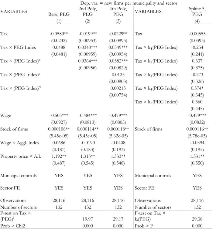
Table 1.2 - Poisson base, polynomial and spline regressions with interactions Dep. var. = new firms per municipality and sector
VARIABLES Base, PEG 2nd Poly, PEG 4th Poly, PEG VARIABLES Spline 5, PEG
(1) (2) (3) (4)
Tax -0.0583** -0.0199** -0.0229** Tax -0.00555
(0.0232) (0.00953) (0.00995) (0.0393) Tax × PEG Index 0.0488 0.0340*** 0.0349*** Tax × k₁(PEG Index) -0.254
(0.0481) (0.00959) (0.00954) (0.241) Tax × (PEG Index)² 0.0364*** 0.0382*** Tax × k₂(PEG Index) 0.337
(0.00956) (0.00829) (0.375)
Tax × (PEG Index)³ 0.0125 Tax × k₃(PEG Index) -0.273
(0.00903) (0.326)
Tax × (PEG Index)⁴ 0.00215 Tax × k₄(PEG Index) 0.574*
(0.00754) (0.345)
Tax × k₅(PEG Index) 0.360
(0.445)
Wage -0.505*** -0.484*** -0.479*** -0.479***
(0.0927) (0.0813) (0.0805) (0.0832) Stock of firms 0.000108** 0.000114** 0.000118** Stock of firms 0.000116**
(5.45e-05) (5.45e-05) (5.62e-05) (5.78e-05) Wage × Aggl. Index 0.0686 -0.0190 -0.0408 -0.0394
(0.181) (0.183) (0.193) (0.195)
Property price × A.I. 1.192** 1.315** 1.333** 1.331**
(0.487) (0.545) (0.548) (0.550)
Municipal controls YES YES YES Municipal controls YES
Sector FE YES YES YES Sector FE YES
Observations 28,116 28,116 28,116 Observations 28,116 Number of sectors 132 132 132 Number of sectors 132 F-test on Tax ×
(PEG)ⁱ 19.97 29.17 F-test on Tax × kᵢ(PEG) 29.38
Prob > Chi2 0.000 0.000 Prob > F 0.000
22 The higher order positive coefficients imply that the deterrence effect of taxes is reduced, at an increasing rate, with a higher level of agglomeration. This is illustrated in
Figure 1.5, using the specification with the 4th order polynomial14.
We can observe that the effect of taxes on firm location is essentially flat and (significantly) negative up to around the 60th-percentile of the distribution. Shortly after the median of the distribution (point 0.5 of the PEG) there is an inflection point in the
14 We estimated 2nd, 3rd and 4th degree polynomial specification. The qualitative results is the same for the
three specification; we show the result for the 4th degree because it is the most visually clear one.
-. 1 -. 05 0 .05 T a x e ff e ct w it h Po isso n 0 .2 .4 .6 .8 1 PEG
Figure 1.4 - Poisson baseline specification
-. 1 0 .1 .2 .3 T a x e ff e ct w it h Po isso n 0 .2 .4 .6 .8 1 PEG
23 slope of the tax effect. This implies that, for the fifth quintile of the distribution of agglomeration, taxes essentially do not play a role for firm location. Indeed, for the most agglomerated sector, taxes have a positive effect on firm location.
Finally, in column 4 of Table 1.2 we present spline regressions, including five splines
over each quintile of the PEG-distribution15. Note that, individually, only the spline term
over the fourth quintile is significant and positive. However, jointly all the terms are highly significant (see F-test at the bottom of the column). The spline regression implies a relatively flat and negative effect of taxes, with an inflection point in the relationship for the fourth quintile and an essentially zero effect of taxes for the most agglomerated sectors.
1.5.2 Percentile regressions with sector fixed effects
We next allow for structural breaks in the relationship between taxes and sectoral agglomeration, using quintile and decile regressions. The results are presented in Table 1.3.
Column 1 shows the regression using quintiles over the agglomeration index (PEG). We can observe that, as before, the main effect of taxes is negative and significant. Interestingly, the only interaction term individually significant (and positive) is the one for the fifth quintile. Results are similar when estimating the interaction terms over deciles, in
which case only the ninth and tenth percentile terms are significant.16
Figure 1.6 illustrates these results for the quintile regression. Note that the tax effect is essentially flat and negative over the first four quintiles of the PEG-distribution. One can detect a slight inflection in the tax effect for the fourth quintile, but the jump is not significant. However, the tax effect is starkly different for the most agglomerated sectors, where it actually turns positive.
15 The results using ten spline terms are qualitatively similar and available upon request. 16 However, the main effect is, albeit negative, not significant anymore.
24 Table 1.3 - Poisson percentile regressions with interactions
Dep. var. = new firms per municipality and sector
VARIABLES Quintiles of PEG VARIABLES Deciles of PEG
(1) (2)
Tax rate -0.0474* Tax rate -0.0695
(0.0288) (0.0540)
Tax × Aggl. Index × q₁(PEG) 0.0850 Tax × Aggl. Index × d₁(PEG) 0.653
(0.117) (0.647)
Tax × Aggl. Index × q₂(PEG) -0.0145 Tax × Aggl. Index × d₂(PEG) 0.207
(0.101) (0.239)
Tax × Aggl. Index × q₃(PEG) -0.0381 Tax × Aggl. Index × d₃(PEG) 0.0740
(0.0512) (0.214)
Tax × Aggl. Index × q₄(PEG) 0.0307 Tax × Aggl. Index × d₄(PEG) 0.0679
(0.0483) (0.166)
Tax × Aggl. Index × q₅(PEG) 0.154*** Tax × Aggl. Index × d₅(PEG) 0.0605
(0.0444) (0.112)
Tax × Aggl. Index × d₆(PEG) -0.00373
(0.0950)
Tax × Aggl. Index × d₇(PEG) 0.0380
(0.0849)
Tax × Aggl. Index × d₈(PEG) 0.0725
(0.0786)
Tax × Aggl. Index × d₉(PEG) 0.146**
(0.0614)
Tax × Aggl. Index × d₁₀(PEG) 0.191***
(0.0654)
Wage -0.486*** Wage -0.477***
(0.0830) (0.0845)
Stock of firms 0.000120** Stock of firms 0.000125**
(5.65e-05) (5.83e-05)
Wage × Aggl. Index -0.0198 Wage × Aggl. Index -0.0430
(0.195) (0.195)
Property price × A.I. 1.313** Property price × A.I. 1.323**
(0.544) (0.545)
Municipal controls YES Municipal controls YES
Sector FE YES Sector FE YES
Observations 28,116 Observations 28,116
Number of sector 132 Number of sectors 132
F-test on Tax × PEG × qᵢ(PEG) 23.22 F-test on Tax × PEG × dᵢ(PEG) 67.61
Prob > Chi2 0.000 Prob > Chi2 0.000
25
1.5.3 Regressions with sector and municipal fixed effects
When estimating equations (28), (30) e (32) including sector and municipal fixed effects we do not obtain the main effect of taxes anymore. Table 1.4 presents these results applying the same specifications as before, i.e. polynomial, spline and percentiles, while Figure 1.7 illustrates them.
The results are consistent with the ones presented above. In column (2) and (3) we present 2nd and 4th order polynomials. Note that the linear and squared terms are highly positive and significant in both specifications. In the 4th order polynomial, all terms are jointly significant (see F-test at bottom of the column).
Similarly, the five-step spline results in only the fourth spline term to be positive and significant, again as in the specification without municipal fixed effects. Finally, using quintiles of the agglomeration index, we obtain anew that the interaction for the fourth and fifth quintiles are positive and statistically significant.
Overall, these results confirm our findings from above. A relatively flat effect of taxes for a large range of sectoral agglomeration, with a strong and positive interaction term for the most agglomerated sectors.
-. 1 0 .1 .2 T a x e ff e ct w it h Po isso n 0 .2 .4 .6 .8 1 PEG
26 Tab le 1. 4 - P ois so n po lyn om ial, sp lin e, a nd quin tile re gr es sio ns w ith se ct or a nd m un icip al f ix ed e ff ec ts w ith no in te ra ct io ns D ep . v ar . = n ew fi rm s p er m un ici pa lit y a nd se ct or V A RIA BL E S 2n d P oly , PEG 4t h P oly , PEG V A RIA BL E S Sp lin e 5 , PEG V A RIA BL E S Q uin tile s o f PEG (1 ) (2 ) (3 ) (4 ) Tax × P EG In dex 0. 01 69 ** 0. 01 93 ** * Tax × k ₁ (P E G I nd ex ) -0 .3 12 Ta x × A. I. × q ₁ (P E G) 0. 18 9 (0 .0 06 61 ) (0 .0 06 40 ) (0 .2 39 ) (0 .1 64 ) Tax × ( PEG In dex )² 0. 02 65 ** * 0. 02 62 ** * Tax × k ₂ (P E G I nd ex ) 0. 48 2 Ta x × A. I. × q ₂ (P E G) 0. 03 53 (0 .0 07 63 ) (0 .0 06 50 ) (0 .3 69 ) (0 .0 99 0) Tax × ( PEG In dex )³ 0. 00 43 7 Tax × k ₃ (P E G I nd ex ) -0 .5 17 * Ta x × A. I. × q ₃ (P E G) -0 .0 27 1 (0 .0 07 88 ) (0 .3 06 ) (0 .0 59 3) Tax × ( PEG In dex ) ⁴ -0 .0 02 51 Tax × k ₄ (P E G I nd ex ) 0. 86 6* * Tax × A. I. × q ₄ (P E G) 0. 04 27 (0 .0 07 98 ) (0 .3 47 ) (0 .0 47 8) Tax × k ₅ (P E G I nd ex ) -0 .3 06 Ta x × A. I. × q ₅ (P E G) 0. 09 84 ** * (0 .3 75 ) (0 .0 31 7) Wa ge 0. 01 21 0. 00 88 8 Wa ge 0. 01 33 Wa ge 0. 01 14 (0 .0 95 0) (0 .0 94 8) (0 .0 95 8) (0 .0 95 2) St oc k o f f irm s 0. 00 01 96 ** 0. 00 02 00 ** St oc k o f f irm s 0. 00 01 98 ** St oc k o f f irm s 0. 00 02 05 ** (9 .0 3e -0 5) (9 .4 0e -0 5) (9 .6 7e -0 5) (9 .6 0e -0 5) O bs er va tions 28 ,1 16 28 ,1 16 O bs er va tions 28 ,1 16 O bs er va tions 28 ,1 16 Nu mbe r of se ctor 13 2 13 2 Nu mbe r of se ctor 13 2 Nu mbe r of se ctor 13 2 F-te st on Tax × (P EG ) ⁱ 27 .4 5 38 .5 0 F-te st o n Ta x × k ᵢ (P EG ) 49 .3 9 F-te st o n Ta x × A. I. × q ᵢ (P EG ) 50 .0 2 Pr ob > C hi 2 0. 00 00 0. 00 00 Pr ob > F 0. 00 00 Pr ob > C hi 2 0. 00 00 Robu st sta nd ar d e rr or s i n pa re nthe se s. ** * p < 0. 01 , * * p< 0. 05 , * p < 0. 1
27
1.6 Discussion of results
What do our results imply? One possible interpretation of our results above is that taxes have a deterrent effect on firm location for a large range of sectoral agglomeration (up to the fourth quintile), but that tax